Guest Post by Willis Eschenbach.
I must confess, I use WUWT as a lab notebook on steroids. It reflects my latest work, my latest calculations, my latest graphics, my latest theories. My thanks to all participants who make this possible: Anthony Watts, Charles The Moderator, anonymous moderators around the planet, as well as all the commentators and lurkers who keep me from going off the rails and suggest new avenues to explore. What a time to be alive!
Onwards. Here’s my latest.
I was watching a National Geographic documentary about the use of airborne lidar to look straight down and see through the trees of the Guatemalan jungle to expose Mayan ruins. The commenter said “If we see straight lines on the ground, it’s not natural. It’s something made by man.”
And it’s true—in general, nature doesn’t do straight lines. As the poet said:
“Glory be to God for dappled things –
For skies of couple-colour as a brinded cow;
For rose-moles all in stipple upon trout that swim;
Fresh-firecoal chestnut-falls; finches’ wings;”
I’m reminded of this by what I see as a ludicrous claim—that regarding the climate, one of the more complex systems we’ve ever tried to analyze and understand, mainstream climate scientists say that there is a straight-line linear relationship between changes in the radiation balance at the top of the atmosphere and the surface temperature. This is a central belief in their understanding of the climate:
∆T = λ * ∆F (Equation 1 And Only)
This says that the change (delta, “∆“) in global average surface temperature (“T“) is equal to the change (∆) in “forcing” (“F“) times a constant called lambda (“λ“) that is known as the “equilibrium climate sensitivity” (ECS).
And what is forcing when it’s at home? Forcing is a term of art in climate science. Radiative forcing is defined by the Intergovernmental Panel on Climate Change (IPCC) as:
“The change in the net, downward minus upward, radiative flux (expressed in W/m²) due to a change in an external driver of climate change, such as a change in the concentration of carbon dioxide (CO₂), the concentration of volcanic aerosols, or the output of the Sun.”
The “downward” radiation at the top of the atmosphere (TOA) is the incoming sunshine. It’s all the radiation entering the system.
The “upward” radiation is the longwave thermal radiation heading to space. It’s the total of all the energy leaving the system.
Now, that claim of linearity makes absolutely no sense to me. Let me explain why.
First, the surface temperature can change without affecting the TOA radiation balance. The climate system is a giant heat engine. Heat comes in at the hot end of any heat engine: in this case it’s the tropics. Then it does work with some of the heat, and the rest of the heat is exhausted at the cold end of the heat engine: in this case, the poles.
Note that only part of this heat is converted into work. The rest is just passing through, carried by the ocean and the atmosphere from the tropics to the poles and back out to space. Any variation in the percentage of the total flow which is converted to work will change the surface temperature without any change in the TOA radiation balance.
Next, the climate system isn’t free to adopt any configuration. It is ruled by the Constructal Law, and like a river meandering to the sea, it doesn’t move in straight lines. Like all flow systems far from equilibrium, the river is maximizing flow, and thus the river picks the longest possible path to the sea.
Similaryly, as a constructally ruled system, the climate is always seeking to maximize the flow from the tropics to the poles. And as that flow speed changes, the surface temperature changes … without any corresponding linear change in the TOA radiation balance.
Finally, their Equation 1 equates a quantity that IS conserved (watts per square meter) with a quantity which is NOT conserved (temperature). I’m not clear how that is even possible.
However, for the purpose of this discussion, let’s assume that they are right about that particular relationship between TOA forcing and temperature. We’ll follow that path and see where it leads.
As a first step along that path, let me return to the idea that the climate doesn’t move in straight lines. For example, below is a graph of gridcell-by-gridcell total cloud cooling/warming, which is a combination of the clouds’ effects on longwave and shortwave radiation plus the evaporative cooling related to rainfall. I’ve compared it to gridcell surface temperatures in a scatterplot with contour lines.
Now, I started doing these scatterplots like in Figure 1 below, comparing two variables for every 1° latitude by 1° longitude gridcell of the planet, for a simple reason. They show the long-term relationship between the two variables. Each gridcell on the planet is in a long-term, general steady state regarding the various measurable factors, like say thunderstorm prevalence. Annual averages of these relationships vary little, and a 24-year average reveals the underlying long-term relationship of the variables.
And this lets us investigate things like the long-term value of the equilibrium climate sensitivity … but I get ahead of myself …

Figure 1. Scatterplot plus density contour lines and LOWESS smooth. Total cloud cooling versus surface temperature, entire planet.
Back to figure 1, there’s much of interest. First, in gridcells with average temperatures below about -20°C, which is Greenland and Antarctica, the clouds warm the surface. Then when the frozen ocean comes into play, from -20°C to where the gridcells average about freezing, there is cooling increasing with temperature.
Then the trend reverses, and cooling decreases with temperature up to the gridcells with an average temperature of 25°C or so. And above that, the cooling increases radically and almost vertically to the point where it is cooling those gridcells by -400 W/m2 or so.
In passing, note the peak around 25°C. If the temperature goes above that, the clouds increase their cooling, eventually to a radical extent. And when the temperature goes below ~ 25°C, the clouds decrease the amount of cooling. This is clear evidence of the thermoregulatory action of clouds, cooling more when it’s warmer and less when it’s cooler.
Finally, the predominant role of the ocean is evident in both the tighter grouping and the larger number of the blue oceanic dots compared to the brown dots showing land gridcells.
And to close the circle, the red/black line showing the change of cooling with temperature is kinda the definition of non-linear …
Now, these kinds of graphs are very useful for a simple reason. The slope of the red/black line at any point gives the average change in the y-axis variable for a 1°C change in the surface temperature. So for example, we can see that when it’s above say 25°C, the total cloud cooling increases extremely rapidly with each 1°C increase in temperature.
With all of that in mind, what can such graphs show us about the long-term relationship between temperature and forcing?
The mainstream theory goes like this:
- Doubling the amount of CO2 intercepts more of the upwelling longwave radiation headed to space.
- This leads to a top-of-atmosphere (TOA) radiative imbalance.
- The Earth then warms up until the balance is restored.
So the question becomes … how much does the earth have to warm up to restore the 3.7 watts per square meter (W/m2) of TOA radiation imbalance that is said to result from a doubling of CO2 (2xCO2)?
This amount of warming required to rebalance the TOA radiation imbalance is called the “equilibrium climate sensitivity” (ECS) to a doubling of CO2. It’s the “lambda” in the linear Equation 1 (and only) above.
To investigate the value of the ECS, here is the scatterplot of the TOA imbalance versus the surface temperature.

Figure 2. Scatterplot plus density contour lines and LOWESS smooth. Top of atmosphere radiative imbalance versus surface temperature, entire planet. The percentage (% area) numbers show the percentage of the surface area in each temperature interval.
Man, I love being surprised by my investigations. It’s the best part of my scientific education. I definitely did not expect the graph to look like that. But facts are facts.
At temperatures below -20°C, the brown dots show it’s just land— Greenland and Antarctica. And there, curiously, the TOA imbalance gets more negative for each 1°C of warming. Then, at around -15°C, the slope reverses as the frozen ocean comes into play. It increases, somewhat linearly, until about 20°C or so, after which the imbalance starts increasing at a faster rate.
We can visualize these changes in detail by calculating the slope at each point in the red/black line. Recall that the slope is the change in TOA radiation imbalance per degree of warming. Here is that result.

Figure 3. Slope of the red/black trend line shown in Figure 2 above. If you wonder why the area-averaged change is so high, look at the percentages of the global area with annual average temperatures in each temperature interval.
I’ve included the area-weighted average of the change in the TOA balance from a 1° increase in surface temperature. It’s 6.6 W/m2 per °C. This implies an equilibrium sensitivity (ECS) of 0.6°C per doubling of CO2
I’m gonna say that is a reasonable estimate for the ECS, for a couple of reasons.
First, this ECS estimate of 0.6°C is not outside the range of other observational estimates of CO2 sensitivity. In the Knutti dataset there are the results of 172 people’s calculations of the ECS, using different methods. My estimate is at the low end, but it isn’t the lowest.

Figure 5. Estimates of ECS from theory and reviews, observations, paleoclimate studies, climatology, and climate models. Note that in the last half century these estimates have grown more scattered, not less. And it’s particularly true for climate models (yellow dots).
The second reason I think that my ECS estimate of 0.6°C per 2xCO2 is valid is that it agrees with what I said about my previous estimate of the ECS, which was based on my implementation of Bejan’s Constructal climate model. The model is described in the post below.
I fear most folks don’t understand the importance of the model of the global climate system that Bejan created. As I showed, it does a very accurate job of calculating several critical parameters of the climate using one and only one tuned parameter, the conductance. Conductance in this context is how fast the climate system can move the heat from the hot zone to the cold zone. The agreement of the model with reality is shockingly good. Read the post.
Using that model, I was able to experimentally determine my best estimate of the climate sensitivity. From that previous analysis:
This constructal model points out some interesting things about climate sensitivity.
First, sensitivity is a function of changes in rho (albedo) and gamma (greenhouse fraction). But not a direct function. It is the result of physical processes that maximize “q” [the flow from the hot zone to the cold zone] given the constraints of rho and gamma.
Next, the sensitivity is slightly different depending on whether the changes in albedo and greenhouse fraction are occurring in the hot zone, the cold zone, or both.
Next, assuming that there is a uniform pole-to-pole increase of 3.7 W/m2 in downwelling radiation from changes in either albedo or greenhouse fraction, the constructal model shows a temperature increase of ~1.1°C. (3.7 W/m2 is the amount of radiation increase predicted to occur from a doubling of CO2.)
Finally, this 1.1°C equilibrium climate sensitivity is a maximum sensitivity which does not include the various emergent thermoregulatory mechanisms that tend to oppose any heating or cooling. This means the actual sensitivity is lower than ~1.1°C per 2xCO2.
And my latest estimate, 0.6°C per 2xCO2, is indeed lower than the upper bound of 1.1°C per 2xCO2 found in Bejan’s model, just as I’d predicted.
And thus endeth my disquisition about non-linearity and how it led me to my latest ECS estimate.
My warmest regards to everyone, as always.
w.
PS—When you comment, please quote the exact words you are referring to. I choose my words carefully so I can defend them. I cannot defend your restatement of my words, no matter how well-meaning.
Funny how calculations of ECS with observations are always lower than model estimates!
Regarding figure 2, people can forget that the poles in winter are major emitters of radiation. No sun to melt ice and thus absorb energy, freezing melt water from the summer sends radiation to space, and the total lack of clouds allows more radiation to go to space. Finally, more meridional energy transport to the poles is accomplished because winters are stormier than summers, and mid-latitude storms transport most of the tropical heat to the poles.
Good post Willis, very interesting.
Andy May, there is one exception. It is INM CM5 in CMIP6. It produces an ECS of 1.8, which is within the observational uncertainty of EBM estimates. I tend to rely on the second Lewis and Curry paper (LC18, available at Climate Etc), which addressed a number of criticisms to their first (LC15). The 2 sigma ECS uncertainty range of LC18 is 1.2C-1.95C.
The reason I find this important is that INM CM5 is the only model in CMIP6 that does NOT produce a spurious tropical troposphere hotspot. So important the Russians published a whole paper on why—they simply parameterized ocean rainfall using actual ARGO observations. About twice the ocean rain, about half the water vapor feedback, so about half the ECS of the CMIP6 median.
A side ECS observation. Whether WE is ‘right’ here, supported by Bejan’s Constructal model, or LC18 and INM CM5 are ‘right’ isn’t as important as the bigger conclusion that either way the ‘climate alarm’ should be cancelled.
Thanks, Rud. Indeed, the climate alarm should be put in the dustbin of history. We have real problems and challenges on this benighted planet, but that ain’t one of them …
w.
WE, it eventually will be. But I fear dustbinning will be a slow process.
Like all manias, it will eventually end. I think we are closer to that end now that alarming projections of the past have proven false, and the enormous problems with renewables and ‘electrification’ are becoming obvious.
Sadly true, my friend. As Upton Sinclair remarked,
w.
Willis –
or was it Ambrose Bierce?
Further research proves you to be right, Willis. My apologies for doubting you.
No need for apologies, atticman. Doubt is an essential characteristic for a scientist.
w.
— Jonathan Swift
Another good one! And funny how all of these parcels of well expressed wisdom apply so perfectly to the climate delusions.
Hi Rud, Just one comment. IMHO, both Lewis and Curry and INMCM5 make the critical assumption that all warming outside their assumptions (for L&C the AMO and INMCM5, deep ocean layer) is due to CO2. Now, I believe in the deep ocean layer and in the influence of the AMO, I just don’t like the assumption that 100% of the warming outside of those factors is due to CO2.
As a result, I consider both L&C and INMCM5 to be the highest possible values of ECS. I think the true value is less and WE’s estimate is very reasonable, but who knows? I’ve been wrong before.
AM, agree with your assumptions critique of LC18. Disagree with your conclusions.
I have calculated several different independent ways (Lindzen Bode feedback from his 2011 paper, Monckton’s ‘Irreducibly Simple’ 2016 paper, a number of non EBM estimates like Callendar 1936) that the most probable ECS lies somewhere between 1.5 and 1.8. Well within the central EBM uncertainty range.
Separate underlying logic check comparing just feedbacks/no feedbacks.
Curry at Climate Etc (~2010 no feedbacks ECS ~1.1) and Lindzen 2011 (no feedbacks ~1.2), and Monckton’s 2016 (no feedbacks 1.16), plus we know from Dessler 2010b that observational cloud feedback is roughly zero (confirmed by McIntyre redoing Dessler in 2011), plus from IPCC AR4 and AR5 that the sum of all other feedbacks excluding water vapor feedback is also about zero, plus from Clausius Clapeyron that water vapor feedback must be something positive, then the ‘true’ ECS must be something greater than 1.2.
NOT almost half of 1.1 as figured here.
Given that either result cancels climate alarm, I decided not to spend any further energy parsing the ECS difference between my several and WE’s several estimates.
Perhaps you are correct, but all your calculations assume net feedback is >= 0. It isn’t hard to imagine net feedback is < 0, after all that is normal in nature.
Either way, we should be able to agree ECS < 2 and > 0 and that AR6 is too high.
Thanks, Rud, I agree that either result cancels climate alarm.
However, I disagree about the Planck no-feedback parameter. You calculate it using a temperature of 255K.
255K is the temperature of an imaginary superconducting blackbody planet receiving ~ 240 W/m2 from the sun, the same amount of radiation that the Earth’s climate system receives.
In another thread,I asked why use 255K, but you might not have seen my question.
Using 255K as a temperature, the no-feedback sensitivity is (3.7 W/m2 per 2x CO2) / (4 * sigma * 255^3), where sigma is the S/B constant, 5.67e-8. This is 1.0°C per doubling of CO2 as you say.
HOWEVER, the planet is not at 255K. It’s at about 288K. This makes the current real-world no-feedback sensitivity (3.7 W/m2 per 2x CO2) / (4 * sigma * 288^3). This is 0.7°C per doubling of CO2.
Why use a blackbody temperature of an imaginary superconducting blackbody planet when we have current real-world temperature to calculate a current real-world no-feedback response?
w.
Excellent point.
Late on a mostly dead thread, for archival purposes.
I went and looked up Judith’s post on zero feedback sensitivity from 11 Dec 2010. The 255K is the temperature at the effective radiating level (ERL), not the 288K surface. Seems logically correct to me.
But, in support of this general post, she also concluded by saying there are still many in certainties, and that delta T= lambda delta F is NOT written in stone.
Not late at all. But I don’t see the logic. We’re not talking about GHGs changing the temperature of the ERL. Equation 1 (and only) doesn’t refer to the ERL. It is talking about the change in surface temperature, not the ERL temperature.
The ERL is an imaginary level of the atmosphere where the temperature is high enough to radiate 240 W/m2, to match the solar input. That’s where the temperature is 255K (-18°C).
But that’s imaginary. In fact, what’s increasing in temperature if GHGs increase is the surface due to increased downwelling radiation. This increases outgoing radiation, and the surface temp keeps going up until once again the outgoing radiation increases to match solar input.
And at that point, the ERL is … right back to where we started.
Any clarification welcome.
w.
Here’s calcs of 2xCO2 using UChicago Modtran. Humidity varying with Temp (fixed RH), clear sky tropical conditions….TOA heat in=IR out…. Gives 1.21 C per doubling. Mid-latitude winter gives 0.82 C per doubling. So presumably averaged over the planet, about 1C per 2xCO2. I am open to anyone’s logic as to why Modtran would be so drastically wrong…but “observations” on WE’s fig 5 say 2.7….I would challenge the sources of this, the lab measurements of IR absorption used in Modtran are “observations” as well…and actual observations of energy in the atmosphere are quite difficult, changing cloud cover, changing water vapor with altitude that needs a radiosonde to decipher unless you make some parameterized assumptions about your satellite sensors.
WE….your Fig. 3 …..ECS 0.6 C per doubling….very impressive how you snuck that into the fine print……we’ll see if you get taken to task by anyone on that…gotta say I love those area annotations on your graphs….and the LOWESS fits….makes the plot so much more meaningful….
Thanks, D. I am always searching for ways to pack more info into a single graphic. This time around, I’ve added the contour lines, making the differences more visible, and the area annotations.
w.
‘I am open to anyone’s logic as to why Modtran would be so drastically wrong…’
Here’s mine:
Notwithstanding very large variations of atmospheric CO2, a ‘radiative forcing’ over geological time, there’s absolutely no evidence that these variations have had any impact on the Earth’s temperature.
Given the above, it’s fair to conclude that ‘radiative transfer models, like MODTRAN, universally miss the boat on how the energy of thermal radiation that is absorbed by IR-active gases within meters of the surface is conveyed through the troposphere and eventually emitted to space.
Thanks Frank….what I am getting at here is that UChicago Modtran results in lower ECS than the GCM’s. And “conveyance through the atmosphere” must be convection and advection to polar regions…which one would think would result in a lower ECS than the clear sky multi-layer radiative approach of the Modtran numbers. But you can enter cloud cover and rainfall scenarios into Modtran, so obviously a number of non-radiative parameters must be included in the UChicago “simulations”. But they are pretty accurate judging by their examples….so the issue remains unanswered, why is ECS 1.21 by UChicago Modtran but higher on most of the Fig.7 points that WE has plotted ? Anyone got an inkling to add to Frank’s?
DM, there’s the old adage that ‘if you’re a hammer, everything looks like a nail’. Both MODTRAN and the ‘GCMs’ suffer from the ‘core’ assumption that radiative transfer aptly describes the role of GHGs in the troposphere. Furthermore, the GCMs suffer from additional ‘parameterized’ assumptions, e.g., positive water vapor feedbacks, that would explain why the projections of the models are vastly higher than those provided by MODTRAN and those obtained ‘independently’ by many climate alarm skeptics.
The problem is that none of the above results are truly independent, since all of them ignore how the behavior of IR-active gases is vastly changed by collisions with the non-IR active gas species that comprise the vast bulk of the atmosphere, as well as conflating the radiative properties of condensed matter and gases.
The figures will be about 1/3 lower once you introduce clouds to the model. The modtran options seem very restricted, but it works nonetheless, if you know what you are doing.
However, modtran does not change the lapse rate. With warming you a get a smaller lapse rate, and that is a huge negative feedback. Like this..
https://greenhousedefect.com/the-holy-grail-of-ecs/the-climate-kill-switch-why-feedbacks-are-actually-negative
Thanks ES….I also get significant reduction with clouds….By saying things like “worst case clear-sky equatorial”, I hope to encourage border-liners to try UChicago Modtran themselves so they can form their own CC/Radiatve/CO2 opinions and self-learn sufficient info to counter in a science based way…the idiotic opinions they will be forced to listen to….on both extremes of the debate…(range of GHE-doesn’t-exist to waste-heat-will-boil-the-oceans-in-400-years-Sabine-Hossenfelder)
“Forcing is a term of art in climate science.” You’re much too generous 🙂
Another great diminution of CO2’s impact on Climate. Thanks Willis.
“The “downward” radiation at the top of the atmosphere (TOA) is the incoming sunshine. It’s all the radiation entering the system.”
Don’t forget non-sunshine related energy coming in. Energetic particles (protons, cosmic rays and the like) as well as all that energy coming from solar flares and coronal holes. Not only does it introduce energy, it also changes the electric circuits between the earth and space. Weather systems strengthen, earthquakes happen, winds change, dogs and cats living together.
With the weakening of the Earth’s magnetic field over the past couple of decades, the impact is picking up.
Thanks, r. While these may or may not affect the climate, the energetic amount is tiny. I find the following, below.
w.
PS: As to sunspots and their associated changes in heliomagnetism and thus cosmic rays affecting earthquakes, see my post below.
https://wattsupwiththat.com/2020/01/25/spot-the-quakes/
===
Energy Input to Earth from Energetic Particles and Solar Activity
Overview
The energy added to Earth from energetic particles—such as protons, galactic cosmic rays, and solar energetic particles—as well as from solar flares and coronal holes, is a small but important component of the total energy budget received by our planet. This is distinct from the much larger energy input from solar electromagnetic radiation (the solar constant, ~1361 W/m²) [1] [2].
Typical Energy Fluxes (W/m²)
| Source | Approximate Energy Flux (W/m²) | Notes |
|Solar wind (average) | 0.03–0.06 | Continuous, includes protons and alpha particles [3]
|Galactic cosmic rays | ~0.00001 | Very small, steady background [4]
|Solar energetic particles | ~0.0001 (during events) | Highly variable, short-lived bursts [5] [6]
|Coronal hole high-speed wind| ~0.01 | Variable, associated with coronal hole streams [7]
• Total average energetic particle energy flux: ~0.05 W/m² (sum of all above sources)
[1] https://www.e-education.psu.edu/eme812/node/644
[2] https://en.wikipedia.org/wiki/Solar_irradiance
[3] http://arxiv.org/pdf/2101.03121.pdf
[4] https://sites.astro.caltech.edu/~srk/MiniCourse/Stefano_Gabici_CR.pdf
[5] https://www.aanda.org/articles/aa/full_html/2023/02/aa45810-22/aa45810-22.html
[6] https://www.ntanet.net/solar-flares-impact-on-astronauts-and-earth/
[7] https://www.aanda.org/articles/aa/full_html/2022/03/aa41919-21/aa41919-21.html
[8] https://www.sciencedirect.com/science/article/pii/S0273117721008814
Willis,
Indeed, the total of energy from incoming miscellaneous energetic particles looks to be a bit less than outgoing radiation from geothermal sources. Wikipedia puts the outgoing at 0.0916 w/m**2 and cites Donald L. Turcotte; Gerald Schubert (25 March 2002). Geodynamics. Cambridge University Press. ISBN 978-0-521-66624-4.
This is an interesting hypothesis. Most of the energy from cosmic rays and the like is deflected to the magnetic poles for making aurorae and general tidiness.
What would be the impact of increased cloud seeding away from the poles?
No one would say that, because there is no “downwelling longwave radiation” at the top of the atmosphere. Where would that come from? Mars??
Thanks, E., good catch. I’ve changed it as follows:
Best regards,
w.
Wait a minute! The sun doesn’t radiate long-wave radiation? It may not be large in terms of heat transfer compared to short wave but it *does* exist.
‘The sun doesn’t radiate long-wave radiation?’
As a ‘black body’ it emits EMR at all frequencies, but only in negligible amounts at the long-wave frequencies relevant to Earth’s emissions of same.
Those curves are not black body emission curves. Abut 48% of sunlight is IR light with 37% near and mid IR light and 11% far IR light (0-5000 wavenumbers).
The warmth of sunlight is mostly due to the near and mid IR light.
Sounds about right. I’ve not done the integrals, but the curve of sunlight intensity vs wavelength shows a peak in the visible spectrum (reasonable, since that’s what our eyes are meant to see) with a long tail beyond red.
Incidentally, satellite photos of the daytime Earth show considerably brighter color radiation than nighttime. In addition to the reflection from the white clouds, I’m not sure that the pretty blues, greens, and browns should be ignored.
And the Earth is ( of course) NOT a blackbody, making the equations at least problematic.
Furthermore, radiative ‘forcing’ or impact ( absorbtion, emission and interaction) is also not as straightforward as often assumed given the different vibrational modes of various amounts of molecules. I still see all this as a guessing game..
The average emissivity of the earth is 0.98, so treating it as a blackbody only introduces a tiny error.
w.
Those curves certainly are black body emission curves, here’s the linear version of the Sun, showing the proportion of IR:
http://hyperphysics.phy-astr.gsu.edu/hbase/imgmod/wien.gif
Willis, how did you first calculate the TOA radiation imbalance (versus Temperature) for Figure 2?
While I applaud your efforts, the link to CO2 is suspect. It can be shown T2m is strongly correlated to SST with a one month lag, and that SST is not affected by CO2, but rather the opposite.
The assumed 2xCO2 forcing should produce a growing trend in T2m vs SST, but the difference in these two trends after 65 years is so small as to imply actual 2xCO2 forcing is negligible or zero.
The imbalance figures are from the CERES satellite dataset entitled “toa_net_all”.
w.
Thanks. Personally I prefer “net” to “imbalance”. Quoting you from 10 years ago:
I honestly thought you might have calculated it yourself Willis, just for the heck of it.
Even though I use the CERES EBAF it’s still odd to me when net is called an imbalance.
Asfaik we don’t refer to any other net quantity in climate science as an imbalance.
The use of imbalance implies there was a time when it was in balance. Was it ever?
From the AGU, Earth’s Energy Imbalance More Than Doubled in Recent Decades
In order to believe the Earth is out of balance according to this paper’s authors, one must believe in AGW wholeheartedly, that emissions are the reason for the so-called imbalance.
The entire idea of climate energy accumulation starts with the sun, clouds, and the ocean. Everything else in the climate follows, including the atmosphere. So as much as I admire these authors and their data collecting abilities, I am at odds with their AGW beliefs.
No and no!
What the IPCC means are the “fluxes” at the tropopause! If you have an increase in CO2 for instance, you will get an increase in “downwelling radiation” from the stratosphere, and a decrease in “upwelling radiation”. For instance like 1.3 – (-2.4) = 3.7W/m2.
That is why the IPCC definition continues like this..
That is because the change in the temperature of the stratosphere affects the “downward flux” at the tropopause. I have explained this many times over. You should really start reading my stuff, which is light years ahead..
https://greenhousedefect.com/unboxing-the-black-box
Thanks, E., but that’s a direct quote from the IPCC. The IPCC also says (emphasis mine):
You’re free to redo the analysis with some other definition of forcing. That’s the definition I’m using because it’s the IPCC’s definition, and I wanted to understand where that definition leads.
w.
PS—I’m also using that definition because it can actually be measured. You advocate using “stratospherically adjusted radiative forcing”, which cannot be measured because it is an imaginary construct.
Instead, as you say, “stratospherically adjusted radiative forcing is computed with all tropospheric properties held fixed at their unperturbed values, and after allowing for stratospheric temperatures, if perturbed, to readjust to radiative-dynamical equilibrium.”
In other words, “stratospherically adjusted radiative forcing” is nothing but the output of a computer model for an imaginary situation that has never happened in the real world.
Hard pass.
It is not my definition, but it is what “the science” assumes. Again, Myrrhe, Stordal 1997 explains this pretty well. I can assure you the “downwelling” part from the stratosphere is irrelevant and CO2 forcing thus much smaller.
Also it states they would account for “tropospheric adjustments”, meaning changes in the lapse rate. That’s not true either. What actually happens is the lapse shrinks, because WV, the troposphere warms more than the surface (aka tropospheric hot spot). This increases the upward flux and reduces the CO2 forcing itself.
The relation goes like this. Doubling CO2 will increment CO2 forcing by ~12% (bear in mind the given stock CO2 concentration is also a forcing). With every K in surface warming, the lapse rate shrinks by ~2%, so the GHE and every GH-agent, so that with 6K warming CO2 forcing falls back to its original level, despite having doubled. They do not take this into account, because they can’t.
In fact the combined WV-LR feedback is negative, and they know it. In order to “fix” this a trick is applied:
(AR6. 978)
Their problem is the huge negative LRF, also affecting CO2 forcing. If they’d let physics and logic rule, they end up with a negative feedback all over, and minimal ECS. To fix it they just hard-code a positive WV+LR feedback of plus 1W/m2 into the models.
E., you say “It is not my definition, but it is what “the science” assumes.”
I just gave you the quote from the IPCC saying that THEY assume a TOA measurement, not some imaginary “stratospherically adjusted radiative forcing”.
As I said, you’re free to analyze some fantasy unmeasurable computer model outputs that have NEVER occurred on the real planet. Seriously, there’s nowhere on or above the Earth that you can measure “stratospherically adjusted radiative forcing“.
It is only found in computer model outputs, and without real-world data to compare them to, how do you know if they are even in the imaginary ballpark?
But hey, write it up, send it to Charles The Moderator, and you can discuss it with whoever is interested.
Me … I’m not.
Best to you and yours,
w.
Most “climate scientists” do not know their own science. I know Schmidt et al 2010, or Held, Soden 2000, where they claim CO2 forcing was about the difference it makes TOA. They think doubling CO2 would yield 3.7W/m2 in less outgoing radiation. Of course that is not true.
They do not care, because basically they are just playing their models. And as Rasmus Benestad put it, after “explaining” the GHE he does not understand:
“Computer code used in climate models contain all the details”
It is a “science” they believe in, not something they know about. Given these circumstances, it is not hard to find quotes giving the wrong idea. The hard part is properly understanding this stuff after all..
“I’m also using that definition because it can actually be measured.”
That’s a good criterion to use, Willis. Keep that one in mind.
“cannot be measured because it is an imaginary construct.”
Now does that only apply to other people’s “imaginary constructs”, or does it also apply to your own, such as that downwelling longwave infrared power you keep banging on about? Not to mention every single “flux” in your “steel greenhouse”?
Steve, give it up. No way I’m going to answer your unhinged rants. Go bother someone else.
w.
“Unhinged rants”? I’m just asking you to follow your own advice. How is that “unhinged”? Unless you yourself are “unhinged”, of course.
And naturally we can conclude, as usual, that this claim of yours is simply another damned lie: “I choose my words carefully so I can defend them”
Because you have neither the ability nor the intention to defend any of your hundreds of claims about “radiant flux”, which cannot be measured. According to your own definition, that makes it an imaginary construct. Glad we got that sorted out!
Pass. First Rule Of Pig Wrestling applies, viz:
Have a good life,
w.
[SNIPPED—I told you very clearly that I’m not going to debate with you. You seem to enjoy it and I just get dirty. Go attack someone else.]
Yes, Willis, I do enjoy debating physics. I asked you a simple physics question: why should we consider your numerous claims about unmeasurable “radiant flux” to be anything other than an “imaginary construct”, according to your own definition of that term? Remember, you said you choose your words carefully and can defend them. Was that claim a lie?
Please cease the endless insults and stick to the science. Thanks.
Pass.
w.
No science, then, just lies… as usual…
” if you have an increase in CO2 for instance, you will get an increase in “downwelling radiation” from the stratosphere, and a decrease in “upwelling radiation”.”
bah humbug
A more general related comment concerning Figure 5. ‘Climate science’ is perhaps the only ‘science’ where a crucial value—ECS— becomes less rather than more certain with time. Unsettling. The value of pi, the mass of a proton, the speed of light, ‘g’ the force of gravity, age of the universe all got more certain after more scientific ‘work’.
True Rud. I’ve long held that this increasing uncertaint is prima facie evidence that the underlying model of
∆T = λ * ∆F
is just a convenient fantasy.
w.
In addition, the velocity of gravitational waves and the velocity of light appears differ less than 1 part in 10^15.
Good enough for government work.
Once again a very interesting post; many thanks.
Regarding figure 3: Willis, would it be possibly to present the area-weighted average for land only? Just very curious how much ‘higher’ that figure will be since land warms more rapidly (but subsequently loses more heat via radiation).
Nicely done, Willis! Thank you for this most enlightening post.
Of course this analysis assumes the CERES EBAF values are valid for the purpose used. For generating the highly revealing scatterplots from the gridded data, this seems reasonable.
For the purpose of arriving at an estimated ECS for the 2XCO2 case, it seems important to note the magnitude of adjustment to the observed values to arrive at the TOA EBAF values. This is documented here, which is currently linked at the NASA CERES web page for EBAF 4.2 as a reference. The paper is Loeb, et al 2018, which was published for the EBAF 4.0 version.
https://journals.ametsoc.org/view/journals/clim/31/2/jcli-d-17-0208.1.xml
“Importantly, the SW and LW TOA flux adjustment is a one-time adjustment to the entire record.”
From Table 5, the all-sky adjustments to outgoing LW and SW show a net reduction in the computed imbalance from 4.3 W/m^2 to 0.71 W/m^2 (i.e. constrained by estimated heat storage.) So this adjustment is of the same magnitude as the 2XCO2 no-feedback radiative effect, widely assumed to be 3.7 W/m^2 as you note.
No one, to my knowledge, has yet established at the outset of any modeling or analysis exercise that a 2XCO2 change in atmospheric composition must indeed operate as a “forcing” so as to de-rate the LW emitter.
David,
That Loeb et al paper contains “CERES instrument calibration uncertainty is 1 W m−2 (1σ).”
I seriously doubt that estimate. Much of what Willis wrote here is affected by it.
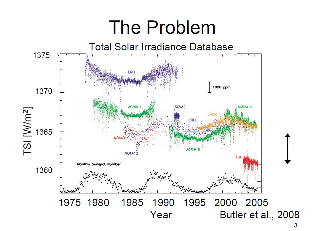
I am past doing it, but it might be interesting to re-do the Willis article using only TSI data from the latest satellite, rather than an aggregation involving earlier one and their huge differences. The downside is a shorter data period. Geoff S
Thanks for this reply, Geoff. Agreed. Yes, the entire narrative of the “earth energy imbalance” pretends that the imbalance comes from measuring LW and SW from space. This is terribly misleading. I do think the CERES LW and SW hourly gridded data (not the EBAF but the unadjusted) is a good way to show the variability and the critical influence of cloud formation and dissipation. But to expect to calculate an imbalance using the same data has been problematic (being generous!) all along.
I have often seen estimates here on WUWT of ±1 – 4 W/m² as a measurement uncertainty figure for these numbers. 4/1360 is a 0.3% uncertainty. That is very good for a field instrument.
“Finally, their Equation 1 equates a quantity that IS conserved (watts per square meter) with a quantity which is NOT conserved (temperature). I’m not clear how that is even possible.”
I might be missing something here. A governing axiom of nature is generally stated as Mass and Energy are conserved. That would be kilograms and Watts. Expressions such as (Equation 1 and only) are encountered throughout engineering of all kinds, and very likely in science, too. They relate a flux/flow to a driving potential.
An example that is universally found and universally accepted in engineering is energy exchange due to temperature differences. qw = hc * ( Tw – Ts ), where, hc is a heat transfer coefficient, Tw is wall temperature and Ts is sink/source temperature. There are hundreds of examples in all kinds of engineering disciplines.
These primarily, almost universally, empirical relationships based on measured experimental data generally arise when the governing physical phenomena and processes are of such small temporal and spatial scale that the local-instantaneous driving potential and associated flux/flow cannot be resolved. In some cases, such as heat transfer under turbulent fluid flow, the foundational formulation of the continuous local-instantaneous governing equations are known only to some degree of approximation.
Importantly, accurate numerical solution of even these approximate formulations at the necessary scales is basically an intractable problem. The real-world spatial gradient of the driving potentials is simply too small to be accurately numerically resolved. That flux/flow is then represented by a representative coefficient, or function, and a simple algebraic representation of the driving potential. The representative coefficient will generally be a function of the transport properties of materials for the specific flux/flow of interest.
The application discussed in the post clearly is not in any way related to micro-scales of time and space. However, the same reasoning as used in engineering is applied. A flux/flow that cannot be spatial and temporally resolved is replaced by a representative coefficient times an algebraic representation of a driving potential. Application to Earth’s climate systems is on a massive average approach simply because the scales and enormous number of physical phenomena and processes is beyond using as a basis for top-down discussions.
Climate science places a lot of creditable on an axiom that Earth’s Climate Systems have in the past, and will again at some unspecified times, operate in a steady-state radiative energy balance. The steady-state seems to mean that a Global Average Surface Temperature over a 30-year period will be roughly the same as the average over the previous 30-year period. The starting period is not yet known. Thus the laser focus on radiative “forcings”. For a top-down massive-average simple look, (Equation 1 and only) is used. The use of Equilibrium in ECS is a misnomer as there will never be Equilibrium in Earth’s Climate Systems.
In the early days, the axiom was usually stated with the proviso/assumption “all other things remain the same” while the radiative balance is changing to a heated-up Earth. Clearly the proviso/assumption is extremely difficult to accept because intuitively it seems that heating up Earth is very likely to change something, and all other things will not remain unchanged at the initial conditions.
Dan, always good to hear from you. See my comment below
https://wattsupwiththat.com/2025/07/12/moving-but-not-in-a-straight-line/#comment-4093035
w.
Déjà vu?
Richard S. Lindzen and Yong-Sang Choi
On the determination of climate feedbacks from ERBE data
GEOPHYSICAL RESEARCH LETTERS, VOL. 36, L16705, 2009
That paper was discredited on methodological grounds by 2011.
I’ll have to go over this a couple of more times to sink in, but as far as clouds go, not all clouds are treated equally. High clouds tend to be ‘warming’ mid and especially low clouds tend the be cooling. However this also depends on the time of year. Winter stratus here in the Plains is usually associated with a relative warmer regime, mainly due to above average low temps. As they say, it’s complex!
Mostly those high clouds are just wispier cirrus type and let more sunlight through during the day than “average” clouds…so it’s really the sunlight that should be declared to be doing the “warming”…but one sees this high-clouds-warming meme so often that it is pedagogical….
Willis,
I continue to hold in high regard those scientists who developed equations such as your Equation 1 And Only as well as the satellites and instruments measuring radiation and more. They provided a seminal basis for advancement. When I was concerned about the work, I would offer an opinion such as the following image from a decade ago, with words that questioned the faith given to adjustments of data.
It seems that many of these seminal authors did not follow up in later times with corrections to their work when it was reasonable that they were wrong. Some have died, some are too old, some lost interest and quit. This failure to correct leads to dominant paradigms that are wrong and that seem to be questioned less as time passes.
There is value in presenting data that challenge the paradigms as you have done with your article. I regard this article as a seriously big deal for those currently involved in the art of climate change. It deserves more attention than has typically been given to past dissent and I hope that you get it. We lack progress in having dissenting work considered. I have no ready answers.
I feel qualified to talk about this “failure to correct” because I am a good example of it. I left my 30 years of geochemistry soon after my last employment and seldom revisited the topic. I have little idea if my team and I made mistakes that should be corrected, plus little idea of the present state of the art of geochemistry.
Thank you for an important article beautifully presented. Geoff S
Nice work Willis.
Atmosphere is like a blanket. How thick is said blanket? How thick has said blanket been in the past? What would happen to the thickness of the said blanket if all of the CO2 contained in calcium carbonate deposits were liberated?
‘- Venus
If all of the CO2 contained in calcium carbonate deposits were liberated, it would be the ground – not the sky – where we find difficulties.
No “runaway greenhouse effect” made Venus’ “climate” what it is, and Earth didn’t go through any “runaway greenhouse effect” with 7,000ppm atmospheric levels in the distant past.
And 4,000ppm couldn’t prevent a full-blown GLACIATION 450mya either.
Unless all of the Earth’s water were to disappear (which would be a bigger problem), CO2 is and always will be a non-factor.
Willis appears to misunderstand his equation 1. He says that Eq. 1 ‘
says that the change (delta, “∆“) in global average surface temperature (“T“) is equal to the change (∆) in “forcing” (“F“) times a constant called lambda (“λ“) that is known as the “equilibrium climate sensitivity” (ECS).”
Now nowhere does equation 1 say that lambda is a constant. Rather it is just the slope of the
curve at that particular point and lambda is in fact defined by Eq. 1. And as a result there is not one value of lambda but actually an infinite number of values, i.e. one for every value of the Earth’s temperature. As an example consider a perfect black body which obeys the Stefan-Boltzmann law. This says that the temperature depends on the 4th power of the incident radiation and as such the ECS would vary from being infinite at zero kelvin to zero at an infinite temperature.
Next Willis goes on to say that:
“Finally, their Equation 1 equates a quantity that IS conserved (watts per square meter) with a quantity which is NOT conserved (temperature). I’m not clear how that is even possible.”
Now to see how it is possible all you need to do is consider the specific heat capacity which
relates temperature rise to an increase in energy in the body. It has units of J per kg per Kelvin and again it relates Temperature which isn’t conserved to Energy which is. And again the idea of specific heat capacity is illustrative since it isn’t constant but depends on the state of the matter and also for gases whether the gas is at a constant volume or constant pressure. So there are multiple specific heat capacities for a single chemical like water. Hence it should come as no surprise that there are multiple values for the equilibrium climate sensitivity.
Thanks, Izaak and Dan Hughes. Both of you have said that Equation 1 is like the specific heat equation that relates a change in temperature (an intensive quantity) to joules (an extensive quantity). Let me try to explain what I see as the difference.
Temperature is not conserved because it is an intensive quantity. HOWEVER, it is conserved when it is related to an extensive quantity.
For example. Mass is extensive. The average mass of two unknown objects, one of 400 kg and one of 1000 kg, is necessarily 700 kg.
But density is intensive. The average density of two unknown objects, one with a density of 400 kg/m^3 and one with a density of 1000 kg/m^3, is not necessarily 700 kg/m^3.
However, you can relate the two IF you know the masses of the two unknown objects. For example, if the mass of both objects is 1 kg, then the average density is indeed 700 kg/m3. By including an extensive quantity into the equation, mass, the average density is calculable.
The same is true with temperature. The average temperature of unknown two objects, one with a temperature of 400k and one with a temperature of 1000k, is not necessarily 700k.
However, as with density, the concept of “specific heat” allows us to do such mathematical operations. The key is that the units of specific heat include an extensive quantity, mass.
But the units of climate sensitivity do NOT contain an extensive quantity. They are °C per W/m2. That, for me, is where the problem arises. It’s like saying the specific heat calculation or the density calculations above will work without knowing the masses involved. Can’t be done.
I hope this makes it clear where I see the problem with Equation 1 (and only).
w.
Willis,
that doesn’t appear to be a significant issue. Just divide by the mass of the atmosphere and then change the value of ECS accordingly. Alternatively if you
deal with 1kg of H20 then you can define the specific heat capacity of that kg in terms of J/ (degree Kelvin). That would give you a perfectly good number to work with and then it would tell you how much that 1kg of water would warm when you added 1J of energy.
The fact is that for the earth the mass of the atmosphere is relatively constant so it makes sense to include that value in the value for ECS rather than including explicitly as you appear to be suggesting. In contrast we often deal with different masses of liquids and gases so it makes sense to not to include the mass in the value for specific heat capacities.
The problem is that the mass of the total atmosphere does not determine the radiative values. One must recognize that the mass in a given volume decreases with altitude along with other variables.
Look at Figure 1. If λ has a constant slope because it is linear, would you see a distribution like this? That is the crux of the issue. λ must have some kind of multi-variable functional relation to temperature and treating it as linear just isn’t appropriate.
Jim,
who is treating lambda as constant? The fact that Eq. 1 is written as Delta T = lambda Delta F rather than T = lambda F shows that people know that lambda isn’t constant but has a “multi-variable functional” relationship. All Eq. 1 says is that the function has a slope which it must has unless it is discontinuous and that for small variations it can be treated as linear about that point.
Then it should be written as λ(x,y,z) to show it is a multi-variable function and not a constant.
Izaak Walton July 13, 2025 11:52 am says:
“Who is treating lambda as constant?”
Well, you could start with the IPCC:
Or Michael Mann
James Hansen
Gavin Schmidt
IPCC AR6 Chapter 7
Regards,
w.
Again apart from the quote from James Hansen say that it is constant as
opposed to the simple fact that it exists. And the quote from Hansen (without a reference) appears to say that it is only a first approximation.
Take for example the quote my Michael Mann
“the equilibrium climate sensitivity asks this question: If you double the concentration of carbon dioxide in the atmosphere, how much warming do you get when the system finally equilibrates to that new CO₂ level?”
which is perfectly valid but doesn’t assume that the ECS is constant, i.e. doesn’t depend on temperature but only that it exists. And that is a perfectly sensible question to ask and is one that has a well defined answer.
Thanks, Izaak. The problem is that Equation 1 and only is NOT for the change of temperature of the atmosphere. It is for the change in the global average 1-meter temperature, which is a mix of ocean temperatures, land temperatures, and atmospheric temperatures. And none of these are either fixed or constant. How much weight of land, ocean, and atmosphere are we talking about? Well, the weight involved on land depends on how long the temperature difference is applied. And the weight involved in the ocean depends on the speed and depth of the nocturnal overturning, the strength of the wind, and the transfer of heat from the mixed layer to the deeper layers.
Plus, these three systems (along with the cryosphere and the biosphere) are constantly exchanging heat with each other, in different amounts and different ways at different times.
Then we have to toss in the omnipresent issue of phase changes of water, which move heat with no change in temperature …
Finally, this is a dynamic, constructally-ruled system that modifies itself in response to every disturbance.
So I’m still not seeing the slightest possibility of any calculable relationship between the two.
For example: we all know that other than tiny contributions from geothermal heat and solar particles, the sun is the sole source of energy.
Here, per CERES, is the response of the surface to changes in the “ASR”, the absorbed solar radiation. This is the total energy entering the system, calculated as incoming solar energy minus the amount reflected back to space by the clouds, surface, and atmosphere.
Recall that this is half of the TOA radiation balance, so any change in it will cause a change in that balance. And per Equation 1, we only have to multiply that by some constant and presto! Out pops a temperature!
But in fact, here’s how the surface actually responds to differences in absorbed solar radiation.
At low temperatures, increasing ASR leads to quick warming of the land. When the frozen ocean gets involved, the warming slows. Then the slope slows further above freezing when the ocean is free to mix.
And finally, amazingly, in the areas where the ASR is the highest, as the ASR goes up, the temperature actually goes down. Here a global map showing the correlation between the two. Note the large areas with negative correlation, where increasing ASR leads to lower temperatures. Go figure.
Perhaps you can figure out some formula which relates ASR to surface temperature and gives the results shown in the two graphs above … but it sure ain’t Equation 1.
Best regards,
w.
“Perhaps you can figure out some formula which relates ASR to surface temperature and gives the results shown in the two graphs above … but it sure ain’t Equation 1.”
Again you are missing the point about Eq. 1 — it is relating the change in temperature to the change in forcing, i.e. it is a derivative. All is says is that the ECS, i.e. lambda is defined as the derivative of earth’s temperature with respect to the forcing. Or alternatively you can think of it as the first term in a Taylor series expansion. And with any Taylor series it has a radius of convergence. So it will be accurate for small values but inaccurate for large ones.
And if you prefer an experimental definition then you determine lambda by letting the forcing changing and measure the change in temperature. Which makes lambda experimentally determined and Eq. 1 will be correct by definition.
“And if you prefer an experimental definition then you determine lambda by letting the forcing changing and measure the change in temperature. Which makes lambda experimentally determined and Eq. 1 will be correct by definition.”
Still doesn’t mean that lambda is going to be linear, constant, or anything else. The equation would be more explanatory if instead of λ it was λ(x,y,z).
“The equation would be more explanatory if instead of λ it was λ(x,y,z).”
That might be true but then you should take it up with Willis who is the person who wrote the equation down. Most scientists would not think that λ was constant but would accept that it is the value of the slope of the graph at a particular point. And would be perfectly happy with it varying.
Thanks, Izaak. Your claim is that
dT/dF = a constant called “lambda”.
The value and associated uncertainty of this constant are hotly debated and has been for almost 50 years. And neither one is nearing a resolution. To the contrary, the answers are getting wider.
Which means to me that the formula is not a valid representation of the underlying reality.
However, as I showed above, lambda is NOT a constant. It’s some function like f(T, x, y, z, etc.). Which introduces a whole slew of questions about what the units in question are.
Best regards,
w.
Willis,
when did I say that lambda was a constant? In my original post I said that
“Rather it is just the slope of the
curve at that particular point and lambda is in fact defined by Eq. 1. And as a result there is not one value of lambda but actually an infinite number of values, i.e. one for every value of the Earth’s temperature. “
And the units are clear. It has units of K/(W/m^2). The fact that energy
is conserved is irrelevant since in that is only true for the universe as a whole and doesn’t apply to a non-isolated system. If I heat a pan of water then I am constantly adding energy (in the form of heat) to it so that the energy of the water is constantly increasing. Hence it has a specific heat capacity measured in K/J. I am not concerned with where the energy comes from only what it does to the temperature of the water.
The same is true with the equilibrium climate sensitivity. The fact that the flow of energy changes means that there you can ask how much the temperature will change by. The answer clearly depends on the current state of the earth since you will get a different answer during an ice age than you would currently but as long as the temperature changes continuously then you can differentiate it and find the slope. That is all that Eq. 1 says.
Apparently, I’m still missing something here. Pick up almost any report, conference proceedings, white paper, journal article, and text books going back many many decades to today, and you’ll find equations exactly like (Equation 1 and only). For examples, any of Bejan’s books on heat and mass.
More explicitly related to the current discussion, see:
Adrian Bejan and A. Heitor Reis. Thermodynamic optimization of global circulation and climate. Int. J. Energy Res. 2005; 29:303–316. DOI: 10.1002/er.1058
A. Heitor Reis and Adrian Bejan. Constructal theory of global circulation and climate. International Journal of Heat and Mass Transfer. 2006; 49:1857–1875. doi:10.1016/j.ijheatmasstransfer.2005.10.037
M. Clausse, F. Meunier, A.H. Reis and A. Bejan. (2012) ‘Climate change, in the framework of the constructal law’, Int. J. Global Warming, Vol. 4, Nos. 3/4, pp.242–260.
Representation of flux/flow by a product of a coefficient and an algebraic representation of a driving potential is universal throughout engineering. The coefficient is very likely a function of the thermodynamic state of the materials, and its thermophysical and transport properties. For the cases of convective mass, momentum, and energy exchanges the coefficient will be a function of the state of the mean flow; laminar vs. turbulent, forced vs. natural, &etc.
If results obtained by use of (Equation 1 and only) can be invalidated simply by appeal to its form, does that mean that results in these references are invalid?
“If results obtained by use of (Equation 1 and only) can be invalidated simply by appeal to its form, does that mean that results in these references are invalid?”
Good question, though i think ‘invalid’ is not the right word here as all these equations are based on assumptions which can be questioned. Causal patterns are implied. Taken that, these types are imo not invalid..
“If results obtained by use of (Equation 1 and only) can be invalidated simply by appeal to its form, does that mean that results in these references are invalid?”
The issue isn’t the form, the issue is the components themselves. 1. While the total mass of the atmosphere may be known it’s density varies widely geographically – affects specific heat. 2. lambda is not just mass dependent or even density dependent because of the triple point of water and its impact on latent heat/sensible heat.
It’s a complex issue and simplifications to make it easier to calculate can cause all kinds of variations between calculation protocols let alone variation from reality.
It isn’t just its form, it is how it is used in climate science. The algebraic format is simply a general form of a relationship. However, it is not a functional relationship when it is in its general form.
λ would need to have its own functional relationship, that maybe even be a function of “F”. This leads one into the calculus in order to accurately derive it.
As you said,
Your use of the word curve illustrates that λ is not linear. Look at Figure 1. For a given ΔT,, it is obvious that no linear term will suffice. That means an experimental approach is necessary to determine its value at any given ΔT. That makes the use of a constant ECS very doubtful.
Thanks, Dan. As I said above, these relationships such as specific heat, which is a “representation of flux/flow by a product of a coefficient and an algebraic representation of a driving potential” are only made possible because of the inclusion of an extensive variable. In the case of specific heat, the nearest example to Equation 1 and only, it’s the mass. Without the mass, it doesn’t fly.
Now, if the mass is constant, you can leave it out of the equation. But in the case of the earth, the mass is far from constant, for the reasons I gave above.
Perhaps you could provide an example from Bejan so we can have something concrete to discuss.
Regards,
w.
Ya’ll are over thinking this. It’s simple. Temperature is not a unit of energy. Temperature does not even correlate to energy. Yet, climate science wants us to believe it is/does. Heat a glass of ice and measure the temperature. At 0C the temperature plateaus. Kind of like how the slopes in the graph plateaus centered on 0C. Coincidence? I don’t believe so. Gas law does not apply because atmospheric volume, moles, and pressure are not fixed. To even start to get close every temperature measurement needs, pressure, and humidity(rough number of moles). Now MAYBE you could start to get an accurate measurement of energy for your supposed forcing. It’s not rocket science, equations must balance.
You are describing the enthalpy of moist air. Climate science adamantly refuses to start using enthalpy even though the components have been widely available for over 40 years. They *could* be basing their climate models on enthalpy and have a 40 year long trianing data set – but they won’t.
Ask yourself why.
Another of those magic concepts is the ‘Planck Response’. It was the bees knees at the time of AR3 and AR4. It was and likely still is used to ‘calculate’ forcings by whatever from trace gasses to aerosols. Have a look at it and laugh, if you know a bit or two about radiative transfer, or weep if you actually know a lot about such matters. The dilettantism encapsulated by this concept and the kindergarten formulae paraded is offensive. And it is, of course, fundamentally wrong. Small wonder ‘forcing’s in climate simulations were overestimated by at least a factor three for broadband absorbers and much much more by narrowband and line absorbers, such as Methane.
Indeed. It always comes back to the radiation issue and its relation to other processes in the atmosphere. I applaud the effort of the modelers and all the equations based on various assumptions. You have to believe them in order to do the work in the first place. But it’s clear it isnt anything like building a bridge or straightforward engineering which are based on known quantities and qualities. It is still a guessing game..
Ed, not quite sure what you are saying about “fundamentally wrong”….having spent an inordinate amount of time in my career assessing fired petroleum industry heat exchangers that failed to perform up to specification during their warranty period…the cause of most problems was failure to properly apply Planck’s equation, shape factors, and/or calculate CO2/H20 emissivity in combustion gases.
I would tend to say “fundamentally correct”…but can be easily applied in a “fundamentally incorrect” manner, usually starting with a rule-of-thumb factor times (Thot-Tcold)….that is missing the 4th power on the T’s….
“If we see straight lines on the ground, it’s not natural. It’s something made by man.”
Not strictly true in all cases. Where I grew up and went to school something I saw virtually everyday was the Benny Beg Sill. This is a volcanic intrusion quite a few miles long, impressive in various sections. This article has an excellent photograph although most of the content isn’t relevant, unfortunately I can’t find much information on the web.
There is also some dependence on scale. Many river beds will appear to be straight for long distances, especially smaller rivers or streams, when viewed from 30,000 feet.
The climate is not sensitive to CO2.
Yup, and for that, there is empirical evidence in support. As in GLACIATION with 4,000ppm tells me everything I need to know about vacuous claims of “climate armageddon” based on a move from ~280ppm to ~420ppm.
Great read Willis and the commentary was very informative as well!
Super article, thanks Willis. Crushes IPCC. Why isn’t IPCC doing analyses like this? Are they incompetent or afraid the pseudo-science of climate will be revealed.
If IPCC did an analysis that showed no cause for alarm, it would be “memory holed” post haste.
Because it is the FALSE alarm that “justifies” the IPCC’s existence.
As I mentioned before, the aspect of the Steady State, or Stationary State, radiative balance hypothesis that seems to have been forgotten is the assumption that all other effects remain fixed constants at their initial values. Somewhat counter to intuition in that if the energy content of Earth’s climate systems is changing how can that occur without changing any other aspects of the systems? Earth’s atmosphere sub-system interacts with all other sub-systems, and we personally observe changes in those other sub-systems as the energy content of the atmosphere changes.
The assumption would seem to be appropriate only for the case of non-interacting inert subsystems. For example a pure/clean non-condensible gaseous atmosphere that’s not coupled to other sub-systems. Of which we have none.
In addition to Equation 1 (and only) introducing some kind of strange concept for ‘equilibrium’ into analyses of a system that is of interest only because that system is not now, has never been in the past, and never in future time will be, at equilibrium, which relates three quantities; lambda, heat flux, and temperature. The equation can be used to determine only a single one of the quantities and the other two must determined or specified in some manner.
Given the ad hoc top-down, massive-average, rough rule of thumb, and lack of correspondence of the concept to the physical domain, not to overlook misunderstanding of the concept of equilibrium, it is not surprising that various methods to estimate the necessary two quantities gives various values for the third.
Well said, Dan, thanks.
w.
“Thanks, Izaak and Dan Hughes. Both of you have said that Equation 1 is like the specific heat equation that relates a change in temperature (an intensive quantity) to joules (an extensive quantity).”
I think I have not said this. And do not address any aspect of intensive and extensive thermodynamic material properties.
The example I used in my comment of July 12, 2025 2:17 pm ( I don’t know how to copy a link)is a universally accepted formula relating heat flux to temperature difference: qw = hc * ( Tw – Ts ), where qw is heat flux, hc is a heat transfer coefficient, Tw is wall temperature and Ts is sink/source temperature.
The papers I listed above have an abundance of such descriptions, plus others for radiative and natural circulation heat fluxes.
(Equation 1 And Only) is the same as my example if lambda = 1/hc, which is generally considered to be a thermal resistance??
___________
This paper applies thermal resistance and conductance and engineering-basis radiative energy transport to the atmosphere.
Eckehard Specht, Tino Redemann, and Nadine Lorenz. Simplified mathematical model for calculating global warming through anthropogenic CO2. International Journal of Thermal Sciences 102 (2016) 1-8. http://dx.doi.org/10.1016/j.ijthermalsci.2015.10.039
Abstract
A simplified mathematical model has been developed to understand the effect of carbon dioxide on the mechanism of global warming. The heat transfer in the atmosphere, in particular the radiation, can be described by known relations in thermal engineering. Here, the radiation exchange among the gas which contains water vapor and carbon dioxide and the Earth’s surface as well as the clouds is considered. The emissivity of the gases are a function of temperature, gas concentration and beam length of the atmospheric layer defined through the model. The model is validated with the known average temperature of the Earth. The emissivity of the clouds acts as an adjustment parameter. The temperature of the Earth increases significantly with the CO2concentration. While doubling the concentration of CO2, the temperature of the Earth increases by 0.4 K.
____________
The authors nite that there calculations is at the lower end of various other approximations, and give the following Table for those values.
Table 3. Climate sensitivity.
Climate sensitivity DT in C : Source
0.6 : Lorenz [16]
2.9 : Manabe and Wetherald [19]
1.9 : Augustsson and Ramanathan [20]
0.4 : Idso [21]
2.4 – 5.4 : Murphy [22]
2.4 – 9.2 : Forest et al. [23]
2 – 4.5 : IPCC [24]
0.6 – 1.7 : Schwartz [25]
0.5 : Lindzen [26]
0.6 : Harde [27]
[16] N. Lorenz, Simplified One-dimensional Model for Calculating Global Warming through Anthropogenic CO2, Dissertation, Otto von Guericke University Magdeburg, 2012 (in German).
[19] S. Manabe, R.T. Wetherald, The effects of doubling CO2 concentration on the climate of a general circulation model, J. Atmos. Sci. 32 (1975) 3-15.
[20] T. Augustsson, V.A. Ramanathan, A radiative-convective model study of the CO2 climate problem, J. Atmos. Sci. 34 (1977) 448-451.
[21] S.B. Idso, CO2-incluced global warming: a skeptic’s view of potential climate change, Clim. Res. 10 (1998) 69-82.
[22] J.M. Murphy, D.M.H. Sexton, D.N. Barnett, G.S. Jones, M.J. Webb, M. Collins, D.A. Stainforth, Quantification of modeling uncertainties in a large ensemble of climate change simulations, Nature 430 (2004) 768-772.
[23] C.E. Forest, P.H. Stone, A.P. Sokolov, Estimated PDFs of climate system properties including natural and anthropogenic forcings, Geophys. Res. Lett. 33 (2005).
[24] Intergovernmental Panel on Climate Change (IPCC), Fourth Assessment Report Working Group I Report on “The Physical Science Basis”, Geneva, Switzerland, 2007.
[25] S.E. Schwartz, Heat capacity, time constant and sensitivity of earth’s climate system, J. Geophys. Res. 112 (2007).
[26] R.S. Lindzen, Y.S. Choi, On the determination of climate feedbacks from ERBE data, Geophys. Res. Lett. 36 (2009).
[27] Hermann Harde, Advanced two-layer climate model for the assessment of global warming by CO2, Open J. Atmos. Clim. Change 1 (3) (2014) 1-50.
qw = hc * ( Tw – Ts )
I think you’ll find this is for conductive heat transfer.
For the atmosphere you have h = h_da and h_wv where h_da is the enthalpy of dry air and h_wv is the enthalpy of water vapor in the volume of air (i.e. the humidity).
It’s not as simple as Tw – Ts.
PS: I have not revisited by engineering radiative energy transport textbooks for about 6 decades now.