Guest Post by Willis Eschenbach
Well, I decided to take a shot at publishing my views on the cloud feedback response to increases in surface warming. I wrote it up and sent it for peer review to the Journal of Climate.
The reviewers said that it seemed like I was looking at changes in location, not changes over time. So I re-wrote it and sent it back in.
They wrote back and said ok, changes helped, and oh, by the way …
… it’ll cost you $1,546 to get it published.
I can assure you that I harnessed the awesome power that comes from splitting the infinitive. In a far-too-loud voice, I uttered various speculations regarding the ancestry, sexual habits, and personal hygiene of the Owners, Editors, and Reviewers. I fear I went so far as to encourage them to engage in auto-fornication … for all of which I’m truly sorry. It’s just what goes on in 2023, and I’m still not used to it.
So instead, I figured I’d start by publishing it here, and invite people to suggest changes, to point out inconsistencies, and to generally be some combination of Editors and Reviewers of the paper. Please be kind in your comments, I’m just a fool whose intentions are good.
With that as a prologue, here’s the current state of the paper.
Observational and theoretical evidence that cloud feedback opposes global warming
Willis Eschenbach
Independent Climate Researcher, Occidental, California
Corresponding author: Willis Eschenbach
ABSTRACT
Cloud radiative response to a change in surface temperatures is a key component in accurately estimating future temperature changes. Changes in surface temperature lead to different cloud responses in different parts of the planet. However, the overall effect of these changes has been very poorly constrained. (Boucher 2013) Using data from satellite observations, I develop two independent methods to estimate how the clouds in different areas respond to a surface temperature increase. Both methods show a global net surface cloud radiative cooling effect. The size of the cooling obtained in this manner is a minimum value of total cloud cooling, because more cloud-related cooling occurs as a result of a temperature-related increase in thermally-driven tropical and extra-tropical thunderstorms which cool the surface in a variety of non-radiative ways. In addition, using theoretical arguments, I show that it is unlikely that the cloud response amplifies global warming.
1. Introduction
Clouds have a central role in modulating the global energy balance. They have long been recognized as being the major source of uncertainty in climate projections. Although a variety of evidence has been presented, a narrow constraint on how clouds respond to projected warming has remained elusive. Indeed, there is still no widespread agreement even on the sign of the cloud response to warming. Part of the challenge is that net cloud radiative effect involves cloud effects on both solar (shortwave [SW]) and terrestrial (longwave [LW]) radiative fluxes. (Ceppi et al. 2017, Gettleman and Sherwood 2016)
2. Theoretical Arguments
A most unusual yet generally unremarked feature of the climate system is its thermal stability. Here is the trough-to-peak temperature range over a 22-year period for each 1° latitude by 1° longitude gridcell.

Fig. 1. Maximum variations in monthly average temperature (trough to peak) during the period Mar 2000 – Feb 2022.
Here, we see temperature swings of over 30°C in the poles, 29°C over the land, 9°C over the oceans, and 14.8 °C for the globe as a whole. But despite those large intra-annual swings, after 12 months the temperature always returns to nearly the same value. Over the same Mar 2000 – Feb 2022 period, the CERES data reveals annual average global surface temperature changes of only about 0.5°C, which is only three percent of the intra-annual variation.
And as another example, over the entire 20th Century the temperature only increased by 0.8°C, which is a 0.3% temperature rise in 100 years.

Figure 2. Annual temperature ranges for the globe (red line) and monthly temperature ranges for parts of the globe. Red line shows range of 20th Century global average annual temperatures, around 0.3%.
As Figure 2 above shows, this surprising longer-term stability cannot be from thermal inertia, given the far larger monthly intra-annual swings. This overall steady-state condition argues strongly for the existence of natural thermoregulatory phenomena opposing any change in the overall steady-state temperature.
This is supported by Le Chatelier’s Principle. Le Chatelier enunciated a simple principle that governs systems that are in a steady-state condition. Le Chatelier’s principle asserts that a disturbance applied to a system at a steady state may drive the system away from its equilibrium state, but will invoke a countervailing influence that will counteract the effect of the disturbance. (Gorshkov et al. 1990) This principle strongly suggests that if the global average temperature changes, the clouds and other phenomena will act to counteract the temperature change, not to reinforce it.
3. Observational Data Analysis
The net cloud radiative effect (CRE) at the surface is composed of the clouds’ effect on two different types of radiation. The first is solar (shortwave) radiation, which is both reflected and absorbed by clouds. The second is thermal (longwave) radiation, which is both radiated and absorbed by clouds. The net surface CRE, which I’ll call “CRE” for simplicity, is the total of the two effects at the surface where we live. In other words, the CRE is the difference between downwelling radiation in clear-sky and cloudy-sky conditions. If the CRE is negative, it means clouds are cooling the surface.
In general, clouds cool the surface. Figure 3 shows the global variations in the CRE. In Fig. 3 we see that the clouds warm the poles and the deserts, and cool everywhere else.

Fig. 3. Surface cloud radiative effect, on a 1° latitude x 1° longitude basis.
The short-term change in surface CRE with temperature is easily calculated using the CERES data. Figure 4 shows that result.

Figure 4. Short-term trends in surface cloud radiative effect as a function of temperature. Trends are ordinary least squares linear regression slopes.
However, that doesn’t tell us what we need to know, which is how the clouds respond to a long-term change in surface temperature. Despite that, there are two ways that we can use observational data to measure that response.
Both of them depend on a simple idea—as a long-term average for each gridcell, over thousands of years, the temperature and the corresponding cloud radiative effect have reached a steady state condition. All of the various phenomena affecting the CRE, such as relative humidity, boundary-layer inversion strength, CAPE (Convective Available Potential Energy), oceanic subsidence and upwelling, and other factors now oscillate around long-term average values for each given gridcell. Thus, the average relationship between temperature and CRE for each gridcell represents the long-term steady-state relationship.
The first way to see what will happen if the surface temperature warms is a gridcell-based scatterplot of CRE and temperature.

Fig. 5. Scatterplot, 22-year averages of CRE versus surface temperature. Each dot is a 1° latitude by 1° longitude gridcell.
Despite this scatterplot including both land and ocean and covering from the tropics to both poles, there is a clear pattern. Looking from the left to the right in the scatterplot, the slope of the black/white line shows the direction and amount of change in the CRE as the temperature increases. There are four different zones.
The coldest zone encompasses the Antarctic and Greenland ice caps. Where the average monthly gridcell temperature is below -20°C, you are in one of those two locations. There, increasing temperatures lead to increasing cloud warming. This represents less than 4% of the planetary surface.
The next zone is from -20°C to 10-15°C. In this zone, increasing warming results in increasing cloud cooling. The third zone is from 10-15°C to about 25°C. In this zone, increasing temperature leads to increasing cloud warming.
Finally, in the warmest parts, increased surface warming leads to greatly increased cloud cooling. At its greatest, an increase of 1°C leads to up to 40 W/m2 of increased cloud cooling (reduction in downwelling surface radiation).
Now, this shows us the overall pattern of the relationship between temperature and CRE. It is extremely non-linear. But it is a general indication, with lots of scatter around the trend line. It also shows areas from all around the world combined.
What this method doesn’t show is either the detailed spatial pattern or the area-weighted global average response of the CRE to increasing temperature. For this I use a second method.
The second method looks only at the average values of the gridcells in the area immediately around each gridcell. Consider a gridcell in the ocean as an example. Nearby gridcells to the north, south, east, and west of that chosen gridcell will have different long-time average values for temperature and CRE. So we can determine the long-term effect by looking at the local relationship between average temperature and average CRE. For each gridcell, I have used a box that is 9° latitude by 9° longitude, centered on the chosen gridcell. This gives me 81 temperature values and a corresponding 81 CRE values. I do a linear regression of the 81 CRE values as a function of the 81 temperature values. The resulting slope shows the change in CRE corresponding to a 1° change in temperature in the central cell of the range. I’ve analyzed the land and the ocean separately, to avoid mixing different regimes. However, this seems to make little difference. The result is shown in the following Pacific- and Atlantic-centered graphics.


Fig. 6. Changes in surface cloud radiative effect per 1°C change in surface warming. The lower panel is the same as the upper but with an Atlantic-centered view. All values used in the calculation are the average of the full 22 years of the CERES record.
This shows two views, one Pacific and one Atlantic centered, of the detailed location and size of changes in CRE from 1°C surface warming. Globally, there is an area-averaged net cooling of -2 W/m2. The main cooling occurs over the ocean, with an area-averaged cooling of -2.9 W/m2. The land is the only area which is even slightly positive, with an area-averaged warming of +0.3 W/m2
These results are in good agreement with those of Ramanathan and Collins (Ramanathan, V., & Collins, W. (1991)), although the proposed mechanisms are different, and these results are for the planet while Ramanathan and Collins only looked at the Pacific Warm Pool.
4. Stability And Uncertainty
If this metric is indeed a measure of the long-term change in CRE with warming, it should change very little from year to year. The boxplot below shows 22 CRE feedback values for each geographical area listed in Figure 6, one for each year of the CERES record.

Figure 7. Boxplot, change in CRE from 1°C surface warming. Data for each of the 22 years in the CERES record.
As expected, there is very little variation in the results despite the shortness (one year) of each dataset. This indicates that even a 22-year average will give accurate values for the change in surface CRE per 1°C warming. As in Figure 6, the only large area that shows positive feedback is the land, and the feedback is quite small.
5. Data Details
I used monthly gridded Clouds and the Earth’s Radiant Energy System (CERES) Energy Balanced and Filled Edition 4.1 data (Loeb et al. 2018). The CERES record is quite stable (Loeb et al. 2016), which makes it an excellent record for this type of analysis. All of the CERES data used covers the 22-year period from March 2000 to February 2022.
For surface temperature, I have used the CERES surface upwelling longwave dataset, converted to temperature using the Stefan-Boltzmann equation and utilizing the MODIS emissivity dataset. For verification of the calculated CERES surface temperature data, I have compared it with the results using the Berkeley Earth gridded land/ocean data record (Rohde and Hausfather 2020). The area-weighted average difference between the two is only 0.43°C. This difference is not surprising because the Berkeley Earth dataset is a combination of air temperature over land and sea surface temperature. On the other hand, the CERES data is surface temperature everywhere. Below is the same calculation shown in Figure 5 but using the Mar 2000 – Feb 2022 Berkeley Earth Data in place of CERES data for that same period. Note that there is very little difference between this and Figure 5 above which uses CERES data.

Figure 8. As in Figure 5, but using Berkeley Earth surface temperature data in place of CERES data.
6. Final Thoughts
As mentioned above, the cloud radiative effect is only one of the ways that the clouds affect the surface temperature. In addition, thunderstorms cool the surface by means of:
• Increased surface albedo over the ocean due to the white surface foam, spume (foam driven aloft by the wind), and spray. Increased cloud albedo due to the vertical extent of thunderstorm towers.
• A thunderstorm operates on the same refrigeration cycle as a household refrigerator or air conditioner. It evaporates a working fluid (in this case water) in the area to be cooled. It moves the resulting vapor to a separate physical location (the thunderstorm cloud base) where the working fluid is condensed and then returned to the area to be cooled, in the form of cold rain. This natural refrigeration-cycle heat engine greatly cools the surface quite independently of any radiation considerations.
• There is increased evaporative cooling due to the thunderstorm-generated winds at the base, as well as from the provision of dry air to the surface.
• A large thunderstorm typically generates on the order of 20,000 tonnes of rainfall over its existence. This means it is moving on the order of 40 terajoules of energy from the surface to high up in the troposphere. There, because it is above most greenhouse gases, it is much freer to radiate to space.
• Increased evaporative cooling from the increase in surface area due to the creation of millions of spray droplets.
• Increased radiation to space due to the lack of water vapor in the dry descending air between the thunderstorms.
Tropical thermally driven thunderstorms increase with increasing temperatures. As a result, the cloud radiative cooling (CRE) is enhanced by increased thunderstorm production, and the CRE cooling estimates represent a minimum value.
Acknowledgments.
All of this work is my own. However, I owe immense thanks to all of the outstanding scientists who have preceded me. I have no conflicts of interest.
Data Availability Statement.
The underlying CERES EBAF 4.1 data is NASA/LARC/SD/ASDC, 2022. CERES Energy Balanced and Filled (EBAF) TOA and Surface Monthly means data in netCDF Edition 4.1., accessed 11 December 2022, https://ceres.larc.nasa.gov/data/#energy-balanced-and-filled-ebaf.
The underlying Berkeley Earth data is Berkeley Earth, 2022, Monthly Land + Ocean Average Temperature with Air Temperatures at Sea Ice, accessed 17 December 2022, https://berkeley-earth-temperature.s3.us-west-1.amazonaws.com/Global/Gridded/Land_and_Ocean_LatLong1.nc
REFERENCES
Boucher, O. et al., 2013: Clouds and aerosols, Climate Change 2013: The Physical Science Basis. Contribution of Working Group I to the Fifth Assessment Report of the Intergovernmental Panel on Climate Change (Cambridge University Press, Cambridge, UK, 2013), pp. 571–657.
Ceppi, P, F. Brient, M. D. Zelinka, D. L. Hartmann, 2017: Cloud feedback mechanisms and their representation in global climate models. Wiley Interdisc. Rev. : Clim. Change 8, e465.
Gettelman, A., Sherwood, S.C., 2016: Processes Responsible for Cloud Feedback. Curr Clim Change Rep 2, 179–189. https://doi.org/10.1007/s40641-016-0052-8
Gorshkov, V.G., Sherman, S.G. & Kondratyev, K.Y., 1990: The global carbon cycle change: Le Chatelier principle in the response of biota to changing CO2 concentration in the atmosphere. Il Nuovo Cimento C 13, 801–816 https://doi.org/10.1007/BF02511997
Loeb, N. G. et al., 2018: Clouds and the Earth’s Radiant Energy System (CERES) Energy Balanced and Filled (EBAF) Top-of-Atmosphere (TOA) Edition-4.0 data product. J. Clim. 31, 895–918.
Loeb, N., N. Manalo-Smith, W. Su, M. Shankar, S. Thomas, 2016: CERES top-of-atmosphere Earth radiation budget climate data record: Accounting for in-orbit changes in instrument calibration. Rem. Sens. 8, 182.
Ramanathan, V., & Collins, W. (1991). Thermodynamic regulation of ocean warming by cirrus clouds deduced from observations of the 1987 El Niño. Nature, 351(6321), 27–32. doi:10.1038/351027a0 https://sci-hub.se/10.1038/351027a0
Rohde, R. A. and Hausfather, Z., 2020: The Berkeley Earth Land/Ocean Temperature Record, Earth Syst. Sci. Data, 12, 3469–3479, https://doi.org/10.5194/essd-12-3469-2020.
So, there it is. All comments, criticisms, and improvements gladly considered. This site provides one of the best peer-review processes on the planet.
Please remember that when you comment, you need to quote the exact words you are discussing. That way, we can all be clear about your subject.
Finally, a couple of requests.
First, I’d still like to get this sucker published. Does anyone know of a reasonably high-impact-factor journal that does NOT charge $1,546 to publish a paper?
And second, does anyone want to take this paper over and shepherd it through the review process? This method worked out very well for Craig Loehle and me. With some assistance from me, he rewrote parts of my post on extinctions entitled Where are the Corpses?, he arm-wrestled the journals, and we got it published as Historical bird and terrestrial mammal extinction rates and causes, with him as the Lead Author. So far, about 150 citations, with more each month.
Anyone interested? Any “publish or perish” folks out there not interested in perishing? Because I truly hate dealing with the journals …
My very best wishes to all, enjoy this marvelous world where we are given so little time.
w.
“I can assure you that I harnessed the awesome power that comes from splitting the infinitive. In a far-too-loud voice, I uttered various speculations regarding the ancestry, sexual habits, and personal hygiene of the Owners, Editors, and Reviewers. I fear I went so far as to encourage them to engage in auto-fornication … for all of which I’m truly sorry. It’s just what goes on in 2023, and I’m still not used to it.”
Peed my pants laughing, so well expressed, I’m not used to 2023 either, Common sense has left the room and does not appear to have intention of returning any time soon.
Thanks, Old Mike, appreciated.
w.
The most important issue will be this (from Schmidt et al 2010)..
Take those figures with a grain of salt, as the CRE(s) the paper names are very low estimates. The point however is, there are two of which. One 14.5% (22.5W/m2) and the other 36.3% (56.3W/m2).
Unless you understand this issue, how both figures are equally relevant and how to deal with it logically, there is NO CHANCE to make sense of clouds.
https://greenhousedefect.com/the-beast-under-the-bed-part-1
Thanks, E. but I’m looking at the cloud radiative effect, which is very different from the greenhouse effect you’re discussing.
w.
The CRE (LW) is used synonymous for the GHE of clouds. It is the same thing!
Thanks, E. But no, they’re not the same.
There are two CREs, the surface CRE and the top-of-atmosphere (TOA) CRE. These are each subdivided into LW (longwave) CRE, SW (shortwave) CRE, and net CRE.
The surface CRE (LW), which I think is what you are talking about, is the difference in downwelling longwave at the surface between clear-sky and cloudy conditions.
The TOA CRE (LW), on the other hand, is the difference in upwelling longwave at the TOA between clear-sky and cloudy conditions
But none of these are the greenhouse effect (GHE). As defined by Ramanathan, the GHE is the amount of upwelling LW energy that is absorbed by the atmosphere. It is either measured in W/m2 of absorbed upwelling LW energy (surface upwelling LW minus TOA upwelling LW), or the same calculation as a percentage of the total surface upwelling LW.
Another difference is that there is a clear-sky GHE, due to absorption by e.g. water vapor, methane, etc. There’s also an all-sky GHE, which includes all sources of absorption including clouds.
But there is no clear-sky CRE of any kind …
Regards,
w.
Ok, let us go back to the start.
The GHE as defined by Ramanathan is the difference in emissions surface – TOA. Just like in this original graph below (excluding clouds btw.). An I am perfectly fine with this definition. It is not about how much “upwelling LW energy” is absorbed by the atmosphere, because that is a lot more.
It is true, there are some papers discussing some seperate “surface CRE”, but that is not what I am talking about, nor what the Schmidt paper means. Rather all considerations on “back radiation” are irrelevant.
The net LW CRE is the net greenhouse effect of clouds.
The gross LW CRE is the gross greenhouse effect of clouds.
This means by how much clouds reduce outgoing emissions relative to surface emissions. And the whole point you seem not aware of, and that is why I am pointing to it, is that clouds with their GH-property are largely overlapped with GHGs, which why there is a net and a gross figure.
When you look at those CERES data you only get the net LW CRE, cause satellites can not measure the gross LW CRE. But that does not mean it would not exist!
E. Schaffer September 2, 2023 2:03 am
There are two separate CRE datasets in the CERES data. One is for surface CRE and one is for TOA CRE.
So I’m afraid you are simply wrong. You don’t like it? Don’t care. They are defined as I said above. Go tell the CERES scientists how they’re totally clueless.
And your claim that “all considerations on ‘back radiation’ are irrelevant” is a meaningless, unsubstantiated joke.
Sorry, but I can’t discuss science with someone who makes nonsensical statements like those. We’re in different universes.
w.
There may be. Again, I do not care about any surface CRE, neither does Schmidt or any other half-way reasonable scientist.
If that is still matter of concern I can enhance the terminology to be even more explicit. Then we have..
I am wasting my time here to educate you. I you hate to be educated that is your thing.
E. Schaffer September 2, 2023 1:09 pm
There may be. Again, I do not care about any surface CRE, neither does Schmidt or any other half-way reasonable scientist.
Gosh, I’m so glad that you were chosen to speak for all “half-way reasonable scientists” … was there an election, or were you chosen by acclaim?
And if you are taking Gavin Schmidt as some kind of climate authority, I pity you. He’s not even a good programmer.
While your statement that TOA LW CRE is equal to the cloud greenhouse effect is assuredly true, I’ve never seen anyone but you discuss a net and a gross LW TOA CRE.
I have no idea what the difference might be. There certainly are not four LW CRE datasets in the CERES data, two for net LW CRE and two for gross LW CRE.
And the same is true about “net” and “gross” cloud GHE. Never heard of that.
In fact, I just googled the following:
I busted up laughing when I saw there was one and only one link found by Google… to this very post. You’re in a class by yourself.
A clear definition of your terms would be very useful here.
You are definitely wasting your time babbling about CRE when you didn’t even know that there are both surface and TOA CRE values … and when was pointed out to you, you first denied it, and yet now you are using TOA CRE values.
w.
If it was common knowledge, I would not need to point it out. I am not a parrot.
The whole issue is the logical consequence of overlaps, so it should be obvious anyway. As far as people are not aware of the logically obvious, it tells about what goes wrong in “climate science”. Of course “consensus science” is equally unaware of the issue (with a few unconsequential exceptions), and it has huge implications.
1. the gross GHE of clouds covers around 1/2 of the total GHE.
2. by simply attributing the cloud-GHG overlapped component (~45W/m2) to GHGs instead of GHGs AND clouds, the significance of GHGs is overstated on the expense of clouds
3. the idea that clouds were cooling, as their net GHE < albedo effect, is merely based on ill-fated logic. In fact they are rather warming.
4. it is pointless to speculate on cloud feedback, if you don’t even understand the role of clouds within the given GHE.
5. this is a far more stringent rejection of any (positive) cloud feedbacks as claimed by consensus science.
E., I’m still in mystery what you are calling “gross” and “net” CRE, or “gross” and “net” GHE. I have no clue what those four terms mean, and you are the only source of them on the web that I can find. Never heard of them.
So if you wish to discuss them, please first give us a clear, bright-line definition for each of the four terms.
Thanks,
w.
No journal will touch it now. They only publish work that hasn’t been published elsewhere.
Probably best to throw it up on one of the free journals: https://aijr.org/free-paper-publication/
Willis,
I have wished to see a paper like this since you first started writing about CERES. Thank you for it. It is of high impact and must be published prominently.
There are two initial points that are not so important. First, the measurements over time are rather susceptible to instrument drift. I do not know what the drift is – there is little info on measurement uncertainty. Second, there are interesting features in your comparison of CERES with Berkeley. For example, the lower fan of data points between 5 and 25 C has a similar texture in both. I am left wondering about mechanisms that create this similarity. The first thought is that Berkeley rely on some CERES data. I do not know if they do, but a small comment on why the two graphs are so similar might help. Geoff S
Love your work and dedication to the question of cloud feedback! I found a minor typo I thought I should flag for you:
“Despite this scatterplot including both land and ocean and covering from the (topics) to both poles,”
I will reread it soon and see if I have any useful comments to help.
Thanks, fixed.
w.
Willis, I would pay the fee for you to be published. I think you have my email, but if not let me know by a reply. kevin Roche. I have the healthy-skeptic blog
Great paper Willis,
I have read the entire post and it all make great sense to me.
I have been passionate about climate science since I was around 20 years old (I am now 40). I have of course rapidly came to the conclusion that the “skeptics” or as we should be called realists that the earths climate is insensitive and therefore not a problem.
I have always suspected that clouds are our stabilising mechanism for our climate. Work done by Richard Lindzen and Roy Spencer two world class atmospheric scientists have done some outstanding and convincing research that clouds do indeed produce a negative stabilising feedback to the climate.
I think you should as you are carefully read all the comments in this thread and assuming no one finds any holes in your argument, contact a couple of expert climate scientist (that is level headed and not an alarmist) for a pre submission review.
Again if your paper gets through pre submission review then I would strongly consider submitting it to a top climate science journal.
Otherwise I wish you the very best with your paper 🙂
Willis,
A suggestion: Ask the journal you are hoping to publish in if they have a style guide. If so, re-write to that style guide. That way the editor(s) will be reading something they expect to see and will be more inclined to receive it favorably.
We only have a few decades of satellite observations. We are in an interglacial, and have just recently come out of a period of regressive temperatures. Rather than having reached a steady state condition, I think it more probable that we are still equilibrating after the LIA.
Thanks, Clyde. First, nothing in the climate is ever truly in a perfect steady-state condition. At best, it’s likely in a tight orbit around some local strange attractor. But it can be close enough for all practical purposes, including analyses such as these.
This is clearly shown in e.g. Figs. 2 and 7, where annual averages don’t vary much. It’s also shown by the fact that the global average temperature only changed by 0.3% over the entire 20th century.
w.
PS—My wonderful high school math teacher, Mr. Hedji, once explained “for all practical purposes” to the class as follows.
By then, we were used to his foibles and knew he wanted real answers, so we gave it some thought and said “They’d never get there, it’s an infinite series that never adds to one”, and laughed because we’d outsmarted him for once.
“True” he said, obviously pleased. Then he smiled, and added …
The class howled.
Clyde,
We often see words like ‘still equilibrating after the LIA’ and that seems reasonable. But surely the interest should be about the mechanisms that cause that T change. What is your preferred mechanism or set of interacting mechanisms? (I include some Pat Frank LIG thermometer errors in my group of faves, but freely admit to confusion about the physical and chemical processes.). Geoff S
My apologies for a tardy reply. Labor Day weekend intervened. My point to Willis was that the LIA intervened in his postulated “thousands of years.”
My personal opinion is that the impact of CO2 is negligible, albeit that the net effect is one of a response to temperature rather than driving temperature. What we are recording is a rebound after the LIA, modulated by chaotic influences like changing ocean currents, along with the possibility that we haven’t yet reached the peak of the Milankovitch influence.
After looking at the Vostok ice core records, I’m thinking of writing something to make it clearer why there is little support for CO2 being the driver of temperatures.
Willis,
I think you have presented the start of a very nice, scientific paper . . . one hopefully for future “publication” to a larger audience outside of WUWT.
Since you invited review feedback, I provide some comments that I suggest you consider for revision to your “draft” in the above article:
1) Your 2. Theoretical Arguments section, referencing Le Chatelier’s Principle, seems to make the effects of clouds a more-or-less equilibrium condition related to restoring balance from a global temperature perturbation via change in cloud absorption/reflection areal coverage.
However, this would not appear to be the case where volcanic eruptions put large amount of particulates (aka cloud condensation nuclei) into the atmosphere, but have no feedback effect on the probability of occurrence of volcanoes over time.
Also, Henrik Svensmark’s cosmoclimatology theory of cloud formation being dependent on cosmic ray particles/ionization trails creating cloud condensation nuclei as modulated by the Sun’s and Earth’s magnetic fields and their interactions, if borne out, would also somewhat decouple cloud formation from being a feedback, restorative forcing on variations in Earth’s climate. I suggest acknowledgement that the degree, and variability, of atmospheric clouds can be affected by external factors outside of the hydrological “thermostat effect” associated with the phase change of water as exemplified by visible clouds.
2) I suggest acknowledgement that the formation of clouds actually involves the heating of air (and disrupting the adiabatic lapse rate) adjacent to the condensing liquid water micro-droplets (which are what make clouds visible) as is required by exchange of the latent heat of condensation. It is only after this heat is released that visible clouds can then act to “cool” the air within their shadow by reflecting and absorbing incoming solar radiation. In reality even this is not a full explanation of cloud formation, since the movement of a warm front into cooler air or a cold front into warmer air (involving both vertical and horizontal movement of air masses) can lead to formation of clouds.
3) I agree with your overall point that on average clouds act to cool the Earth, predominately via the increase they produce in Earth’s overall albedo . . . solar energy that never reaches Earth’s surface cannot contribute to surface warming. As such the feedback is negative because a warmer Earth surface would produce more humidity from warmer sea surfaces, thus leading to increased cloud coverage.
But at night the reverse is true as clouds act to reduce the rate at which LWIR leaves Earth’s surface and its lower atmosphere and escapes to space. I suggest this difference be acknowledged with a note that the overall day-versus-night difference for a given percent of clouded sky coverage still favors overall cooling.
Also, I suggest mentioning the great range of variability in cloud albedo as a function of their physical shape/altitude classification and, in some cases, ice content:
“Over the whole surface of the Earth, about 30 percent of incoming solar energy is reflected back to space. Because a cloud usually has a higher albedo than the surface beneath it, the cloud reflects more shortwave radiation back to space than the surface would in the absence of the cloud, thus leaving less solar energy available to heat the surface and atmosphere.”
—https://earthobservatory.nasa.gov/features/Clouds
“The global surface albedo over the solar spectrum is approximately 0.1” . . . cirrus clouds have an albedo of 0.1 to 0.3.”
— https://www.nln.geos.ed.ac.uk/courses/english/ars/a3110/a3110008.htm
[my underlining emphasis added]
It is a common misperception to claim that cirrus clouds are “mostly transparent” to incoming solar radiation . . . it is just that they have an albedo that is less than lower-altitude cloud types (e.g., stratus cloud albedo is in the range of 0.3-0.6, and cumulonimbus cloud albedo is in the range of 0.7-0.9) . . . but cirrus clouds nevertheless have an albedo higher than the global average of Earth’s surface.
ToldYouSo September 1, 2023 8:20 pm
Post-eruption, the clouds tend to oppose the temperature reduction due to the stratospheric volcanic sulfates. However, as you point out, they can’t stop the volcanoes.
I’ve looked very hard for evidence that Svensmark is correct. I’ve found none. See inter alia here, here, here, and here.
Of course clouds are “affected by external factors”… but I’m not sure why you think that is relevant.
All of this is included in the calculation of the CRE. My interest is not in the details of exactly how all these things happen. It is in the trend of the CRE with respect to temperature.
Again, I’m interested in the net effect, not the specifics of say day-night differences.
Same reply. It’s all true and valuable details, but it’s not valuable for this investigation. I’m interested in what happens to the CRE when the temperature changes. The exact details of the changes in the clouds and the types and their albedo are not relevant to this analysis.
This comment is conflating transmissivity and albedo, which are quite different. In any case, since I’ve made no claim about the transmissivity of cirrus clouds, not sure what this have to do with me.
Best regards,
w.
PS—Please take this in the spirit of friendship, but your username sucks. The folks I’ve known who used that phrase were generally arrogant fools who thought scoring points was the most important thing in life.
Too many things to push back on here . . . I tried to be helpful . . . but I’ll just focus one major one that you missed/glossed over:
under your section 3. Observational Data Analysis you make the statements “In other words, the CRE is the difference between downwelling radiation in clear-sky and cloudy-sky conditions. If the CRE is negative, it means clouds are cooling the surface.” The “cooling effect” is true only on the sunlit side of Earth, and for latitudes in proximity to the equator for an average only half of the time over a full year. During night, as I mentioned, clouds serve to reduce the rate of Earth’s LWIR radiation to deep space, thereby ceasing to “cool” the planet. For that approximate half-of-the-time, the CRE is not negative, but is positive. This reversal of effects over a 24 hour cycle is not covered by Le Chatelier’s Principle. Nor, AFIK, is there any evidence that atmospheric cloud coverage varies diurnally. If your thermoregulatory theory of CRE is to be consistent, it must address the diurnal cycle of solar input . . . but as it currently exists, I don’t see that it does so. You may argue that it’s all buried in the “averages”, but I really don’t think that applies over latitudes approaching the poles, where the difference between daylight hours and twilight/night hours varies significantly over the course of a year.
As for my username, it owes its origin to my father and several college professors that were also great mentors. They used that phrase freely as encouragement for me to excel so that I did not have to repeat the “lessons of history”. I use it with pride . . . sorry to hear that you think it sucks based on your past acquaintances.
Good luck to you.
ToldYouSo September 2, 2023 12:12 pm
Gosh, you mean that the CRE, like just about every other climate variable, is an intermittent variable that changes over time, so it is almost invariably expressed as a 24/7/365 average?
Shocking news. Who would have guessed?
What’s next? Are you going to reveal the deep climate secret that the sun only shines half the time at any given location, but it’s expressed as its 24/7/365 average of ~ 340 W/m2?
As to your username, you’re free to “use it with pride”. However, for most everyone I know, the whole “Nyah, nyah, you’re wrong, I told you so” universe is filled with ugly, unpleasant people. Your username might just as well be “IKnowMoreThanYouDo”, and it’s just as unpleasant from this side of the screen … but hey, if that’s what you want people to be reminded of when you post, you do you …
w.
Ouch! Bye-bye.
Do you have references to the details please, all facts we should know well if possible when addressing the guesses of muddlers..
The details of what, exactly? And did you yourself try a Web search for such?
The only problem with this paper is that it is well written and contains far too much scientific and common sense, the bureaucrats at the IPCC and the politicians that support them just wouldn’t like it.
I know we’ve discussed this before, but figure 8 is wrong because you’ve stopped the smoothed curve before the data stops out around 30C.
It’s because the smoothed curve runs through the middle of the rapidly descending values. As an average, it never gets all the way to the right.
w.
If you’d started plotting the curve from the right then it would have started above zero and dropped down to its -100ish value soon after. If you fail to acknowledge and explain this part of the graph then your paper cant be taken seriously.
It is my understanding that Le Chatelier’s Principle (LCP), as originally stated, only applies to systems in thermodynamic equilibrium.
LCP is sometimes invoked when discussing biological systems exhibiting homeostasis and in The Thermostat Hypothesis, Willis Eschenbach argues (persuasively in my opinion) that climate (i.e. Earth’s temperature) also exhibits homeostasis (although he didn’t use that term nor LCP in that article).
My point is that both thermodynamic equilibrium and homeostasis require that small perturbations to the system be predominately opposed by negative feedback and since the thesis of this paper is essentially that cloud feedback to global warming is negative, the LCP paragraph comes across to me as begging the question and my suggestion is to remove it.
To say this a different way, LCP is not a principle of nature, but rather it is a set of consequences that apply to a system if, and only if, negative feedback dominates. Because this paper is trying to show that negative feedback dominates, LCP should not be used as an argument here.
Interesting point. Have to think about that.
My first response would be that you say:
But it seems to me that if a system is in a steady state, negative feedback has to dominate, or the state won’t be steady …
I may take the discussion of the LCP out, however, and replace it with a discussion of the Constructal Law’s application to the question.
Thanks,
w.
Willis,
I think that the paper would be better without Le Chatelier. The paper is about measurement and interpretation and you can’t measure LCT. It might be a distraction for critics to quibble about. Geoff S
Willis,
all you need for a steady state is a dissipative process. A ball in a bowl will roll down to the bottom and remain there with the energy being lost due to friction. There is no feedback but there is still a steady state.
Surely you must realize that we’re talking about a dynamic steady-state, and not a static steady state such as you are describing.
A human being’s body temperature remaining at ~ 98.6°F is a dynamic steady state.
Once they die, like the ball in your example, their body temperature sinks to room temperature, with the energy being lost to the environment. That’s a static steady state.
w.
But again Le Chatelier does not apply to dynamic systems where there is a constant flow of energy through the system. The existence of chaos shows that driven dissipative systems can behave in a variety of ways to which you can’t apply Le Chatelier’s principle.
Any system that has the possibility of a negative feedback path can exhibit Le Chatelier. One can’t dismiss the possibility out of hand due to the type of system. It all depends on the efficacy of the feedback.
Willis, I would also suggest not referring to Le Chatelier’s principle since it originated in the context of chemical equilibrium and as far as I am aware is mainly referred to in that field. Might be better to refer to equilibrium in general.
I think the situation becomes confused by extrapolation and generalisation of principles and processes. For example, the concept of homeostasis implies a dynamic response to perturbation, not stasis. Thus an ‘equilibrium condition’ per se probably does not exist, rather the condition results from multiple forcings that offset each other simultaneously and over time. The earth can heat, then cool later for instance. Also processes associated with cloud formation are well understood, including that cloud can form in the absence of condensing nuclei. Heat exchanges at the surface, including over the sea, ditto. That cloud and rain can be the result of frontal processes as well as convection and orographic effects is also not controversial.
The point that I tried to make earlier is that the latitudinal band associated with cloud feed-back as a control mechanism, operates mostly between +/- 13.5 degrees or about half the latitudinal distance between the Equator and the Tropics of Cancer/Capricorn (i.e., the true tropics). Within that zone, the sun is virtually overhead from spring to autumn. SST and weather station data shows that in the absence of cloud during summer, it would be unbearably hot and there would be no coral reefs. The limited SST dataset derived from loggers shows there are lags involved, while the later dataset shows there are depth responses as well. Cooling toward the Equator in summer is a key response variable.
I also doubt that “Over the whole surface of the Earth, about 30 percent of incoming solar energy is reflected back to space”. Does this include LW re-radiation (i.e., net) or have you split reflected (SW) from LW.
Assuming atmospheric transmissivity=0.6, potential daily solar radiation at the Equator is almost constant at about 30MJ/m^2/day. At -23 degrees Latitude (Capricorn) it varies from about 31MJ/m^2/day in January, to about 20MJ/m^2/day in June. At 39 degrees Latitude (Melbourne) it varies from about 34MJ/m^2/day in January to 10MJ/m^2/day in June.
Superimposed on those values are the effects of cloud – almost no cloud in summer at Melbourne, 50 to 100% cloud in summer across the ‘real’ tropics. Making an average under such circumstances is fraught and masks the importance of processes. Most rain in Melbourne for example results from frontal processes in winter, while most rain the tropics, sub-tropics and onto the east coast generally, results from convection over the ocean in summer (including over the Timor Sea and the Gulf of Carpentaria).
[I don’t understand Figure 5 (and resulting discussion). Figure 5 is also referenced as Figure 3 in the caption for Figure 8. I also don’t see firm dot-pointed conclusions or a single one-sentence message.]
Finally, if there is no increase in maximum temperature measured at Cairns, Townsville, Rockhampton or Amberley, and across the Pilbara, or in long-term (20 to 30 years) SST data, where does the warming come from shown in Figure 6?
All the best,
Dr Bill Johnston
http://www.bomwatch.com.au
$1,546 to get it published with open access is pretty cheap in my experience.
Best wishes Willis
It would be useful to differentiate between cloud types to see where things might be wrong with the IPCC claim that CRE is positive. From AR6 WG1, see e.g. this figure showing the CRE for various clouds:
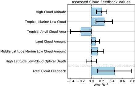
IPCC weights together the CRE’s of the various cloud types to arrive at the total positive CRE of 0.43W/sq.m.
As seen in the figure, only tropical anvil clouds are supposed to have a negative feedback, whereas all other cloud types are in the positive.
However, the positive CRE estimate for MARINE low clouds has lately been questioned in a big research project with field studies.
Strong cloud–circulation coupling explains weak trade cumulus feedback, Vogel et al, 2022, Nature.
https://doi.org/10.1038/s41586-022-05364-y
They claim that this very common and important cloud type is rather insensitive to warming, and should have a CRE around zero, and sometimes even negative. As you write “The main cooling occurs over the ocean, with an area-averaged cooling of -2.4 W/m2.”, and this is where IPCC errs with their positive estimate for marine clouds.
Thanks, Gibrahil. Excellent points, but not for this paper.
w.
The article appears to me to be logically flawed from the start. There is no way to demonstrate the existence of any feedback from a single set of measurements. The only way you can do so is to repeat the experiment a second time without the supposed feedback. Or you can present a convincing theoretical arguement that the result should be different.
Now in the case of the climate you state that over the 20th Century the earth has warmed by about 0.8 degrees. So without any other set of measurements it is impossible to know whether the earth would be warmer or colder without clouds. All you have done is shown how the cloud cover has responded to 0.8 degrees of global warming. What you have not done is shown that the earth would be warmer if the clouds behaved differently.
All of which means that unless you have a second earth without clouds it is impossible to experimentally determine whether or not clouds have a positive or negative effect.
Furthermore your statement that the earth has warmed by 0.8 degrees over a century plus your figures showing the large annual variations in temperature mean that your statement that
“as a long-term average for each gridcell, over thousands of years, the temperature and the corresponding cloud radiative effect have reached a steady state condition”
is incorrect. Clearly if the earth is warming and there are large annual variations then clouds and their radiative effects have not reached steady state conditions.
Furthermore the claim that a spatial comparision is equivalent to a temporal one does not appear to have any evidence to suuport it. If the earth is warming then it is possible that each place will respond differently and in sync with other places and so it might be posible
that every one of your grid cells will increase uniformly or that some warm and some cool or any other combination. And if the climate changes then the correlations you present will aslo change and thus cannot be used to make predictions about what will happen under a warming earth.
Finally Le Chatelier’s principle does not apply to the earth’s climate since it is not isolated. Rather it is driven by sunlight and there is a large (and roughly constant) flux of energy through the system which means that it is a driven dissipative system and its response cannot be predicted using Le Chatelier’s principle.
Izaak Walton September 1, 2023 10:22 pm
Let’s take the Greenland and Antarctic ice caps as examples. In those areas, as the temperature increases, the CRE becomes more positive, increasing the warming. This is positive feedback.
In the Pacific Warm Pool, on the other hand, as the temperature increases, the CRE becomes more negative. This is negative feedback, and quite strong feedback at that. And we have excellent evidence of that negative feedback, because said feedback is preventing the temperature of the Warm Pool from ever getting much over 30°C.
Regards,
w.
Willis,
How do you know whether the CRE increasing over icecaps is a feedback? You are now talking about two distinct local effects and it could be that CRE is increasing over greenland because the global temperature is rising or because the gulf stream strength is decreasing or any other of possible effects. The only way you can logically demonstrate a feedback is to rerun the experiment with the same forcing but with different potential feedbacks and see if you get a different result.
To be clear I am not trying to argue that the size and strength of the clouds feedback you discuss is wrong but rather that it is logically impossible to demonstrate the existence of a feedback from a single experiment. You need a control system that you can use to compare to the system with feedbacks before you can draw any conclusions.
If it is “logically impossible to demonstrate the existence of a feedback from a single experiment”, then why does my single experiment show strong negative feedback over the Pacific Warm Pool?
Because we know for a fact that there is strong negative feedback there, and that’s just what both of my methods show.
I’m not believing it’s just luck.
As to the icecaps, if it were a function of location then we’d expect to see very different results for Greenland and Antarctica. But as Fig. 5 shows, we do not see that. We see that in both areas, as temperatures rise the surface CRE becomes more positive.
Here’s another example, involving solar feedback by way of albedo. It shows the correlation of albedo and temperature.
In the areas where albedo and temperature are negatively correlated, as temperatures increase the albedo decreases. This is positive solar feedback.
On the other hand, in the mostly tropical areas where albedo and temperature are positively correlated, as temperature increases the albedo also increases, which reduces solar warming. This is negative feedback.
Here’s another example. I start driving a car, slowly increasing gas consumption. I graph the car’s speed against the gas use. I note that as I go faster and faster, it takes more and more gas to increase the speed by one mile per hour.
From this single experiment, I deduce that there is a negative feedback related to the speed. And if my single experiment is accurate enough, I can derive an equation showing that the negative feedback is some kind of power function of the speed.
So I’m sorry, but I don’t believe your claim about feedback.
w.
Willis,
you are confusing evidence of correlation with evidence of feedback. In all your examples all you have shown is that A and B are correlated. Correlations and feedbacks are logically distinct.
To take your example with the car how do you know that the engine does not have an inbuilt function to waste gas the longer it is driven for? Maybe the engine overheats over time and more energy is put into cooling it down? Again you could test this by running a control experiment in which you drove the car at a constant speed and monitored the gas usage.
Again from a single time series you cannot say anything about feedbacks. The only thing you can say whether or not two things are correlated. Demonstrating a feedback requires a control system (or theoretical model) for comparision.
What are you talking about?
You also can’t run a model plus or minus petrol to prove a point, or plus or minus cloud for that matter and pretend it is an experiment.
Experiments generate data not model outputs!
Bill,
that is exactly my point. A single experiment doesn’t generate
enough data to show the existence of feedbacks. To show that feedbacks exist you need a control that you can compare with.
Dear Izaak,
Running a model of a car with or without petrol does not prove anything about the car. Likewise running a model with or without cloud, CO2 or anything else. My point is that models do not produce data.
Thus, if derived data cannot be corroborated by observed data even at one point in time, the derived data are most likely wrong.
All the best,
Bill
You do realize that your argument works both ways. If you disagree with Willis’s examination of actual data showing negative feedback, then neither can climate science use positive feedback from clouds inside their models. It hasn’t been proven either way according to you. That makes all models using positive feedback worthless.
Climate modes are not useful when clouds are parameterized. Talk about correlation, the model will show exactly what the programmers wish.
By the way, you, don’t need a “control” system to prove feedback. A single, very simple experiment can provide sufficient data to arrive at a solution. Spit into a stiff breeze and the resulting data will provide a lasting example of what feedback can do.
Your “correlation” argument is a straw man argument. It is a generic statement that neither proves nor disproves the conclusion Willis has stated. Climate science has used “correlation” to assume CAGW is real and an existential danger. Why do you not argue that CAGW is also just correlation and not correct?
Jim.
You beat me to it.
Geoff S
Izaak Walton September 2, 2023 12:27 am
Willis,
you are confusing evidence of correlation with evidence of feedback. In all your examples all you have shown is that A and B are correlated. Correlations and feedbacks are logically distinct.
All of those are feedbacks, merely of different kinds.
w.
Willis,
you seem to want to define feedbacks in such a way that you can claim that everything is a feedback. Which then defeats the purpose. Roe in “Feedback, timescales and seeing red” stated
“In order to quantify the effect of a feedback, a reference system (i.e., a system without the feedback) must be defined. Defining this reference system is a central aspect of feedback analysis.”
So again the point is that if you want to claim clouds are a negative feedback you have to define the system without the feedback. And then you have to show how that system would have behaved when forced in the same manner as the system with feedbacks. And that is not possible if all you have is a single time series.
Thanks, Izaak. I think I see the difficulty.
The CRE is a direct measure of feedback, because it includes the feedback condition (clouds) as well as the reference condition (no clouds) into a single number.
In other words, the surface net CRE is the difference in total downwelling radiation between the feedback condition and the control condition.
And thus, your condition is satisfied.
w.
You do not need a control system. A system with a constant input should exhibit a constant output. Any change in output that is then driven back toward the constant output is a negative feedback. What is important is the time constant and value of the feedback. Non-linear systems and non-linear feedback are obviously more difficult to describe. Also, keep in mind that feedbacks can be multivariate, Clouds don’t need to provide the only feedback.
Willis,
I don’t get that:
Cheers,
Bill
If the albedo decreases as temperature increases (negative correlation), that lets in more sunshine—positive solar feedback.
w.
Dear Willis,
On re-reading, you say under “Final Thoughts that:
This does not explain how heat is lost from the closed system (in this case by forced or unforced advection “outside” of the cycle).
In the case of the tropical atmospheric heat pump, excess heat is expelled at the top of the tower directly as LW radiation to space. It is that part of the cycle that cools the column.
Residual cirrus cloud, which in your picture is streaming away from the head of the tower covers a larger area but has a smaller effect on blocking/scattering incoming SW than the gross loss of E from the tower itself. (Great photo by the way.)
Don’t forget too that the Hadley circulation shifts large amounts of moisture and embedded potential energy away from the tropics poleward to the mid-Latitudes. The point being, that it is not a picture, but a complex process.
All the best,
Bill Johnston
Well, actually no. The earth is not warming and indeed, data shows a feed-back mechanism operates across the true tropics. While I find the post is confusing (and somewhat contradictory), I don’t believe it is “flawed from the start”.
All the best,
Bill Johnston
http://www.bomwatch.com.au
Bill,
all global measurements show global warming. Whether satellite based or land based. Claiming that the earth isn’t warming is nonsense.
Dear Izaak,
Why is there a difference between ‘global measurements’ and temperature observed at Cairns, Townsville, Rockhampton, Gladstone, Amberley, Charleville, Rutherglen … and sites across the Pilbara region of Western Australia? You can check-out multiple analyses of individual datasets at http://www.bomwatch.com.au, and grab the data as well.
Also, why is there no trend in sea surface temperatures measured by Australian Institute of Marine Science dataloggers for up to 30 years at sites along the Great Barrier Reef? How come SST is no different now than it was in 1877 (https://www.bomwatch.com.au/bureau-of-meteorology/trends-in-sea-surface-temperature-at-townsville-great-barrier-reef/)? What drives people into believing something exists when it doesn’t?
Please tell me how ‘global measurements’ including satellite data show warming, when actual data do not. Given that satellites don’t actually measure temperature where do you think the errors and biases are?
I suggest for a start, look closely at Townsville (https://www.bomwatch.com.au/data-quality/climate-of-the-great-barrier-reef-queensland-climate-change-at-townsville-abstract-and-case-study/) or Halls Creek (https://www.bomwatch.com.au/bureau-of-meterology/part-6-halls-creek-western-australia/), then get back to me or leave a comment.
Yours sincerely,
Dr Bill Johnston.
http://www.bomwatch.com.au
Global temperature “increases” are calculated by using anomalies that are not based upon a common baseline. Neither are they temperature measurements. They are derived from temperatures, but are actually ΔT, a difference in temperature. Trending Δ values is not a good idea.
If you and I are driving a 10 MPH and I speed up to 12 MPH the mean is 10 MPH but the anomaly is 2 MPH. Did you speed up?
What Bill Johnson is trying to tell you is that there are locations which have zero change. To reach a 1.5 degree increase, you need to find offsetting locations that have increased by 3 degrees. There are too many locations that public data show have little or no warming. You want to prove something, find locations that have double the warming of the average. That is all it takes to prove the CAGW claim.
This is of some interest to me as, like you, I became frustrated with the ability of anyone in the academic side of this debate to work with the empirical facts of the whole Earth climate control system at a macro level, while being happy to play aroud in a fallacious game space define by the rabbit holes that all the partial and presumptive assumptions of modellers, so they are already in somone else killing zone or rabbit hole, cerated to trap them and ensure the observed triths are never allowed to dominate the debate.
Their models are created around a set of small perturbations using spurious presumtpions while avoiding the much larger feedbacks, and the natural changes we have measured many many times and they deny. So most academic realists i’ll intellectually fiddling while the planet burns, etc.
The way this has been engineered by the “consensual scientists”/ scientists without facts, is a deliberate distraction by a cleverer political cabal who control the narrative, that obvious trap should be obvious to smart and realist deterministic scientists but isn’t.
As Freeman Dyson pointed out, “its very simple”, “they’re wrong!” (My version…. It’s about the measurements, stupid!).
So how do we get to a straightforward empirical take down of the diversionary deceit of modelllers from what actually seen to happen by satellites, and communicable to lay people over the simple deceit od NASA’s corrupted terrestrial data and the db enial of the dominat controls andd nataural change by the false presumtions of their models, that are of no merit for any detrministic scientific purpose, because of the partial and presumptive bases they use to represent Earth’s climate system, as Nakamura and Clauson just pointed out so well, again.
So, in default of my cleverer peers, I am currently writing a simpler empirical assessment of the total natural feedback of the Earth control system that includes the overtly dominant feedbacks of clouds, also evaporation and Stefan Boltzmann LWIR radiation, in response to the dominant changes we no occur in response to changes in ocean surface temperature. So I looked for your key number regarding the cloud feedbackcomponent in your paper, which which was ultimately too dense for me to assess at speed, I am too thick perhaps, or blind, so I may have missed such a number in haste. Sorry if so and hence my question here ……………
Do you have a number for the long term average variability of cloud albedo, your short wave radiation reflection feedback per deg SST change for Tropospheric clouds? Or the same negative feedback quantified some other way?
FYI I estimate this negative feedback component at c.3.5W/m^2 per deg.
I have created these numbers in terms of the macro level NASA assessment of the changing thermal budget equilibrium, in terms of the essential and self evident mechanism of heat in = heat out energy balance driven by the primary control of changing SST that is planet Earth’s dominant climate control. Because these avoid the massive detail aggregation of regional climates as you have done, they already did it. Ny simple approach is designed to be hard to dismiss and simple to communicate to anyone who owns a car with air conditioning, and is outside the climate system science bubble,
NASA has carefully assessed the total radiation fluxes over a long period of satellite observations so they are well known, uncontroversial, and have escaped the gross abuse meted out to terrestrial temperature data ex-post by NASA climate alarmists, to make it better fit the political narratives. So my approach is more simplistic than yours, but I hope has merit in its conclusions.
My approach makes it possible to create simple empirical assessments of the variability of the dominant feedback components’ with temperature. Yours is more complex, but it appears we are both addressing the wildly presumptive mudellers’ guess that simply deny one of the overtly dominant negative feedback effects of the 67% of the planetary surface covered by clouds, mostly of the dense Tropospheric kind, which are mostly formed, and and thus dissipate most radiative latent heat of formation and also reflect most heat, at the equatorial regions, that varies significantly with ocean surface temperatures. All good.
Sod all happenes at the poles, scientifically speaking, except that, Earth’s heat circulation systems send the excess heat polewards, once the saturated tropical climate plateau is reached at around 30 deg SST, after which the heat spreads polewards, as when there were Hippos in Honiton at the Eemian event, when all three MIlanovitchcycles wre in phase 132.000 years ago, so that was a Doozy, as we scientists say.
My approach allows a first level scaling of the whole planetary system feedback effect from clouds, evaporation, and Stefan Boltzmann radiative loss, including variability in the positive feedback to SST change from changing water vapour GHE.
It’s easier to be clear and offers a high degree of certainty in scaling the total effect empirically, to compare with the small perturbations due to humans. Probably.
I will advise when ready. I was intending for it to be a paper but the simple fact, that you have discovered, is that scientific publishing has been taken over by the consensual science Cardinals of the climate Inquisition of the of the First UN Church of Climate Science, who brook no debate of their teachings, who the Sun revolves around whilst also shining our of their lying arses at the same time, will simply ensure any real deterministic science is suppressed without trace. And they are largely untroubled because their local activist clergy, who are the editorial gatekeepers of Scientific literature, will automatically reject the simple declaration of ANY measured empirical truth that suggests the “wholly wrong’UN church of modelling” may be wrong. A blasphemy, that can only be recanted, never be right.
First and last, I want to keep it accessible to lay people, perhaps even politicians, in an understandable way, Si the first attempt will be to simply publish as a book. It worked for Darwin. etc. Your work my offer a deeper dive into elements of the cloud feedbacl element. I suggest the rest are both self evident and also etsablished science, irrefutbable reality the UN narrative denies.
There is clearly a set of dominant natural control feedbacks that work at a scale that is untroubled by the tiny perturbations to the natural system by humans, and whose most proximal tipping point is towards the icing of the oceans, because the tropical oceans cannot easily warm above 30°, so the heat goes north and south. The real threat to life is the ice planet tipping point when it is possible all carbon based life could become extinct because CO2 falls below 150pp. But that another story, about a life-giving pollutant 😉
So…. What’s the feedback, Kenneth?
PS Sorry about the typos, again.
Dear Willis,
Figure 1 represents annual temperature swings for the concerning gridcells from monthly averages, if I understood correctly. These are result of seasonal effects, that’s why I’m confused about the figure for Average Global (14.8 according to figure). Shouldn’t it average out over each year and end up into the generally known 3°C global temperature swing?
Second question: what makes the difference of the numbers between figure 1 and 2 for each region? Perhaps you can also clarify a bit more where the wiskers and horizontal lines stand for in figure 2?
World Distribution of Temperatures. Air Temperature Data: what data are recorded? Daily Mean Daily Range Monthly Mean Annual Mean Annual Range. – ppt download (slideplayer.com)
To simplify: if the NH summer averages say 20C, and its winter averages 5C, while the SH winter is 7C and summer is 25C then the global average is 13.5C in NH summer and 15C in NH winter, so the global average only oscillates 1.5C while the seasonal hemispheric differences are much bigger at 15C and 17C, average 16C. Expand to gridcells.
You have to be very careful here. The variances of the temperatures are different in winter and summer. If that is no accounted from when doing “averages” you can get misleading results. A NH summer of 20C with a variance of 10C is different than a SH winter of 7C with a variance of 10C. The percentage differences are huge. tt’s somewhat akin to averaging the heights of Shetland ponies with the heights of quarter horses.
Trying to find a way to follow this thread….. by posting on it, no obvious button …..
New comments get entered in the text box just below the head post.
w.
Hi Willis,
You might try the Elsevier journal Earth and Planetary Science Letters. I don’t think they have a publication fee and they have one of the highest earth science impact factors.
Thanks,
w.
Powerful argument, with real data, that the net feedback from clouds is negative and therefore runaway global warming as the Alarmists claim is upon in in a few years is not going to happen
Willis’s thunderstorm work is also important. For that I have a metaphor that seems to help lay people:
If CO2 is like a blanket keeping warmth in the Earth’s system, it turns out to be a blanket with ten thousand holes.
Each tropical thunderstorm is a hole in the CO2 blanket. Heat is pumped through those holes, rising on the updrafts that cause those thunderclouds until the heat is above the CO2 and can escape into space.
If the Earth warms a little, the holes in the CO2 blanket grow in size and number.
All-sky LW λ ≈ −2 W m−2 K−1 is in agreement with the existing body of evidence.
CERES all-sky LW λ ∼−0.28 W m−2 decade−1
CERES decreased SW reflection (∼0.70 W m−2 decade−1)
Earth has a stabilizing feedback in the LW, but not in the SW.
all values ~± 0.2 W m-2.
In other words, an increasing greenhouse effect is cancelled by increased emission across the spectrum, including in the water vapour bands.
From hyperspectral obs https://www.nature.com/articles/s41561-023-01175-6/figures/1
Greenhouse effect is stable. Variability in energy accumulation is only in the SW.
Willis,
Just a nitpick but in presenting Fig 1 you call it the range of maximum temperature when I believe the plot if the range of maximum minus minimum.
This paper, like most great science papers, tends to bring up more questions than it answers. What better way to get people to think about what you are writing and pay attention.
I see great potential in the analysis you are doing in that, in my experience working with large data sets, the four distinct regions of Fig 5 indicates regions of different dominating effects where one or more effects diminish and others increase. This is obvious to anyone but you have the tools to perhaps quantify the effects and thus expand our understanding even further.
thanks for the great work and smooth sailing.
Bill
BCofTexas September 2, 2023 12:25 pm
Thanks, fixed.
w.
Just scanned your work, and found it refreshing, as usual. So nice to come across sanity in a modern world where the mental processes of so many (including myself) demonstrate a lack.
I’m curious regarding this observation: “In Fig. 3 we see that the clouds warm the poles and the deserts, and cool everywhere else.”
In my own experience this phenomenon is largely seen at night. In the desert the cooling is downright drastic once the sun goes down, (and at the poles once the sun goes down it stays down for months, of course). During such nights clouds are like a blanket, and slow or even reverse the cooling. However, during high noon (or high summer, at the Pole) it seems to me clouds cool the desert and the arctic slush.
Am I correct to assume that Fig 3 demonstrate that overall, (when you combine both daytime cooling and nighttime warming), the effect of clouds is a warming effect over desert sands and arctic sea-ice?
Yep.
w.
w – I hope you can get the final paper published in a less greedy journal. Here are my comments, use or ignore them as you wish:
– I didn’t follow “And as another example, over the entire 20th Century the temperature only increased by 0.8°C, which is a 0.3% temperature rise in 100 years.”. It looks like 0.8 over 100 years.
– You have two sections numbered ‘3’.