Guest Essay by Kip Hansen — 17 December 2022
The Central Limit Theorem is particularly good and valuable especially when have many measurements that have slightly different results. Say, for instance, you wanted to know very precisely the length of a particular stainless-steel rod. You measure it and get 502 mm. You expected 500 mm. So you measure it again: 498 mm. And again and again: 499, 501. You check the conditions: temperature the same each time? You get a better, more precise ruler. Measure again: 499.5 and again 500.2 and again 499.9 — one hundred times you measure. You can’t seem to get exactly the same result. Now you can use the Central Limit Theory (hereafter CLT) to good result. Throw your 108 measurements into a distribution chart or CLT calculator and you’ll see your central value very darned close to 500 mm and you’ll have an idea of the variation in measurements.
While the Law of Large Numbers is based on repeating the same experiment, or measurement, many times, thus could be depended on in this exact instance, the CLT only requires a largish population (overall data set) and the taking of the means of many samples of that data set.
It would take another post (possibly a book) to explain the all the benefits and limitations of the Central Limit Theory (CLT), but I will use a few examples to introduce that topic.
Example 1:
You take 100 measurements of the diameter of ball bearings produced by a machine on the same day. You can calculate the mean and can estimate a variance in the data. But you want a better idea, so you realize that you have 100 measurements from each Friday for the past year. 50 data sets of 100 measurements, which if sampled would give you fifty samples out of 306 possible daily samples of the total 3,060 measurements if you had 100 samples for every work day (six days a week, 51 weeks).
The central limit theory is about probability. It will tell you what the most likely (probable) mean diameter is of all your ball bearings produced on that machine. But, if you are presented with only the mean and the SD, and not the full distribution, it will tell you very little about how many ball bearings are within specification and thus have value to the company. The CLT can not tell you how many or what percentage of the ball bearings would have been within the specifications (if measured when produced) and how many outside spec (and thus useless). Oh, the Standard Deviation will not tell you either — it is not a measurement or quantity, it is a creature of probability.
Example 2:
The Khan Academy gives a fine example of the limitations of the Central Limit Theorem (albeit, not intentionally) in the following example (watch the YouTube if you like, about ten minutes) :

The image is the distribution diagram for our oddly loaded die (one of a pair of dice). It is loaded to come up 1 or 6, or 3 or 4, but never 2 or 5. But twice more likely to come 1 or 6 than 3 or 4. The image shows a diagram of expected distribution of the results of many rolls with the ratios of two 1s, one 3, one 4, and two 6s. Taking the means of random samples of this distribution out of 1000 rolls (technically, “the sampling distribution for the sample mean”), say samples of twenty rolls repeatedly, will eventually lead to a “normal distribution” with a fairly clearly visible (calculable) mean and SD.

Here, relying on the Central Limit Theorem, we return a mean of ≈3.5 (with some standard deviation).(We take “the mean of this sampling distribution” – the mean of means, an average of averages).
Now, if we take a fair die (one not loaded) and do the same thing, we will get the same mean of 3.5 (with some standard deviation).

Note: These distributions of frequencies of the sampled means are from 1000 random rolls (in Excel, using fx=RANDBETWEEN(1,6) – that for the loaded die was modified as required) and sampled every 25 rolls. Had we sampled a data set of 10,000 random rolls, the central limit would narrow and the mean of the sampled means — 3.5 —would become more distinct.

The Central Limit Theorem works exactly as claimed. If one collects enough samples (randomly selected data) from a population (or dataset…) and finds the means of those samples, the means will tend towards a standard or normal distribution – as we see in the charts above – the values of the means tend towards the (in this case known) true mean. In man-on-the-street language, the means are clumping in the center around the value of the mean at 3.5, making the characteristic “hump” of a Normal Distribution. Remember, this resulting mean is really the “mean of the sampled means”.
So, our fair die and our loaded die both produce approximate normal distributions when testing a 1000 random roll data set and sampling means. The distribution of the mean would improve – get closer to the known mean – if we had ten or one hundred times more of the random rolls and equally larger number of samples. Both the fair and loaded die have the same mean (though slightly different variance or deviation). I say “known mean” because we can, in this case, know the mean by straight-forward calculation, we have all the data points of the population and know the mean of the real-world distribution of the dies themselves.
In this setting, this is a true but almost totally useless result. Any high school math nerd could have just looked at the dies, maybe made a few rolls with each, and told you the same: the range of values is 1 through 6; the width of the range is 5; the mean of the range is 2.5 + 1 = 3.5. There is nothing more to discover by using the Central Limit Theorem against a data base of 1000 rolls of the one die – though it will also tell you the approximate Standard Deviation – which is also almost entirely useless.
Why do I say useless? Because context is important. Dice are used for games involving chance (well, more properly, probability) in which it is assumed that the sides of the dice that land facing up do so randomly. Further, each roll of a die or pair of dice is totally independent of any previous rolls.
Impermissible Values
As with all averages of every type, the means are just numbers. They may or not have physically sensible meanings.
One simple example is that a single die will never ever come up at the mean value of 3.5. The mean is correct but is not a possible (permissible) value for the roll of one die – never in a million rolls.
Our loaded die can only roll: 1, 3, 4 or 6. Our fair die can only roll 1, 2, 3, 4, 5 or 6. There just is no 3.5.
This is so basic and so universal that many will object to it as nonsense. But there are many physical metrics that have impermissible values. The classic and tired old cliché is the average number of children being 2.4. And we all know why, there are no “.4” children in any family – children come in whole numbers only.
However, if for some reason you want or need an approximate, statistically-derived mean for your intended purpose, then using the principles of the CLT is your ticket. Remember, to get a true mean of a set of values, one must add all the values together divide by the number of values.
The Central Limit Theorem method does not reduce uncertainty:
There is a common pretense (def: “Something imagined or pretended“) used often in science today, which treats a data set (all the measurements) as a sample, then take samples of the sample, use a CLT calculator, and call the result a truer mean than the mean of the actual measurements. Not only “truer”, but more precise. However, while the CLT value achieved may have small standard deviations, that fact is not the same as more accuracy of the measurements or less uncertainty regarding what the actual mean of the data set would be. If the data set is made up of uncertain measurements, then the true mean will be uncertain to the same degree.
Distribution of Values May be More Important
The Central Limit Theory-provided mean would be of no use whatever when considering the use of this loaded die in gambling. Why? … because the gambler wants to know how many times in a dozen die-rolls he can expect to get a “6”, or if rolling a pair of loaded dice, maybe a “7” or “11”. How much of an edge over the other gamblers does he gain if he introduces the loaded dice into the game when it’s his roll?
(BTW: I was once a semi-professional stage magician, and I assure you, introducing a pair of loaded dice is easy on stage or in a street game with all its distractions but nearly impossible in a casino.)
Let’s see this in frequency distributions of rolls of our dice, rolling just one die, fair and loaded (1000 simulated random rolls in Excel):

And if we are using a pair of fair or loaded dice (many games use two dice):

On the left, fair dice return more sevens than any other value. You can see this is tending towards the mean (of two dice) as expected. Two 1’s or two 6’s are rare for fair dice … as there is only a single unique combination each for the combined values of 2 and 12. Lots of ways to get a 7.
Our loaded dice return even more 7’s. In fact, over twice as many 7’s as any other number, almost 1-in-3 rolls. Also, the loaded dice have a much better chance of rolling 2 or 12, five times better than with fair dice. The loaded dice don’t ever return 3 or 11.
Now here we see that if we depended on the statistical (CLT) central value of the means of rolls to prove the dice were fair (which, remember is 3.5 for both fair and loaded dice) we have made a fatal error. The house (the casino itself) expects the distribution on the left from a pair of fair dice and thus the sets the rules to give the house a small percentage in its favor.
The gambler needs the actual distribution probability of the values of the rolls to make betting decisions.
If there are any dicing gamblers reading, please explain to non-gamblers in comments what an advantage this would be.
Finding and Using Means Isn’t Always What You Want
This insistence on using means produced approximately using the Central Limit Theorem (and its returned Standard Deviations) can create non-physical and useless results when misapplied. The CLT means could have misled us into believing that the loaded dice were fair, as they share a common mean with fair dice. But the CLT is a tool of probability and not a pragmatic tool that we can use to predict values of measurements in the real world. The CLT does not predict or provide values – it only provides estimated means and estimated deviations from that mean and these are just numbers.
Our Khan academy teacher, almost in the hushed tones of a description of an extra-normal phenomenon, points out that taking random same-sized samples from a data set (population of collected measurements, for instance) will also produce a Normal Distribution of the sampled sums! The triviality of this fact should be apparent – if the “sums divided by the [same] number of components” (the means of the samples) are normally distributed then the sums of the samples must need also be normally distributed (basic algebra).
In the Real World
Whether considering gambling with dice – loaded and fair – or evaluating the usability of ball bearing from the machinery we are evaluating – we may well find the estimated means and deviations obtained by applying the CLT are not always what we need and might even mislead us.
If we need to know which, and how many, of our ball bearings will fit the bearing races of a tractor manufacturing customer, we will need some analysis system and quality assurance tool closer to reality.
If our gambler is going to bet his money on the throw of a pair of specially-prepared loaded dice, he needs the full potential distribution, not of the means, but the probability distribution of the throws.
Averages or Means: One number to rule them all
Averages seem to be the sweetheart of data analysts of all stripes. Oddly enough, even when they have a complete data set like daily high tides for the year, which they could just look at visually, they want to find the mean.

The mean water level, which happens to be 27.15 ft (rounded) does not tell us much. The Mean High Water tells us more, but not nearly as much as the simple graph of the data points. For those unfamiliar with astronomic tides, most tides are on a ≈13 hour cycle, with a Higher High Tide (MHHW) and a less-high High Tide (MHW). That explains what seems to be two traces above.

Note: the data points are actually a time series of a small part of a cycle, we are pulling out the set of the two higher points and the two lower points in a graph like this. One can see the usefulness of a different plotting above each visually revealing more data than the other.
When launching my sailboat at a boat ramp near the station, the graph of actual high tide’s data points shows me that I need to catch the higher of the two high tides (Higher High Water), which sometimes gives me more than an extra two feet of water (over the mean) under the keel. If I used the mean and attempted to launch on the lower of the two high tides (High Water), I could find myself with a whole foot less water than I expected and if I had arrived with the boat expecting to pull it out with the boat trailer at the wrong point of the tide cycle, I could find five feet less water than at the MHHW. Far easier to put the boat in or take it out at the highest of the tides.
With this view of the tides for a month, we can see that each of the two higher tides themselves have a little harmonic cycle, up and down.

Here we have the distribution of values of the high tides. Doesn’t tell us very much – almost nothing about the tides that is numerically useful – unless of course, one only wants the means, which would be just as easily eye-ball guessed from the charts above or this chart — we would get a vaguely useful “around 29 feet.”
In this case, we have all the data points for the high tides at this station for the month, and could just calculate the mean directly and exactly (within the limits of the measurements) if we needed that – which I doubt would be the case. But at least we would have a true precise mean (plus the measurement uncertainty, of course) but I think we would find that in many practical senses, it is useless – in practice, we need the whole cycle and its values and its timing.
Why One Number?
Finding means (averages) gives a one-number result. Which is oh-so–much easier to look at and easier to understand than all that messy, confusing data!
In a previous post on a related topic, one commenter suggested we could use the CLT to find “the 2021 average maximum daily temperature at some fixed spot.” When asked why one would want do to so, the commenter replied “To tell if it is warmer regarding max temps than say 2020 or 1920, obviously.” [I particularly liked the ‘obviously’.] Now, any physicists reading here? Why does the requested single number — “2021 average maximum daily temperature” — not tell us much of anything that resembles “if it is warmer regarding max temps than say 2020 or 1920”? If we also had a similar single number for the “1920 average maximum daily temperature” at the same fixed spot, we would only know if our number for 2021 was higher or lower than the number for 1920. We would not know if “it was warmer” (in regards to anything).
At the most basic level, the “average maximum daily temperature” is not a measurement of temperature or warmness at all, but rather, as the same commenter admitted, is “just a number”.
If that isn’t clear to you (and, admittedly, the relationship between temperature and “warmness” and “heat content of the air” can be tricky), you’ll have to wait for a future essay on the topic.
It might be possible to tell if there is some temperature gradient at the fixed place using a fuller temperature record for that place…but comparing one single number with another single number does not do that.
And that is the major limitation of the Central Limit Theorem
The CLT is terrific at producing an approximate mean value of some population of data/measurements without having to directly calculate it from a full set of measurements. It gives one a SINGLE NUMBER from a messy collection of hundreds, thousands, millions of data points. It allows one to pretend that the single number (and its variation, as SDs) faithfully represents the whole data set/population-of-measurements. However, that is not true – it only gives the approximate mean, which is an average, and because it is an average (an estimated mean) it carries all of the limitations and disadvantages of all other types of averages.
The CLT is a model, a method, that will produce a Mean Value from ANY large enough set of numbers – the numbers do not need to be about anything real, they can be entirely random with no validity about anything. The CLT method pops out the estimated mean, closer and closer to a single value whenever more and more samples from the larger population are supplied it. Even when dealing with scientific measurements, the CLT will discover a mean (that looks very precise when “the uncertainty of the mean” is attached) just as easily from sloppy measurements, from fraudulent measurements, from copy-and-pasted findings, from “just-plain-made-up” findings, from “I generated my finding using a random number generator” findings and from findings with so much uncertainty as to hardly be called measurements at all.
Bottom Lines:
1. Using the CLT is useful if one has a large data set (many data points) and wishes, for some reason, to find an approximate mean of the data set, then using the principles of the Central Limit Theorem; finding the means of multiple samples from the data set, making a distribution diagram, and with enough samples, by finding the mean of the means, the CLT will point to the approximate mean, and give an idea of the variance in the data.
2. Since the result will be a mean, an average, and an approximate mean at that, then all the caveats and cautions that apply to the use of averages apply to the result.
3. The mean found through use of the CLT cannot and will not be less uncertain than the uncertainty of the actual mean of original uncertain measurements themselves. However, it is almost universally claimed that “the uncertainty of the mean” (really the SD or some such) thus found is many times smaller than the uncertainty of the actual mean of the original measurements (or data points) of the data set.
This claim is a so generally accepted and firmly held as a Statisticians’ Article of Faith that many commenting below will deride the idea of its falseness and present voluminous “proofs” from their statistical manuals to show that they such methods do reduce uncertainty.
4. When doing science and evaluating data sets, the urge to seek a “single number” to represent the large, messy, complex and complicated data sets is irresistible to many – and can lead to serious misunderstandings and even comical errors.
5. It is almost always better to do much more nuanced evaluation of a data set than simply finding and substituting a single number — such as a mean and then pretending that that single number can stand in for the real data.
# # # # #
Author’s Comment:
One Number to Rule Them All as a principal, go-to-first approach in science has been disastrous for reliability and trustworthiness of scientific research.
Substituting statistically-derived single numbers for actual data, even when the data itself is available and easily accessible, has been and is an endemic malpractice of today’s science.
I blame the ease of “computation without prior thought” – we all too often are looking for The Easy Way. We throw data sets at our computers filled with analysis models and statistical software which are often barely understood and way, way too often without real thought as to the caveats, limitations and consequences of varying methodologies.
I am not the first or only one to recognize this – maybe one of the last – but the poor practices continue and doubting the validity of these practices draws criticism and attacks.
I could be wrong now, but I don’t think so! (h/t Randy Newman)
# # # # #
Kip,
Your patience to write this essay is appreciated. No doubt, as you forecast, statisticians will make comments.
As I wrote to your earlier post, a central concept for statistics is to sample a population, so you can work with sub sets of the population. One seldom sees confirmation that one population is being sampled. A single population might be identified as one without significant influence of other variables affecting it.
Physicians use thermometers to get numbers for human body temperatures. Their population is the human population, here regarded as one population. The measured temperature is not influenced by the various designs of engineers.
Meteorologists use thermometers to get numbers for global temperature estimation. The result depends on engineered design.
Humans are part of the human population.
Thermometers in screens are individual devices whose properties vary so widely that they fail to be classed as a population when their numbers are grouped. They are not candidates for central limit or large numbers laws.
Physicians do not insert thermometers in patient A to measure the temperature of patient B.
My dislike for many aspirations of statistics in climate research is because of the improper ways that real uncertainty is made to look smaller than it is in practice. Bad outcomes are then permitted by appeals to the authority of statisticians. Geoff S
Geoff ==> Yeah, to be real and useful, averages (and CLT produces approximate averages) the data set must consist of “objects in sets to be averaged must be homogeneous and not so heterogeneous as to be incommensurable.”
Or, as I say above, not so vague and uncertain to barely be considered real measurements.
Physicians may not use a thermometer in one patient to determine the temperature of another, but the pathology labs do use the results gathered over time to determine the “normal” or reference range for those patients who utilised that particular laboratory which may differ from laboratory to laboratory for a wide range of reasons, both in-house procedures and external factors.
The variations are never discussed though. One of my jobs during COVID was to screen students coming to school. The variation was tremendous. Many were below the 98.6 and some significantly above on every check. The standard deviation was pretty large.
nonsense, variations are always discussed
Look! A comma!!
Perhaps he is recovering from his commaitis. However, his concurrent perioditis strain of punctuationitis and capitalizationitis are not showing any improvement.
That’s a classic example of spurious precision, having been converted from 37 degrees C.
And the 37 degrees C was originally the mid-point of a range, either 36 to 38 or 35 to 39 – too long since I read it, and didn’t pay much attention to an interesting piece of medical trivia.
cocky ==> I wrote something about body temperature in this essay.
I did a quick Google and found this:
Normal Body Temperature: Babies, Kids, Adults (healthline.com)
My own body temperature usually runs 96.8°F (my homeostasis function is dyslexic). If my temperature reads “normal” I’m courting a fever.
kalsel3294 ==> Physicians, and my father was one, use “normals” as a broad range to determine if one individual’s metric is way out of the normally expected range.
Many blood test metrics have normal ranges, and this is a good thing.
What none of these have is a single number to which all need conform. Even with the ranges, it is well recognized that many patients can have a number far out of range without having medical condition or needing treatment of any sort — Natural Variability.
And an important point is that in the practical application of such measurements, a precision of a tenth of a unit is meaningless when the range is several units.
Thank you for reminding us that most calculations involving a large data set produce “just a number”. I measure your rod with my tape measure, graduated in 1/16in, and get 19 9/16 inches which I like to write as 19.5625 inches because it’s much more accurate!
Exactly! The measurement is really only good to +/- half of 1/16″ (you know it’s not 19 1/2″ nor 19 5/8″ and can ‘eyeball’ a bit of precision tighter than that) which would be about +/- .03″ but the 19.5625 quoted above gives a false impression that the measurements are good to 10,000th of an inch.
One thing though, in climate science they can know the precision of the thermometers and tide guages, and then fret about some increasing trend away from the mean – but never considering that the trend is miniscule compared to the daily variation.
“The world is increasing in temp 1.5°C (or 3 or 5, etc) per century and therefore there will be mass extinctions and so on ”
And yet the biosphere tolerates 50°C swings in a year quite readily and generally seems to do better the warmer it is.
It like climate science can’t see the tree for the forest! Can’t see the real effects and benefits on actual living things because some global average is increasing – and like you point out, a false sense of precision is giving them an even more false trust in their doomsday predictions.
In particular when the “GAST” is an average of a COMBINATION of average daytime HIGHS and average nighttime LOWS, and most of the “increase” in the “average” temperature is an increase in the overnight LOW temperatures, NOT the daytime HIGH temperatures.
So exactly what species is going to be threatened with extinction or be forced to migrate to a new habitat because it doesn’t get quite as cool at night?!
But the “one number” statistical malfeasance allows such misperceptions to propagate. “The Earth has a FEVER!” Utter nonsense.
Maybe I’m misunderstanding something, but it doesn’t seem to me the author understands what the CLT is. We have phrases like “…by finding the mean of the means, the CLT will point to the approximate mean, and give an idea of the variance in the data”.
You don’t use the CLT to find a mean of means, and it doesn’t point to an approximate mean. The sample mean is the approximate mean, you don;t need the CLT to tell you what it is. What the CLT says, is that as sample size increases the sampling distribution tends towards a normal distribution.
You don’t have a clue do you? You sample a population with a given sample size and a large number of samples. You find the mean of each sample and write it down. All of the means from each of the samples forms a “sample mean distribution”. The mean of the “sample means distribution” is the ESTIMATED MEAN. The standard deviation of the “sample means distribution” is the Standard Error or SEM.
Why do you think Dr. Possolo expanded the standard deviation of the temperature sample in TN1900? It is basically because of the limited number of samples (that is, only one sample of size 22).
The sample size (number of elements in each sample) is important to insure you have IID samples. The size also determines how alike the deviation is in each sample which in turn makes the SEM more accurate. The number of samples determines the accuracy of the shape of the distribution.
I’ve tried to explain this to you many times, and I know you will never listen. But the problem is you, and Kip, keep confusing a description of what the CLT means, with the method of using it. You do not usually take a large number of samples in order to discover what the sample distribution is. You use the CLT to tell you what sort of distribution your single sample came from.
Taking multiple sample to get a better mean is not using the CLT to estimate the mean, it’s simply taking a much bigger sample, who h will have it’s own smaller SEM than the individual samples
“Why do you think Dr. Possolo expanded the standard deviation of the temperature sample in TN1900? ”
You keep asking me that, and then ignore my answer. He expands the uncertainty range to get a 95% confidence interval. It’s what you always do when you have a standard error or deviation or whatever. You multiply it by a coverage factor to get the required confidence interval. The size of the sample is irrelevant to this, apart from using a Student distribution rather than normal one.
he doesnt understand CLT and neither does gorman
The clown car has arrived, mosh, bellcurveman, bg-whatever can’t be far behind.
Mosher ==> I use CLT to represent the process of using the principle.
Holy schist! THREE capitalist letters!
Bell ==> I use CLT to represent the process of using the principle.
I’m not sure what you mean by that. My point it that you don’t seem to understand what the process is. You seem to be suggesting in the essay that the process is finding the mean of multiple means, and my point is that is not how you use the CLT.
I’m not objecting to you using simple examples rather than going into the proof of the theorem. I’m objecting to the use of strawman arguments to attack statisticians and scientists for doing things they don’t do.
Bell ==> The process is clearly explained and demonstrated in an app at onlinestatbook.com (for example).
Or, as explained here: “the sampling distribution of sample mean…This will have the same mean as your original distribution”
You may well have used different words to explain the process, but it is what it is.
Neither are explaining “the process” They are just demonstrating what the CLT looks like. I’m still trying to understand what you think the process is, and how it is used by statisticians and metrologist.
To me the sort of processes which make use of the CLT are when you take a single sample of reasonable size from a population, and then use the assumption of normality to test the significance of a hypothesis.
You seem to think that the use of the CLT process is to take thousands of samples of a given size and take the average of the average to get a less uncertain average.
How do you think anyone ever confirmed the theorem? Before assuming a normal distribution it’s a good idea to do a little legwork before applying the CLT willy-nilly.
It’s a theorem. You don’t need to confirm it. It’s proven.
Of course, it’s reassuring that you can run simulations to show that it’s correct.
Likewise, having spent years as a metrology tech (meter calibration, not weather monitoring) it continues to bug me greatly that people claim accuracy greater than the calibrated accuracy of an instrument simply by averaging values. Additionally, how many instruments you use does not matter if you are thinking in that direction. My experience in instrument calibration certainly showed me that the instrument uncertainty is essentially never normally distributed within the calibration specification window.
Gary W==> Yes. There is a continuing issue of confusing sample measurement distribution statistics – Mean, Standard Deviation, Skew, Kurtosis – which describe the variability of the sample data and the Measurement Uncertainty which describes the measurement instrument’s capability. The CLT deals with how sample size relates to variability (I.e. variance/standard deviation) in the sample and the population from which the sample is drawn. It has nothing to do with the measurement uncertainty.
The uncertainty of a mean of N samples is calculated as the instrument MU divided by the square root of N. Thus if the MU for a caliper is 0.01 mm then the MU of an average of 25 repeated measurements is 0.002 mm. This formula is derived from addition in quadrature of the MU’s of the individual measurements times a sensitivity coefficient. This is based on the fact that MU’s contribution to error in the measured results is random within the stated limits and thus multiple measurements will result in canceling a portion of the error.
I would note that in most all real world measurement processes the variability in a series of measurements as described by the Standard Deviation (e.g. 2-Sigma limits) is substantially larger than the MU of the average. If it is not, one should obtain a better instrument. I would further note that these comments apply only when dealing with well defined and controlled sampling and measurement methods. The error or uncertainty or any other characteristics claimed for data sets that are derived from different instruments, measurement procedures, sample selection and other highly variable conditions are indefensible. And that goes for the applicability of the CLT as well.
“The uncertainty of a mean of N samples is calculated as the instrument MU divided by the square root of N. Thus if the MU for a caliper is 0.01 mm then the MU of an average of 25 repeated measurements is 0.002 mm.”
People should read this twice. Let me add that the “repeated measurements” also means of the same thing. You can’t measure 25 different things, find an average, then claim you know the measurement of each thing to 0.002.
nope still wrong
You are not as smart as you think you are. If you were, you would realize that your down-votes indicate that people are not accepting your pronouncements. If you want to make your time investment worthwhile, explain exactly why you disagree with Jim and others. Your arrogant, drive-by ‘edicts’ are not impressing this group. Most are well educated, and are your intellectual peers. They provide logical arguments and often direct quotes from people who are actually experts, not someone who wants others to think he is some kind of expert.
Back in the 80s I played with temperature measurement and control while employed by a manufacturer of technological measuring equipment. Their temperature measurement equipment made ten measurements in a second or so, threw out any of those ten, 3 sigma or more from the mean, then presented the average of what remained as the temperature. I had to control a process at +/-0.1°F with a temperature dependent outcome variation. We seemed to be able to control the process, so the measurement system must have worked very closely to reality.
Steve ==> Of course, you are measuring basically “the same thing” many many times in a system with very little variation. The Law of Large Numbers thus is appropriately applied (especially when you throw away measurements “that you don’t like” (3 sigma more of the mean). I assume that the controlling equipment used that running mean to adjust the temperature in real time.
Quite simply, the system had to work….
“(especially when you throw away measurements “that you don’t like” (3 sigma more of the mean)”)
I’m guessing that the outlier rejection criteria was more based on previous data evaluation and sound engineering judgment than on “like”. That’s why they got the good results…
YES. There are no “series” of “repeated measurements” of the temperature, anywhere. There is only ONE measurement of temperature at a given moment at a given location (if there are any).
So we’ll never get greater precision by computing an average of such measurements.
AGW is Not Science said: “There is only ONE measurement of temperature at a given moment at a given location (if there are any).”
The ASOS user manual says all temperature observations are report as 1-minute averages.
So. does any climate scientist you can refer us to that actually uses that data to find an integrated value for an average, or do they all still use Tmax and Tmin.
Recording a 1 minute average is useless unless someone uses it to determine something.
Tmax and Tmin are themselves averages. That’s the point.
They are a one minute average, so what. What period of time does a MMTS average its readings over? How about an LIG? Do you think those are instantaneous readings? Ever hear of hysteresis?
Recall that this is the guy who thinks it is possible to determine and then remove all the “biases” in historical data.
The so what is that according to you and Kip that makes all temperature observations using ASOS and other similar modern electronic equipment useless and meaningless. Does it even make sense to argue about the uncertainty of a value you don’t think is useful and meaningful? Playing devil’s advocate here…wouldn’t the best strategy be to focus on that? Think about it. Since the law of propagation of uncertainty requires computing the partial derivative of an intensive value that means it’s result would have to be useless and meaningless as well. Again…assuming it truly is invalid to perform arithmetic operations on intensive properties. I’m just trying to help you form a more consistent argument.
My goodness, have you not read the multitude of posts denigrating using temperature as a proxy for heat? Tell us what the enthalpy difference is between a desert and marshland both at 70 degrees. Temperature is not a good proxy because of latent heat of H2O like it or not.
Are temps adjusted for height above sea level, i.e., the lapse rate? What is the difference in a temperature measured here in Topeka versus one in Miami, Florida at sea level due to the lapse rate?
Deflection and diversion. Enthalpy has nothing to do with this subthread. The fact remains that Tmin and Tmax are actually averages and you still think an average of an intensive property is useless and meaningless. If you want to argue that Tmin and Tmax are useless and meaningless than u(Tmin) and u(Tmax) would have to be useless and meaningless as well since the law of propagation of uncertainty requires doing arithmetic with Tmin and Tmax. Nevermind that you have stated many times that averages aren’t measurands which would have to mean that you don’t think either Tmin and Tmax are measurands. And if you don’t think they aren’t measurands then you probably don’t think u(Tmin) and u(Tmax) even exists.
So you have now proceeded to cancel those with whom you disagree. Good Luck. If you can’t beat them, cancel them. Why don’t you just admit that you have never had an upper level class, done research or designed anything needing to have true measurements. If you had you would appreciate the issues.
Zeke Hausfather is a serial abuser of the law of large numbers.
https://www.climateforesight.eu/interview/zeke-hausfather-every-tenth-of-a-degree-counts/
Well, let’s try a slightly different angle on CLT and uncertainty. Let’s assume you have made a large number of observations of a temperature value – perhaps of the water in a large tank. Your thermometer has one degree temperature marks. Furthermore, let’s assume the temperature does not change during your observation time and all temperature values you record are the same. (This is not unusual in the real world.) What does CLT tell you about the mean and uncertainty of your observed data? You certainly cannot use Standard Deviation of those observations to claim an uncertainty of ZERO for the tank’s water temperature. The uncertainty must always be equal to or greater than the measurement instrument’s calibration accuracy. Standard Deviation is not a substitute for instrument calibration accuracy.
Gary ==> “The uncertainty must always be equal to or greater than the measurement instrument’s calibration accuracy. Standard Deviation is not a substitute for instrument calibration accuracy.”
And it really is that simple — except for “stats and numbers” guys.
Sorry guys, if you follow the GUM or NIST with respect to Measurement Uncertainty you will find that any results derived through mathematical combination of multiple measurements follows this general formula.
uY = √[((δY/δx1)u1)^2 + … + ((δY/δxn)un)^2]
In this formula the δY/δx terms are the partial derivatives of the combining formula with respect to each measurement. These are referred to as “sensitivity coefficients”. The u terms are the uncertainties associated with the measurement. This formula is applicable to any result that involves calculation from more than one measurement. They can be different properties such as voltage times current to measure power.
For an average of multiple measurements the sensitivity coefficients are all 1/n and the u’s are all the same. Thus the combining formula for the MU of an average reduces to u/√n.
u=√n(u/n)^2) = √n(u^2/n^2) = u/√n
So averaging multiple replicate measurements does indeed reduce the uncertainty of the result. If it did not why would anyone want to bother with making repeated measurements? The argument that you can’t reduced MU through averaging assumes that every measurement is off by the same amount in the same direction. That is the definition of a systematic error, not measurement uncertainty.
“So averaging multiple replicate measurements does indeed reduce the uncertainty of the result. If it did not why would anyone want to bother with making repeated measurements? “
Interestingly, that is a bogus question. There are situations where averaging multiple measurements can be useful. For one, in some instances it can reduce noise. It’s been a few years but my recollection of the use of the NIST document you mention above is that it assumes the process measured is more accurately known than the instrument measuring it. Averaging repeated measurements provides an estimate of the instrument error from a known standard. Of course, that is generally useful only in instrument calibration labs.
Rick ==> Spoken like a true statistician. However, I am not talking “sensitivity coefficients” — I am talking just plain vanilla uncertainty of the original measurements.
Total uncertainty of uncertain measurements is ADDITIVE — and averaging is division.
Arithematic — not statistics.
See here.
If you can diagram — similar to the diagram I supply — a proof of your statistical formula, I’d like to see it here.
Use the same example — single digit +/- some equal amount.
Kip: What you have diagramed is not the uncertainty of the result, but rather a “sensitivity analysis” which simply asks what is the highest and lowest possible result within the uncertainty. But there is near zero probability that both measurements would deviate by the full uncertainty value in the same direction. Adding or subtracting results in a sensitivity coefficient of 1 for each value and thus the MU of the result is the square root of 2 = 1.414 if the MU is +/- 1.
Gary W: For all intents and purposes the variability in a series of repeated measurements is noise. That is why making multiple measurements and averaging produces a result with less uncertainty. It’s also why in the lab we do multiple replicate measurements and report the mean as well as the standard deviation and the Uncertainty of the mean. The SD and MU are not measures of the same thing. Often the SD is an order of magnitude greater than the MU. This is of particular importance when the measurement involves destruction of random samples such as steel coupons sampled from coil to determine tensile strength. The SD represents real variability between samples while the MU is a statement of confidence in the in the reported result.
Rick C ==> I diagram the real world uncertainty — not a probability. The diagram is a real world everyday measurement problem. Probability does not reduce uncertainty. The uncertainty is just there and doesn’t disappear because some of the range is “less probable” — which may be true, but it is still uncertain — which is why they call it uncertainty.
If you can diagram your solution to the simplest of everyday problems of averaging known measurement uncertainties and show that the “statistical approach” is a better understanding, have at it.
“The uncertainty is just there and doesn’t disappear because some of the range is “less probable” — which may be true, but it is still uncertain — which is why they call it uncertainty.”
But uncertainty, in the real world, is based on probabilities. Uncertainty intervals are defined by a probability range, e.g. the 95% confidence interval. Requiring 100% confidence in the range just makes the concept meaningless.
Bell ==> The uncertainty of rounded recorded temperatures is not a probability — it is a certainty — we know for certain what the range of the real world absolute measurement uncertainty is.
Uncertainty is not a probability when we know.
It’s odd to be requiring certainty about uncertainty. You want a meaninglessly large uncertainty interval, just so you can be certain it’s covered all possibilities, no matter how improbable.
Wrong—the probability distribution of a combined uncertainty is typically unknown.
If that were true, talk of an uncertainty interval is a meaningless sham. What use it it to know a result with an uncertainty of ±2cm if all that means is the value could be inside the interval or outside it, and you don’t know how likely it is to be inside? Why go through all the calculations if the result is just a bit of hand waving?
What is the probability distribution of a combined uncertainty spec for a digital voltmeter?
karlomonte: As a former manager of an accredited calibration laboratory, I can tell you that the answer to your question should be contained in the calibration certificate provided with the instrument. The certificate may even provide the calibration data and the uncertainty budget. Various components of the MU might be from normal, triangular or rectangular distributions. Each component has a “standard uncertainty” which is analogous to the standard deviation of a normal distribution. These standard uncertainties are combined as the square root of the sum of the squares (quadrature). This combined standard uncertainty is multiplied by a coverage factor (typically designated as ‘k’) equal to 2 for the 95% confidence MU or 3 for 99% confidence. This process is thoroughly described in technical detail with examples in the GUM which is the global standard that must be followed by. all organization providing calibration services. If you want to see an exhaustive treatment of the subject obtain a NIST calibration certificate for a primary standard reference.
You can challenge it all you want, but it is the process rigorously derived through international cooperation of standards bureaus and publishers such as ISO and NIST, and enforced by accreditation bodies such as ANSI, NVLAP, APLAC and ILAC.
Every independent laboratory, calibration laboratory and scientific instrument manufacturer is supposed to follow ISO 17025 which details calibration requirements including reporting of instrument MU in compliance with the GUM (ISO Guide to the expression of Uncertainty of Measurements.
Now, as me if the bulk of information being used by the climate change hysteria industry deals with MU correctly.
Hahahaha… NO.
Rick, you are of course quite correct, although in my ISO 17025 training I don’t recall having to report distributions, but only the work to calculate the combined and expanded uncertainties.
Typically the DVM manufacturer provides error band specs from which a combined uncertainty has to be inferred, specific to how it is being used. But the error bands have no statistics attached to them, not even the direction.
As the usual suspects here have finally revealed, they really don’t care about MU so it is quite pointless to argue these ideas with them.
Karlo: Yes, manufacturer’s specifications typically are very abbreviated. I most all cases you have to ask for an actual calibration certificate to get a proper MU statement. Many manufacturers charge extra for a CalCert. I’ve had cases where the charge for a calibration certificate was more than the price of the instrument.
There are also cases where calibration and determination of MU are not feasible using the normal process. The GUM and ISO 17025 allow for other methods to estimate MU based on things like experience and interlaboratory comparison studies.
If the uncertainty interval is +/-2cm, why do you say the value could be inside OR outside the interval? Does not the +/- value define the interval where the true value must be (barring a faulty instrument or faulty measurement, either of which is, it seems to me, a whole different thing).
How does that apply to averaging temperatures from different times in the day and from different locations with different devices?
I can measure temperature at one location at one time with an uncertainty of 0.1 C. The average global temperature might be something like 15C with a standard deviation of +/- 10C. That would indicate that ~ 95% of the measurements fall with a range of -5 to +35C. Given such a wide range in raw data, I’m not sure anything meaningful can be derived from the average. The measurement uncertainty of the individual measurements is trivial by comparison. Where global atmospheric temperature is concerned, there are dozens of reasons to doubt the validity of any claim. Fundamental problems include:
Sampling is not random.
Much of the earth is not sampled at all.
Frequency of measurements is inadequate to capture an integrated mean over a specified time period.
Instruments and measuring procedure are not standardized.
The “Global Mean Temperature” is not clearly defined.
A great deal of the data contained in various data bases has been adjusted or infilled based on comparison to other location and thus are not “independent” measurements.
All these issues violate sound scientific measurement practices and thus invalidate any claim of accuracy.
I do agree with everything you have stated here. The only thing I will add is that temperature trends should be done using time series analysis and not simple regression of very, very, sketchy data.
The only rationalization I can think of is that too many folks working on the Global Average Temperature are mathematicians that have no concept of how measurements are done in the real physical world. They have no appreciation for the problems you and Kip have mentioned.
If the same thing is measured by the same instrument and the thing being measured has a single, unique value.
If the samples have a bi-modal distribution, a more precise estimate of the mean of the samples may be useless if what one needs is an estimate of each of the mode’s values.
If a time series with a trend loses the sequence information, then it looks like a large variance that grows with time. The point being is that one can’t always depend on more samples providing more precision to a mean. One has to show some intelligence in handling the data.
In the example, the measurements are recorded to the nearest 1̊F. Unstated but necessarily true is that the ‘actual’ value is somewhere in the inclusive interval +/-0.5̊F around that reading.
If the measurements are all the same to some ̊F, then the water might actually be, for example -0.5̊F lower. Does using the calculations defined by the CLT get one closer to that actual temperature, with less uncertainty?
This, you state is systematic error but is that correct? It is within the basic uncertainty of the measurement. Can you get closer to the true temperature through any statistical or probability calculation?
The only thing you can reduce by multiple measurements of the same thing is random error. Those are errors whereby a minus error offsets a plus error. Technically, one should graph the errors to see if they have a Gaussian distribution.
The problem one has with uncertainty is that each measurement, even those with error, has an uncertainty. So, one doesn’t really know if the errors cancel each other out. In other words, uncertainty builds. It is one reason for an expanded standard uncertainty.
Andy: I said that if an instrument is always off by the same amount in the same direction that is systematic error and is not subject to the CLT. This might occur for example in an old style thermometer where the glass tube is attached to an scaled metal plate. If the plate should slip down relative tube all readings will be off by the same amount.
Systematic error exists to some degree in almost all measurements but often it is identified in calibration and applying a correction then eliminates it. But an unrecognized systematic error is not accounted for in MU statements for the simple reason that it is unrecognized.
You are mixing instrument resolution (the smallest readable difference) with uncertainty and systematic error. Resolution is always one component of uncertainty – taken as 1/2 the smallest division. Other components must also be included such as the uncertainty of calibration references.
Rounding to the nearest marking introduces a half-interval plus/minus. However, there is also an uncertainty introduced from the inability to determine 0.49 from 0.50. Consequently, some measurements are rounded up that should have been rounded down, and vice versa, some are rounded down that should have been rounded up. I suspect this is why the NWS specified a +/- 1 degree.
And how many weather “thermometer readings” fit this “repeated measurements” description? None.
Gary W ==> Thank you for the report from “the guy who actually does things” — which is opposed to the guy who studied stats in uni.
Additionally, something that is being measured has to have a unique value that doesn’t change with time (stationarity). Furthermore, if what is being measured has a large variance, increasing the precision of the mean has little practical value because it spreads out the probability bounds to the extent that the extra ‘significant’ figures have little utility.
Clyde,
That is an excellent point. From my engine rebuilding days as a youth, this is an important fact in high compression engines. One must measure the cylinder bores multiple times at different locations and be sure that the inside micrometer is reading the maximum measurement each time. One must be sure that the high spots and low spots can be sufficiently covered by the compression rings or blowby will occur. Measurement uncertainty abounds.
It always slays me when people think that uncertainty when measuring different things will cancel. I liken it to saving old brake rotors in a pile, and when working on one car, you go measure a whole bunch of the saved ones along with the one you are considering, to arrive at an accurate measurement. The real world just doesn’t work that way. You have to measure the SAME thing multiple times.
The example in the opening paragragh is an example of determining the accuracy of the measuring device. The mean length of the rod can only be expressed as 500mm +- 2mm. Using the old spring style kitchen scales is a good example of getting a different weight each time the same item is weighed.
Example 1 is a different situation with that used to measure the ball bearings already having a known accuracy, it is measuring the variation in the production process.
Except, each measurement also has uncertainty that is contributed by the measuring device. As you say the same instrument can give different readings each time you measure the same thing. That is part of the quality process, understanding when the measuring device is showing variation and when the manufacturing process itself is introducing variation.
kalsel3294 ==> Welcome to the conversation, don’t recognize your commenter-handle (but that may be my oldster memory). This is your second comment here to this essay.
Meauring the stainless steel rod, in the real world, is a guy attempting to get a good measurement of his SS rod expecting it to be 500 mm. Correctly, he must decide to report 500 mm +/- 2 mm as you suggest. Hopefully, that is good enough for him and his superiors or customers. For the Mars Rover Project, a total failure though.
Example 1, ball bearings, is NOT measuring “ball bearings already having a known accuracy”….that is what the measuring is meant to accomplish. Sorry if this was not clear.
“The Central Limit Theorem is particularly good and valuable especially when have many measurements that have slightly different results.”
Totally confused, as many here, about what the CLT is. From the Wiki link:
“In probability theory, the central limit theorem (CLT) establishes that, in many situations, when independent random variables are summed up, their properly normalized sum tends toward a normal distribution even if the original variables themselves are not normally distributed.”
It’s important, but the surprising result is convergence to a normal distribution, not convergence to the mean. The latter is the result of the Law of Large Numbers, and it applies under the same conditions as CLT; in fact it is a corollary of it.
sed ‘s/[Cc]entral [Ll]imit [Tt]heorem/Law of Large Numbers/g;s/{Cc]{Ll][Tt]/LLN/g” $infile > $outfile
Simples 🙂
Hmm, that joke seems to have gone down like a lead balloon 🙁
old cocky ==> Gee, you’d have to explain it to me — I had no idea it was a joke — didn’t mean a thing to me….
You had to be there…
And to add the most important aspect of the CLT: it allows comparison between two different datasets to assess the probability they come from a single population.
In other words it is a key element of statistical testing and inference.
I would suggest people go and read Statistics and data analysis in geology by John C. Davis.
Then try geostatistics and particularly the concept of a random function and the difference between kriging and simulation and why both are important to understanding uncertainty.
ThinkingScientist ==> don’t get me started on the idiocy of krigging temperatures……
If kriging isn’t your thing then how do you propose forming a scalar (or vector) field from a set of data point?
What are your thoughts on NIST using kriging in TN 1900?
Same old, same old. Try to stay on the subject at hand instead of deflecting to something else. I don’t remember seeing krigging mentioned anywhere in the GUM when discussing measurement uncertainty.
Dude, do the mass fractions measured in sediment change on a second by second continuous basis like temperature?
I never mentioned kriging temps. I am talking about understanding of underlying principles.
Like using a thermometer on the east coast of Greenland plus one in Nova Scotia and one on Ellesmere Island to report the ‘average’ temperature of Greenland?
It’s important, but the surprising result is convergence to a normal distribution,
====$$
On this point I agree. As I state in more detail further on, it is my conjecture that this convergence to the normal distribution that has led a generation of climate scientists to falsely believe that temperature records have predictive power
It is the same problem as predicting the stock market from the dow. When the dow is going up it is a safe bet the market will be up tomorrow. Until it isn’t.
Temperature is a time series at its base. What climate science has tried to do is grab onto some measurements that were never designed to be able to be used for trending over a long term. I have developed myself too many graphs showing Tmax stagnant and Tmin growing to believe that land temperatures are going to burn us up. Others have posted the same.
Climate science needs to start explaining how the increase in Tmin is going to affect the earth. I have seen several studies from the agriculture community where growing degree days have increased thereby allowing longer maturing varieties that have better yields. Warmer nights mean less heating. On and on.
Part of the reason some are denying the accuracy of what is being done is having to admit that past temperature data is not fit for use. Man, that a big apple cart to upset.
HVAC folks have moved on to using integration of the latest minute based temperatures that are available for more accurate computing of heating/cooling degree days. You would think climate science would be doing the same since we now have decades of this kind of data available.
Certain trees, such as apples and cherries, do have minimum cold hour requirements.
“I have developed myself too many graphs showing Tmax stagnant and Tmin growing to believe that land temperatures are going to burn us up. Others have posted the same.”
Here’s my graph based on BEST maximum and minimum land data.
Min temperatures have gone up more since the 19th century, but since 1975 max temperatures seem to be warming faster.
Who am I to disagree, but I certainly can’t detect any warmer in the winter nights here?
From:
https://www.probabilisticworld.com/law-large-numbers/
The term ‘probabilistic process’ is defined as the probability of something occurring in a repeated experiment. The flipping of a coin is a probabilistic process. That is, what percentage of the time does heads or tails occur. Rolling a die is a probabilistic process when you are examining how often each number occurs. So fundamentally the LLN deals with probabilities and frequencies in a process that can be repeated. It is important that the subject remain the same. For example, if I roll 10 dice 1000 times and plot the results, it could happen that I will have different frequencies for the numbers 1 – 6 because of differences in the dice.
Can this weak LLN be applied to measurements? It can under certain conditions. Basically, you must measure the same thing multiple times with the same device. What occurs when this happens? What is the distribution of the measurements? What happens is that there will be more of the measurements in the center and fewer and fewer as you move away from the center. In other words a normal or Gaussian distribution. The center becomes the statistical mean and is called the “true value”. Why is this? Because small errors in making readings are more likely than large errors. As a result, a Gaussian distribution will likely occur where there are equal values both below and above the mean which offset each other and the mean is the point where everything cancels. The above is a description of the weak LLN.
The strong LLN deals with the average of random variables. The strong law says the average of sample means will converge to the accepted value. However, in both cases these laws must meet what is known as Independent and Identical Distributions (IID).
What does identically distributed mean? Each sample must have the same distribution as the population. For example, you have a herd of horses and you want to find the average height. But, the herd is made up of Clydesdales, Thoroughbreds, Welsh Ponies, and Miniatures. You wouldn’t go out and measure only Welsh Ponies and Miniatures in some samples and only Clydesdales in other samples. In other words your samples would not have identical distributions as the population.
Remember, X1, X2, X3, … are really the means of each of various samples taken from the entire population. They are NOT the data points in a population. This is an extremely important concept. Many folks think the sample means and the statistics derived from the distribution of sample means accurately describe the statistical parameters of the population. They do not! If sampling is done correctly, the sample mean can give a direct and fairly accurate estimate for the population mean. However, the standard deviation of the sample means IS NOT a direct estimation of the population standard deviation. Remember, the distribution of the sample means is a DERIVED value from sampling the population. It will not resemble the variance of the population. It must be multiplied by the square root of the size of the samples taken (not the number of samples).
Open a new tab and copy and paste this
http://www.ltcconline.net/greenl/java/Statistics/clt/cltsimulation.html
Click user and draw the worst population distribution you can, then select different sample sizes to see what the sample means distribution looks like.
Then do the same and go to this site.
https://onlinestatbook.com/stat_sim/sampling_dist/index.html
And when a large error does occur, it is likely to be a problem of transposing digits or an electrical noise spike. These then end up being discarded as outliers.
Closely followed by the Nitpick Nick Shuffle…
Nick ==> It is the use in practice that concerns me — and in practice, CLT is used to excuse confusing the convergence to a normal distribution with its centralized mean and to add some sort of meaning to its SDs. — this result is NOT surprising at all. That is the magical thinking — CLT methodology requires the result and gets the result from any sort of large collection of mere numbers.
Since it does this with any sort of collection of numbers — it must be used very carefully and not be confused as transferring any significance to the data set.
The key word here is, “sum.” The CLT is about the distribution of the sum of many independent random variables. But note that word, “independent.” If the random variables are correlated, the CLT doesn’t apply.
If the CLT does apply, the distribution of the sum will tend toward a normal (Gaussian) distribution, the mean will be the sum of the means, and the variance will be the sum of the variances.
The big “limitation” is in the independence. Lots of things are not independent or, more likely, cannot be known to be independent.
Note also that even when the CLT doesn’t apply the mean of the sum is still the sum of the means. The mean of the sum of a number of random variables is always the sum of the means. This is NOT the law of large numbers.
You can work through any example of just two random variables and see that the mean of the sum is always the sum of the means. For example, take a random variable that’s 0 half the time and 1 half the time. The mean is 1/2. Suppose we have second random variable that’s perfectly correlated with the first one. It’s 0 or 2, 0 when the first variable is 0 and 2 when the first variable is 1. The second variable’s mean is 1 (0 half the time and 2 half the time). The sum of the means is 1.5, but note that the sum of the two random variables is either 0 or 3, each half the time, also yielding a mean of 1.5
Now let the second random variable be perfectly negatively correlated, so that it’s 2 when the first variable is 0, and 0 when the first variable is 1. Now the sum is 1 half the time and 2 half the time, and the mean is still 1.5
One final note. A theorem about the sum of random variables teaches us nothing about the quality of the individual variables that have been summed. You may call that a “limitation” if you like.
Regarding this CLT description, what would a “properly normalized sum” be of thousands of different temperature measurements made in thousands of different places by thousands of different thermometers of varying accuracy?
A lot of this implies making a reading with one instrument. How do you accommodate readings with different instruments? And never reading the same thing with these different instruments.
I’m asking if the statistics have to be run differently, if say, I read 1000 items and use 4 different instruments to get my data.
Real world operating practices vs desktop theoretically perfect situations Alexy?
Alexy ==> It is important to know that we are dealing with statistical animals here. Statistics has its place — but in practice is more often substituted for thinking.
The Central Limit Theorem is an observable phenomenon dealing with large sets of numbers (any numbers).
The Law of Large Numbers (LLN) (two versions) mostly deals with lots of measurements of the same thing (see Jim Gorman’s comment above).
In your example, I wouldn’t try to use the LLN but could consider all of the measurements as a single data set (“My Measurements of my item”) apply the principles of CLT, and get a distribution of the means, find the means of those samples, and settle for that. You will have an approximate mean of all the measurements and some variance.
Don’t confuse your finding as the real mean or what statisticians call “the true mean”.
We should ignore statistics for a moment and consider the sources of instrument error.
1 – sixty students measure something with the same ruler
2 – one student measures the same thing with sixty different rulers
3 – one machinist measures the same thing with a micrometer
The rulers have different thicknesses. That changes the parallax error.
There are predictable human errors. If the thing being measured is precisely one inch thick, the average of the sixty student measurements will probably be one inch. If the thing is 1.01 inches thick, the average of the sixty student measurements will probably still be one inch.
If I’m setting up four production lines and have four properly calibrated test instruments of the same type, any variability will be due to the production lines, not the test instruments.
On the other hand, if I’m taking field strength measurements for an AM radio transmitter, I have to realise that I won’t get the same measurement even later on the same day.
So, the answer to your question depends on what you’re measuring and why you’re measuring and what you intend to do with the results.
Commie ==> Thanks heavens for persons who realize that “context matters”.
In many cases, the “context” that is missing is “…in the real world.”
“The mean found through use of the CLT cannot and will not be less uncertain than the uncertainty of the actual mean of original uncertain measurements themselves.”
I’m not quite sure what this means.
However, the standard error of the sample mean really is smaller than
(1) the standard deviation of the sample; and
(2) the measurement error.
It is generally not advisable to contest mathematics with words.
None of Kip’s homespun statistical theories are presented with any mathematically precise and rigorous descriptions and proofs using techniques described in text books and peer-reviewed journals. Understandable, given as far it appears, he has no formal training in statistical theory and falls back on being just a “science journalist” (or more correctly “science blogger”). What is not understandable is his level of dogmatism that he is unassailably correct despite the above lack of mathematical rigour. What is also hard to understand is why WUWT is hosting this statistical “snake oil” without at least some subject-matter expert review. I have been a reviewer for applied statistics and application-specific journals and published myself many times in this area over 45 years and I can tell you that these essays would not even make it to the review stage without the prerequisite mathematically explicit descriptions and proofs.
A rigorous mathematical proof can only be properly evaluated by a rigorous mathematition, on average 99 time out of 100.
Case in point. Does the Law of Large Numbers apply to future temperatures? For LLN we need a constant mean and variance, such as a coin. Many overlook this requirement and assume LLN applies everywhere.
Thus our question can be answered both yes and no.
No, because we know from paleo temperature data that mean temperature and variance are not constant.
Yes, because if one looks at the entire paleo record one can calculate a mean and variance that for all intents and purposes will not change over a span of a few thousand years.
Which one of these is true?
steve_showme
It is likely that WUWT staff will welcome your written essay on the subject. They accepted three of mine in September. Why not go for it? Geoff S
Geoff. Thanks for that idea. I generally like reading WUWT on subject areas I have no professional expertise in, like energy economics, policy, battery technology, climatology etc and news articles with comments such as those posted by Eric Worrall. I enjoy reading those and follow-up links to articles and getting informed. I just do not get the point of these statistical theory “lectures” by Kip especially when they are presenting false assertions as far as “false” can be gleaned from the maths-free homespun “theory” presented. The links given are web articles and not text books or peer-reviewed journal articles and these web links tend to be maths free as well.
I like to think I can make a better contribution in the peer review literature, even if its less sensational which applied statistics usually is unless its this type of “ALERT: the experts have had this wrong all along!” article.
I believe I have helped push back against the alarmist narrative (“Blue Planet”, Greta’s “ecosystems are collapsing…” etc) that Antarctic krill populations have catastrophically declined over the past 4 decades.
10.9734/arrb/2021/v36i1230460
https://environments.aq/publications/antarctic-krill-and-its-fishery-current-status-and-challenges/
and called out poorly designed studies from a statistical power standpoint
10.9734/cjast/2022/v41i333946
I can open all but your first “pushback against the alarmist narrative”. Any ideas?
Notably silly clicking. Even for here. I aksed for help opening the only link I was having trouble with. Apparently there’s some click first (based on the poster), don’t aks questions later posters lurking…
Bib ==> the numbered IP addresses don’t work for me either.
Thanks for your attention. Just one of those things….
Use Google Scholar for the DOIs and for the DOI 10.9734/arrb/2021/v36i1230460 use the first version GS links to.
Thanks steve. If your evaluative critiques are correct, then this would certainly be the best way to out claims made with improper evaluative techniques. I read WUWT articles per the Seinfeld Kramer effect*, but prefer superterranea for actual science and technology advancement…
*“He is a loathsome, offensive brute. Yet I can’t look away.”
Sorry dude, you have not shown that any of the claims are in “false”.
The main driver here is the fact that there are temperature values in “anomalies” that far, far exceed the resolution of readings and records. Prior to 1980, temperatures were read and recorded as integers. Showing variations with 2 or 3 decimal places just doesn’t compute with those of us have dealt with measurements in industry where this would not be allowed, either ethically or legally. Trying to use statistics to justify this is both incorrect and inept.
Resolution in measurements conveys a fixed amount of information. Adding more information in the form of extra significant digits is writing fiction, no matter how you cut it. It is what Significant Digits were designed to control and what error bars are supposed to show.
If you have a way to increase resolution of measurements through mathematics and statistics most of us would be more than pleased for you to post the mathematics behind it. Most of us would enjoy purchasing less expensive measuring equipment and instead use a computer to add the necessary resolution.
A couple of caveats you must deal with though. First, temperature is not a discreet phenomenon. It is an analog continuous function. It is a time series with very, very sparse and generally highly uncertain samples.
And the variance isn’t always noise. Often it is just high-frequency variations associated with turbulence and wind gusts, associated with the passage of air masses of different properties.
Also, one can, as I have, see fairly consistent large temperature differences for different but not widely located locations. Temperatures, for climate purposes, are reported as a single value derived from single location, or homogenized from a number of different locations, that may well be very different from any of the measured temperatures or any average of those measured temperatures. It is rather like an extreme version of reported urban/rural differences.
Also it would be very difficult to write a technical response to this article since without the precise mathematical expressions and exposition of these in the text its hard to be sure exactly what Kip is proposing and what statistical methodology he is relying on. That’s if I was even motivated to wade through it all which I am not since I have better things to do in my semi-retirement like gardening, sport (mostly watching actually talented sports-people), consulting and publishing peer reviewed papers.
If you need the necessary documents, there are several.
NIST has several Technical Notes on uncertainty in measurements as does NIH.
Dr. John R. Taylor’s book, An Introduction to Error Analysis is a good starting point.
JCGM 100:2008, Evaluation of measurement data — Guide to the expression of uncertainty in measurement is perhaps the “bible” most of us start with. You will want to read Annexes B, C, and D for a good basis in physical measurements.
Perhaps reference to the first article of this series would bring a little clarity.
https://wattsupwiththat.com/2022/12/09/plus-or-minus-isnt-a-question/
It seems peculiar to me that Kip did not provide a link at the beginning of this article.
steve-showme,
C’mon now, why not give it a go. If you are worried about audience comprehension, some WUWT readers are educated rather well. Not me, I just did the advanced option of both Pure and Applied Mathematices III at uni as part of an ordi=nary Science fegree. Others are much wiser.
If it encourages you, I can suggest a topic. It is about measurement and interpretation of surface sea temperatures, SST. Here are the basic from Kip’s previous post here.
…………
It is unclear what the purpose of uncertainty estimation is. To illustrate this, I use the example of measurement of sea surface temperatures by Argo floats. Here is a link:
https://www.sciencedirect.com/science/article/pii/S0078323422000975
It has claim that “The ARGO float can measure temperature in the range from –2.5°C to 35°C with an accuracy of 0.001°C.”
I have contacted bodies like the National Standards Laboratories of several countries to ask what the best performance of their controlled temperature water baths is. The UK reply is typical:
National Physical Laboratory | Hampton Road | Teddington, Middlesex | UK | TW11 0LWDear Geoffrey,
“NPL has a water bath in which the temperature is controlled to ~0.001 °C, and our measurement capability for calibrations in the bath in the range up to 100 °C is 0.005 °C.”
Without a dive into the terminological jungle, readers would possibly infer that Argo in the open ocean was doing as well as the NPL whose sophisticated, world class conditions are controlled to get the best they can. It would be logical to conclude that the Argo people were delusional. It is only on deeper study that you start to find why things are said.
………………………..
Steve, why not help us with some deeper study and do that dive? After being a commentor on WUWT since it began (almost) I think that I can read the mood that your input would be welcomed. Geoff S
The issue, in my opinion, has nothing to do with statistical rigor. Temperatures on earth are provably NOT ‘normally distributed’. They vary daily, monthly, annually, spatially, by the decade, century, millennium, any other period or location that has a name. They vary so much that in almost every case, the precision of the measurement instrument is generally far better than the variation in whatever is being measured.
This is compounded by the fact that it’s quite easy to ‘read a thermometer’ (or any other device that outputs a ‘temperature’ number), but it’s quite difficult to measure an accurate temperature. This is because the value shown by the instrument is influenced by radiation, conduction, and convection to and from whatever is being measured.
What is generally unknown in all of this, is the variation in whatever is being measured. That, in fact, is the problem. Is the earth warming or is it cooling? That’s certainly debated. Arguing statistics won’t answer that question. The largest percentage gain in information happens when the sample size goes from zero to 1. It doesn’t take statistics to analyze that.
More sampling and statistics can only prove that it was wrong.
Tom: The Central Limit Theorem is not a hypothesis. It is, as the name suggests, a Theorem. It is not a conjecture, either, or as Kip suggests, a theory. The Central Limit Theorem is true.
The Central Limit Theorem does not state that temperatures are normally distributed, and the fact that temperatures are not does therefore not disprove the Central Limit Theorem.
The Central Limit Theorem (or rather, the later mixing extensions of the CLT) does state that the distribution of the average temperature converges to the normal distribution.
I have no doubt that the averages of ensembles of temperatures measured somewhere, at sometimes trend toward a normal distribution. To me, that is not relevant to: “Is the earth warming, or cooling?”
I also would argue that the actual distribution of temperatures within the samples might help lead to insights that help answer the question.
Richard ==> “CLT does state that the distribution of the average temperature converges to the normal distribution.”
Yes, of course it does! It MUST — it will return the same result for ANY (literally any) large set of numbers — it means absolutely NOTHING then that it does so for temperatures numbers.
It certainly (and demonstrably) does not show that temperatures themselves re normally distributed.
“It will return the same result for any large set of numbers”
It does not.
Yet the data values nor their uncertainties do not change do they? Can a sum divided by a constant or taking a square root of a non-perfect square allow one to increase the resolution of the temperatures on which the calculations are based?
Are physical labs at universities all incorrect in saying you can’t do that?
Yes, it can. Measurement error is random and cancels out with repeated measurement.
All measurement error is random and cancels?
How do you know this?
You first must recognize and acknowledge that error and uncertainty are two different things. Each repeated measurement has both error and uncertainty. If one can show that the distribution of measurements IS normal, they may cancel but they may not due to uncertainty. For example, I make two measurements, one 1.0 and the second measurement is 1.1. The mean is 1.05 and I assume that random errors cancel and the true value is 1.05. But, the uncertainty in each measurement is ±0.05. Does the uncertainty also cancel just because the error portion does?
The first measurement can vary from 0.95 to 1.05 and the second from 1.05 to 1.15. Uncertainty in each measurement means you don’t know the EXACT value. What is the uncertainty in the average?
“For example, I make two measurements, one 1.0 and the second measurement is 1.1. The mean is 1.05 and I assume that random errors cancel and the true value is 1.05.”
That’s not what cancellation means. nobody claims that everything will exactly cancel out and the error will be zero. That’s why the uncertainty, assuming independence, will be 0.05 / sqrt(2) ~ = 0.035.
Tom Johnson ==> Yes, as always, pragmatism trumps statistical dogma.
Since the “increase in temperature” is based on hundredths or thousandths of a degree, it is appropriate to question just how these values are calculated and if they are accurate. If someone says they know the temperature increase from 1920 to 1921 is 0.2 or even 0.25 degrees, when the temperatures were all recorded as integers, I would like to know how this resolution was obtained through statistics.
Yes, the tail on the cold side is longer than the hot side.
Your diatribe includes no specific information about why you believe Kip’s explanation, which is appropriate for lay people, has inaccuracies. As someone who “I have been a reviewer for applied statistics and application-specific journals and published myself many times” you should then have a good basis for pointing out errors, but you have said nothing concrete.
Many of us have dealt with measurement uncertainty in numerous fashions in various industries. If you want to point out errors, you can write a rebuttal or point out where Kip is wrong. We would welcome a pointed education.
I have given specific challenges to Kip’s assertions, since its not easy to post mathematical expositions in WUWT comments I even posted a short explanation of why the variance of the sample mean does scale BOTH the true variable and the measurement error variances by the inverse of the sample size on my researchgate
https://www.researchgate.net/publication/366175488_Response_to_WUWT_Plus_or_Minus_Isn't_a_Question
and stated in a post of just adding the +/-0.5 instrumental error to support intervals for mean temperature is WRONG and it is attempting to apply standard statistical methods of uncertainty quantification to the means despite KIp’s protestations that it does not and is simply some vague Kip-theory uncertainty. No response on this and other call-outs from Kip (also my post on nested sampling model variances with unequal sample sizes at the lowest sampling level which Kip in an earlier Essay claimed was invalid). I should change my name tag to “show_me_the_maths”.
Uncertainty is not “intrumental error”.
Even a reviewer is usually expected to justify why he recommends not to publish!
Kip is writing for the general intelligent WUWT reader, Steve. Carping about lack of mathematical rigor and proofs is neither a contribution to the discussion nor a critique of Kip’s essay.
Kip’s major take-home is that the CLT tells us that a requisite random sample taken from a large population of measurements will provide a good estimate of the measurement mean and the standard deviation around that mean.
But doing so will provide F-all about the measurement accuracy.
The CLT is about the properties of sets of numbers — a numerical method. It has nothing to say about measurement reliability, or about uncertainty due to systematic error, or about the problem of instrumental resolution.
e.g. “The mean found through use of the CLT”. Can Kip give the mathematical expression for this “mean” and how it is derived via the CLT? As far as this quantity, the “mean” and its connection to the CLT goes all I can see is an incomprehensible and vague description which given what the CLT describes makes no sense at all.
steve ==> In practice CLT is applied as a method, well described in the essay, and in wide usage.
So I take that as a NO, i.e. you cannot give the mathematical expression for this “mean” and how it is derived via the CLT. If you want to play the game of developing statistical methods or expounding existing methods you have to play by the rules i.e. show me the maths!
You shouldn’t be asking Kip this question. You should be asking the folks who declare that it is the reason that allow resolution to be added to calculations that end up in anomalies with more resolution than the original measurements.
That’s true as far as it goes.
My career experience is that junior engineers/scientists will present exquisitely done mathematics and a senior engineer/scientist will shoot it down with a succinctly worded observation.
All of the mathematical rigour in the world won’t save you if you’re applying the wrong mathematics to the problem. In that light, I have often seen mathematics contested with words.
Please read the following.
From: Standard error – Wikipedia
There is a reason for expanding the “standard error of the sample mean” that you describe. A single small sample of a population will have a mean and a standard deviation. The SEM of a single small sample is known to be unreliable. That is why it is expanded. When you take a large number of samples each of a proper size, the standard deviation of sample sample means is an accurate descriptor of the error in the sample mean.
Look at TN1900, Example E2 and see why a small sample of 22 temperatures has an expanded standard deviation. TN1900 has a short explanation of why this is done in the beginning text.
Richard ==> “the standard error of the sample mean” is just that. It is not a measure, it is not the mean of measurements, it is a concept that may or may not (depending) have any applicability in the real world.
You are not using “mathematics”, you are using statistical rules to arrive at statistical answers to statistical questions.
“However, the standard error of the sample mean really is smaller than
(1) the standard deviation of the sample; and
(2) the measurement error.”
That is perfectly true — but is not the point.
The point is that “the standard error of the sample mean” is presented as if it were the error (uncertainty) of the mean of the measurements — which it is not.
The standard error of the sample mean is indeed a measure of our confidence in our measure of said mean.
Remember, to get a true mean of a set of values, one must add all the values together divide by the number of values.
nope. thats the arithmetic mean. for spatial means you rarely do this
Woah! Weighted averages! Deep stuff. Weighing still uses all the values though.
Reminds me of a student’s joke in my collage accounting class.
When discussing inventory control methods FIFO, LIFO, and Weighted Average, somebody quipped, “I used to have a dog with that name -Weighted Average.”
Mosher ==> I wasn’t aware that I gave any spatial examples.
Great presentation. What about the effect of the CLT on the Hurst exponent? Has climate science been misled?
Conjecture:
We know from the CLT that random sampling an unknown distribution will return the standard or normal distribution.
Thus if we consider actual daily temperatures our true data, and temperature records our random sampling, then the daily temperature records should be normally distributed as compared to actual temperatures.
As a result, when we look at temperature records with the Hurst exponent to evaluate how predictable future temperatures might be, we are likely to end up with a false positive.
The Hurst exponent of our samples (records) will tell us climate is predictable, while the Hurst exponent of the true temperatures will tell us climate is not predictable.
It is conjectured that the effects of the CLT and Law of Large Numbers have misled climate science to believe future climate is predictable.
The error is that climate science believes the temperature records to be the actual temperatures. In fact the temperature records are effectively random samples of true temperatures, and as such the probability distribution of the records does not match the true probability distribution. Thus positive conclusions about predictability are false.
By construction, the Central Limit Theorem does not affect fractional autocorrelation (“the Hurst exponent”). Fractional autocorrelation does affect the CLT as it slows down (H<0.5) or prevents (H>0.5) convergence.
So the relation between the CLT and fractional autocorrelation is anti-Hermetian. 🙂
kip you seem to forget that an average is an expectation, a prediction in disguise.
Mosher ==> Oh, I don’t forget it at all….I think forgetting that an average is sometimes a prediction is part of the problem. I wrote a whole series on the misuse and misunderstanding of averages.
An average is a measure of centrality. Nothing more, nothing less.
What is it an expectation of, and why is it an expectation?
Mosher is correct. His understanding on this point is better than yours.
Thank you for the detailed explanation.
His understanding may be better, but his explanation is not. What makes the average a GOOD predictor of the next value is the real question.
Does the mean of 50, 6′ swedes and 50 7′ swedes predict the next person’s height with a modicum of certainty?
I’m going to hold my line here, in the absence of a decent explanation of why an average, in the absence of any other information, is an expectation, and of what.
The 4 Ms are:
Midpoint: half way between 2 specified values
Mode: The most frequent value(s) of a set
Median: The middle value of a sorted set. For an odd number of values, it is the value, for an even number of values, it id the mid-point of the 2 middle values.
[Arithmetic] mean: The sum of the values divided by the number of values.
Certainly, inferences may be drawn from those measures of centrality, but that’s a different kettle of fish.
Good for you. An mean is a descriptive parameter of a probability distribution. One must know what the other parameters are to understand what the distribution looks like. In a normal distribution there is a 68% chance of the next value being within one σ. Distributions that are skewed or with non-normal kurtososis have different ranges.
Again there are a lot of deflections going on here.
The real issue that originated this discussion is whether the Standard Error allows the addition of more resolution to the calculation of a mean. It does not. Without this, much of the anomaly resolution would disappear.
Thanks. The other measures of centrality are also useful, and in combination can provide some general idea of the overall shape of the distribution.
I’m still waiting for mosh and thinkingscientist to provide their explanations as to why an average is an expectation.
I think some folk might even add climate model predictions together and divide by the number of models and think it is a useful, meaningful measure to justify closing down society.
Unrelated to Kip’s article but definitely an excellent point.
It’s only unrelated if you understand what you’re talking about.
Kip, You run into exactly that kind of distribution problems when dealing with pre-selected parts – resistors for instance which can be bought to tolerances of ±0.5%, ±1%, ±5% and ±10%.
If you buy ±10% resistors they are all between -10% to -5% and +5% to +10% – the minus 5% to plus 5% have all been selected out of the distribution.
There is of course a similar -1% to +1% “hole” in the middle if you buy ±5% resistors – etc.
I would think that pre-selected parts buyers would be hip to this. Especially those with enough on the ball to be working with numbers of of resistors large enough to thusly sort.
Chasmsteed ==> Yes — we have a very good mix of practical readers (people who actually do real world things) and conceptual readers (people who only work with numbers and ideas).
I tend to sympathize with practical people as I live in this very real (sometimes too too real) world.
This difference is seen between Climate Scientists and Weathermen (and women).
[Aside: Oddly, I was once employed as a Parts Buyer for an electronics firm. The boss wanted only high precision parts but wanted to pay low-precision prices. ]
So which am I? Can you tell?
One needs to understand that the Standard Error of the sample Means is not a measure of precision of the calculated estimated mean. The estimated mean is still calculated from the original measurements through a sampling procedure. Sampling does nothing to change either the number of Significant Digits in the measurement or the uncertainty associated with it. The estimated mean does not gain precision.
The standard deviation of the sample means IS the Standard Error of the sample Means, i.e., the SEM or Standard Error. It describes the INTERVAL within which the sample estimated mean may lay. It is NOT the Standard Deviation of the population of temperatures. It is not an indication of the precision of the sampled mean. You can easily have a sample mean of integers be 80 with an SEM of 0.001 if your samples are large enough and a sufficient number of samples are taken. This doesn’t mean the that you now know that the uncertainty of measurement has been reduced +/- 0.001. It only means that your estimate of the population mean is pretty good.
See the attached image for how these two probability distributions fit together.
This is an interesting demonstration of sampling.
Sampling Distributions (onlinestatbook.com)
One can draw an absolutely whacky distribution and then choose sampling size and number of samples. It is illuminating to multiply the standard deviation of the sampled distributions by the sample size and see how accurately it predicts the Standard Deviation of the population. In other words, “SD = SEM • √n”, where “n” is the size of the samples and NOT the number of samples.
Engineers tend to take a more limited view of data and how to interpret data than many scientists and science writers in the media do. We understand that actual data are required to design something or to evaluate the performance of a built object or system. Derived mean values are of limited usefulness.
Furthermore, unlike many scientists and science writers, we understand the difference between measurement error and precision, and the variation in the actual values of the populations we are measuring or sampling. The two error bands or variations are additive and do not overlap. The result is that engineers tend to recognize and acknowledge much larger error bands than do many scientists, and react to measurements and samples with considerably more skepticism and caution.
Example – satellite measurements of worldwide sea level. Climate scientists use them to claim precision in annual sea level rise to a tenth or even one hundredth of a millimeter, whereas engineers would never do that, because we know that the measurement precision of satellites is no better than multiple centimeters, which itself is a rather dodgy (optimistic) assumption. The engineer would consider the measurement error to be added to the natural spatial variation in sea level at a given point in time and space, yielding essentially no measurable variation in sea level from year to year at all. Whereas the climate scientist believes that all he or she needs is billions of measurements to determine msl to the nearest tenth or hundredth of a mm. Sure, the regression analysis line can be plotted showing annual increases, but they are in fact bullshit.
Engineers specify error bands of precision, usually as a “plus or minus” – while scientists usually prefer to publish a single misleading representative number, as Kip says above.
Engineers use “safety factors” to make up for uncertainties in data and design and performance monitoring, typically anywhere from 1.1 to 2.0 or more, depending upon the consequences of a failure. Because unlike scientists, engineers are held to account for our failures.
By the way, for the purpose of legal ground surveys in the US, the current standard of precision using differential GPS (which employs ground based point specific error correction of the GPS position datum) is plus or minus 0.1 feet or 305 mm. The sea level measurement sats have no such ground based point specific error correction capability. Yet the warmunists claim 0.1 mm or better precision.
Duane ==> And for us “Sorry, I was brought up in inches” — that 0.1 feet is 1.2 inches.
And that, correctly noted, is “good enough for land surveys” and where I put my fence.
As you may already know, I have written extensively on satellite sea level measurement.
Yes … but whether 0.1 ft precision is good enough for any particular use of the data, or not, my principle point was that sat-based elevation measurement is nowhere near accurate or precise enough to support measurement of year to year sea level rise, even with the most sophisticated error correction provided by “differential GPS”, which is not available for SLR measurements.
And keep in mind that, aside from measurement error, the underlying population of mean sea level itself is subject to real physical variations due to lunar tidal effects, local and regional wind speeds and directions, currents, land forms, and bottom surface profiles. It is a “moving target” both spatially and temporally.
WAAS correction as used in most non-survey applications such as aviation is far less precise than differential GPS, being correct only to within 3 meters (3,000 mm).
Duane: A minor typo, 0.1 feet is 30.5mm (ackshully 30.48mm or 30mm if you want to maintain the implied precision of 0.1ft).
Speaking as an engineer, I need to be aware of the factors that can affect the measurement I am trying to make. For example, if temperature is not controlled, the “500mm” will vary in actual length when temperature varies.
Correct – my typo
“while scientists usually prefer to publish a single misleading representative number”
As an experimental chemist, I have never, ever done that. Reported measurements or derived values are always reported with a plus/minus standard deviation that conveys the limit of accuracy.
Pat ==> And we would never accuse you of that. However, many scientific fields are fairly overwhelmed with results being reported to the public as oversimplified, single-number results, without any uncertainty mentioned: “Ten times more likely” etc etc.
“Sea level Rise accelerating at the dangerous rate of 0.1mm/yr”
And, I agree, that most scientists, in journal papers on their studies, report far better nuanced findings than are used by others (and many times themselves) when referring to the results.
Thanks, Kip. I should have been more clear. I don’t directly know any scientist who has not reported valid error/uncertainty bars. Duane’s tarring of “scientists” as carelessly misleading seemed a bit slanderous.
Climate modelers are the only people of whom I’m aware guilty of publishing single unqualified numbers.
The GMST people are almost as bad, publishing numbers with very inadequate qualifiers. The bottom rungs are occupied by paleo-temperature reconstructionists, though, who publish a-physical numbers.
Pat ==> Ah, “a-physical numbers”. I have used “non-physical” for that type of thing….which do you think is a better word to use, and can we come up with a proper, more likely to be accepted, definition.
Kip I usually express such numbers as physically meaningless.
The definition is clear and widely accepted, but of course that’s two words. 🙂
Your non- is better than my a-. 🙂
Scientists are not held accountable for their errors as engineers are. That is not slander, it is fact.
Scientists are not required to obtain rigorous professional licensing including extensive written licensing exams and meet professional experience requirements, nor are they subject to continuing education requirements, nor are the held legally liable for the quality of their work products, nor are they required to sign and seal their work products, nor are they required, if working outside of government, to obtain professional liability insurance.
If a scientist is totally wrong or negligent in their work, nobody will be killed or injured due to their negligence, nobody will sue them, and nobody will refuse to employ them again. In most instances there are no significant consequences for their grievous professional errors. Just look at the global warming industry for proof of that.
Accountability is what produces fidelity and truth telling.
I totally agree, with the exception that “nobody will be killed or injured due to their negligence”. When in fact the policy recommendations do indeed result in assured death and suffering today. RIght now, it’s happening. People are very much being sacrificed today, based on the belief that others will be saved in an uncertain future. It’s morally reprehensible. Definition of reprehensible – deserving censure or condemnation.
Was just going to say the same thing. The “policy” consequences of “climate” pseudo-science will kill a lot more people than all the substandard bridges and buildings ever constructed.
But as Duane points out, there is no “accountability” in those pushing the “climate crisis” bullshit, and as a consequence no fidelity or truth telling.
All that is true, Duane. But “while scientists usually prefer to publish a single misleading representative number” is not. It was to that I responded. Not to the rest.
Also, personal and professional integrity produce truth-telling and fidelity. Not accountability.
I doubt that engineers hew to their standards for fear of punishment and loss of license and livelihood. They do so from personal dedication to their professional integrity.
I’d also point out that the hundreds of thousands of deaths and millions of injuries following from the covid mRNA shot are due exactly to scientists being totally wrong and negligent in their work. And one can hope they will be sued and many jailed (Fauci, Wallensky, Collins, Birx).
Finally, after considerable exposure, I can aver with confidence that consensus climatologists are not scientists. They systematically violate basic scientific standards of data integrity and actively resist falsification. They’re posers.
“A Disgrace To The Profession”
totally wrong and negligent
is a supposition where as there does seem to be some evidence that working to a plan is actually what has been going on with the central core of suspects.
You could well be correct, Andy.
If you look at Inglesby, et al., (2006) on pandemic management, the central core of suspects managed to do everything exactly wrong.
Invariably 180 degrees out of phase by happenstance doesn’t seem likely at all.
That is exactly what this paper says should be done, but it is not.
“Mean ± SEM” or “Mean (SD)”? – PMC (nih.gov)
Duane ==> Thank goodness for kindred spirits whose minds have not been warped by too much narrow training (which prevents actual proactive thinking).
3. The mean found through use of the CLT cannot and will not be less uncertain than the uncertainty of the actual mean of original uncertain measurements themselves.
nope, wrong
Mosher ==> Thanks for the details and complete explanation of your difference of opinion. Very helpful.
Nope, right!
The biggest difference in your example of a metal rod and measuring temperature is the knowledge of what the exact value should be.
I ran plant dealing with various metal fabrication. When the engineer sent out a print to be followed all dimensions were stated with the +/- tolerance. We had NIST certified blocks to check micrometers with etc. Needed for ISO cert. We dealt with tolerances in the 0.000X.
We do not know what the exact temperature of the earth should be. Let alone what it should be at every location. We made it all up. Granted we did it with math, but it still is made up.
mkelly ==> Thanks for the view from the factory floor! Yes, for metal rod manufacturing, we know what value we WANT to get, and go to great pains (think Mars Rover specifications) to see that we really get what we want.
“We do not know what the exact temperature of the earth should be” — we don’t know what is should be, we don’t know what result we should have from measuring or estimating it for any single moment or any single year or even any single place for a single day. And when this is attempted by CliSci experts, they (mostly, not Gavin Schmidt) pretend that their measurements and estimates are terrifically (and literally, unbelievably) precise.
Kip,
Yes. space exploration demands exacting standards, as revealed by the lens curvature of Hubble telescope as launched.
In real life, errors happen. Some are VERY costly. Geoff S
Geoff ==> Yep, like this one: https://www.vice.com/en/article/qkvzb5/the-time-nasa-lost-a-mars-orbiter-because-of-a-metric-system-mixup
kip,
here is a simple test for you.
1 have a tape measure its 7 feet long, marked in 1 foot increments, 1 2 3 4 5 6 7.
i measure 100 swedes
50 of them are 6 feet tall
50 of them are 7 feet tall
now.
predict the height of the next swede i measure.
a) i will use a perfect ruler.
b. you will win if your prediction beats mine — has a smaller error.
explain your answer.
explain how you calculated it
explain the difference between a sample mean and the expectation.
explain how you reduce your error of prediction
Another climatologist who doesn’t understand that measurement uncertainty is not error.
Mosher ==> Why would I want to predict the height of “the next Swede”? I would just measure him.
Since we are selecting a random Swede, who may well be a dwarf, the very idea is idiotic.
Because that’s what science does. That is it takes a set of data and uses it to make a prediction about the next data point. If you don’t like it then you probably aren’t going to like science in general.
However, I doubt you are as incredulous on this point as you let on though. I say that because if you were diagnosed with a serious illness in which treatment protocol A was shown to be 95% effective while treatment protocol B was shown to be only 5% effective I suspect you would predict a better outcome for yourself from treatment protocol A and would select it over treatment protocol B. Am I wrong?
bdgwx ==> “Am I wrong?” Yes, but about “that’s what science does”. Science does NOT “…take a set of data and uses it to make a prediction about the next data point.” That’s prediction. Or forecasting or some other thing.
Science does this:
You don’t think science makes predictions?
bdgwx uses persistence in his faux “scientific” predictions as a key input to his model, with temperature lag1 month as a key input. included additionally a set of ad-hoc variables optimally selected to minimize his trend residuals. this is precisely what is not science.
Curve fitting is NOT developing a functional relationship that has proper relations of variables and their physical measurements.
JCM said: “this is precisely what is not science.”
Let me make sure I have this straight because I don’t want to be accused of putting words in your mouth. If I, Mosher, or anyone else makes a prediction then it could have only been done through means other than science? Is that what you are arguing?
no
I might be beneficial to WUWT readers if you made predictions of the monthly UAH TLT anomaly values using a method you accept as science. We can then compare and contrast the two to not only see who can make better predictions but to better gauge which elements you believe causes a prediction to be anti-science vs pro-science.
it is a notion as old as time that fitting covariables ad hoc tells us nothing of nature, and it is not a predictor. it is an observation of state. cum hoc ergo propter hoc
And yet I can predict what UAH is going to publish with an RMSE of 0.12 C. So apparently my “faux” science approach is far better than your approach which either does not allow you make predictions at all or does not allow you to publish them and have them replicated by others.
Anyway, in an effort to steer this back on course, if you don’t think the model Y = Σ[H_n, 1, N] / N is an estimator for Swede heights or is nothing more than “faux” science then perhaps you can explain how you would predict the height of the next Swede you see.
the knowledgeable person is able to recognize the extent of his ignorance.
For your co variations is no better than superstition. It is only now where your science can commence.
At home I know the gas bill increase this time of year coincides with the decibel levels from the geese honking on the bay. It never fails.
I have to wait for the honking, at which point in the next month or two the gas bill will have risen. It works every time.
Playing with a screw driver does not make one an engineer. But if they know not what the engineer does, they may fool themselves into thinking so.
JCM said: “For your co variations is no better than superstition.”
You think superstition will have an RMSE skill of 0.12 C or better in predicting the UAH TLT anomalies one month in advance?
You think superstition will have a skill better than the mean in predicting the next Swede?
How does this superstition you speak of work exactly?
Where do I get predictions using the superstition method so that we can test your hypothesis?
Your “formula” is not predictive. When the curve changes, and it will change, you will need to change your coefficients to match. That is curve fitting. When you change the coefficients to match a new shape, your formula will no longer match the past. That is curve fitting.
A predictive formula is based on the real physical interaction and predicts a result accurately for all variations. Think PV = nRT. “R” doesn’t change.
You are utterly and completely clueless, on an oar without a raft.
lag1 autoregression on monthly temps alone yields a mean residual of 0.12C. What have we learned? There is pretty good persistence into the next month. shall I do a stepwise hacking to reduce this? perhaps including share of pets covered by insurance? looks like a good match!!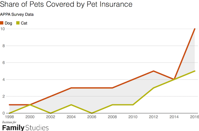
There is no autocorrelation for the model UAH = -0.33 + [1.5*log2(CO2)] + [0.12*ENSOlag4] + [0.20*AMOlag2] + [-5.0*AODvolcanic].
Anyway, autocorrelation is valid method of prediction, but I would not call it superstition. And is it any different conceptually than using any other statistical measure?
Oh i thought last week it was T = -0.25 + [1.4 * log2(CO2lag2)] + [0.10 * ENSOlag4] + [-4.0 * AODvolcanic] + [0.35 * UAHlag1].
What value is this considering i’d do just as well assuming next month will be the same as this month?
What does your exploratory data analysis mean? Is climate change related mostly to the relatively large coefficient determined for “AODvolcanic” ? Are your inputs correlated, or no? What have you left out, and why? What is the physical basis for choosing these specific parameters? What are your projections for 1 year from now, or 10 years from now?
JCM said: “Oh i thought last week it was T = -0.25 + [1.4 * log2(CO2lag2)] + [0.10 * ENSOlag4] + [-4.0 * AODvolcanic] + [0.35 * UAHlag1].”
I did. I have other models too.
JCM said: “What value is this considering I’d do just as well assuming next month will be the same as this month?”
I’m not sure that you can.
For T = UAHlag1 I get an RMSE of 0.126 C.
For T = [1.0*log2(CO2)] + [0.10*ENSOlag4] + [0.10*AMOlag2] + [-4.0 * AODvolcanic] I get an RMSE of 0.110 C.
JCM said: “What does your exploratory data analysis mean?”
It means we cannot eliminate CO2 as being a factor in modulating the UAH TLT anomaly value.
JCM said: “ Is climate change related mostly to the relatively large coefficient determined for “AODvolcanic” ?”
Not mostly, but partially. The coefficient is large because aerosol optical depths are small.
JCM said: “Are your inputs correlated, or no?”
Yes.
JCM said: “What have you left out, and why?”
A lot. I’ve left out dozens; maybe hundreds of parameters. I’ve left global circulation processing. The reason this is left out is because I don’t have the resources to include everything.
JCM said: “What is the physical basis for choosing these specific parameters?”
They have been shown to modulate the ingress and egress of energy in the atmosphere.
JCM said: “What are your projections for 1 year from now, or 10 years from now?”
I don’t have any. These models cannot predict 120 or even 12 months out. The autocorrelation model is limited to 1 month and the non-autocorrelation model is limited to 2 months.
Thanks. How are you handling the data uncertainties in your regression, and multicollinearity of the ‘independent’ variables?. It’s not ideal. Do you find the coefficients are extremely sensitive? If so, how certain do you feel about the actual effect of each variable?
I don’t do anything with the uncertainties of the inputs.
The coefficients aren’t that sensitive. They can be changed by several percentage points in some cases and not significantly change the final RMSE. I’m confident that the coefficients are optimal because I use recursive descent to optimize them.
What I’m not confident about is the model itself. I actually discovered that if I do 0.5 * model1 + 0.5 model2 I get an RMSE of 0.107 C where model1 is is the autocorrelation version and model2 is the CO2, ENSO, AMO, and volcanic version. The average of the two models has more skill, albeit only barely, than either of the two models alone. The ensemble is predicting 0.16 C for December 2022.
how are you accounting for AODvolcanic in advance?
The difference is that you have no theoretical foundation to predict a-priori the observed value. You can only infer based on ad-hoc selection of covariates. It is the same issue with the greenhouse gas effect hypothesis which relies ad-hoc on inputs of albedo, lapse rate, and a solar constant. It is why, to date, we are still missing a greenhouse effect theory. The unproven hypothesis must impose deliberate constraints on the atmospheric response to trace gas concentration. Scientists should be aiming to develop this theory, but instead there is tremendous focus on finding ways to reduce uncertainty of the data record. This focus is due to the fact that all which really exists is a correlation. It all hinges on this unproven hypothesis. The science is unable to establish the required quantitative relationship between GHG content and atmosphere to deduce temperature a-priori. So as of yet no theory exists.
JCM said: “how are you accounting for AODvolcanic in advance?”
Aerosol optical depths lag eruptions.
JCM said: “The difference is that you have no theoretical foundation to predict a-priori the observed value”
I have an entire body of evidence spanning nearly 200 years that links CO2, ENSO, AMO, volcanic activity, and prior atmospheric states (persistence) that says these factors play role in atmospheric temperatures. I then built a simple model based on this fact to test the claim I kept seeing here that the variability in UAH values necessarily precludes CO2 from having an impact on those values.
So would you mind posting your superstition model? I’d like to replicate it and see how much skill it really has.
Would you mind posting any model that you feel is scientific so that we can compare and contrast what you present with what I presented so that I can get a better understand of what you think is pro-scientific and anti-scientific?
I’m afraid I do not understand. spreadsheet games are tools for interpreting data. These tools can then be applied for developing scientific insights and theoretical frameworks. There is nothing anti-scientific about it, but rather failing to yet emerge from noticing a correlation. For it is unclear in your frameworks which are the dependent and independent variables, as you select ad-hoc convenient off-the-shelf data. You are still operating within the cum hoc ergo proctor hoc fallacy and appear to have failed to recognize this.
The dependent and independent variables in the model are obvious. CO2, ENSO, AMO, AOD, and UAHlag1 are independent. The UAH value itself is dependent. Remember, the measurement model in functional form is simply UAH = model(CO2, ENSO, AMO, AOD, UAHlag1).
I’m not making any statements about the definitive cause of UAH TLT anomaly changes. I’m only making statements about what UAH TLT will be 1 month in the future (a prediction by any reasonable definition) and why we should not eliminate either CO2, ENSO, AMO, and volcanic activity as contributing factors. The original intent was show how variations in UAH values are not inconsistent with the relatively steady and increasing CO2 values.
I could have made the model UAHnext = Σ[UAH_i, 1, N] / N. It’s skill would have been significantly less, but it would have provided a prediction nonetheless. In the same way we can predict the height of the next Swede. It might not be a “good” prediction according to some, but it will be a prediction nonetheless and I dare say in lieu of any other data points or information it will be the best anyone can do which is probably why no one is accepting Mosher’s challenge and instead claiming it isn’t even science.
i think it is perhaps a lost cause to engage further. this is absolute nonsense.
I think it’s nonsense that several people here seem to think it is offensive that one purpose of science is prediction. I also think it is nonsense that superstition can do a better job of predicting UAH values than what I believe is a legitimate science based approach. Yet I’m still willing to engage and hear people out. I don’t think you’re going to get that kind of willingness from everyone.
Function | Definition, Types, Examples, & Facts | Britannica
Note especially:
Like it or not, using coefficients to draw a curve is not a function. At best, it might be the derivative of a function which you could calculate through integration. I don’t see that happening since cyclical functions have trig components.
It is curve fitting where coefficients must change as the curve changes.
Dude, you can find the mean value is 6 1/2 feet. Yet the uncertainty is ±0.5 feet. It must be this unless you also specify that each person that was measured was exactly 6 feet or exactly 7 feet. No person was in between.
That is why the problem is ill posed. No uncertainty was quoted and no assumption about each person being only one or the other.
If the subjects varied in height from 5’6″ to 7’5″ then you have no way to make a prediction of what the next height might be.
If it is one or the other, then you have a coin flip. You still can’t predict the next value with anything resembling certainty.
bdgwx ==> Prediction is not the purpose of science. Discovery of new understanding is the purpose.
Science can be used to make predictions.
KP said: “Prediction is not the purpose of science”
I didn’t say it was the purpose of science. I said it is what science does. I’ll take it one step further though. Prediction is a purpose of science. Other purposes include, but may not be limited to, explanation and intervention. Anyway, a lot of people do science because of the predictions that can be made from doing it.
KP said: “Science can be used to make predictions.”
It sounds like you agreeing with me here.
“Prediction is a purpose of science.”
No.
As Kip wrote, understanding is the purpose of science. The only purpose. Deductive prediction, the outcome of understanding, is the test of understanding.
Kip isn’t agreeing with you. It appears, rather, that you’re confused about the fundamental distinction between inference and deduction. The former is what statistics does. The latter, science.
Pat Frank said: “As Kip wrote, understanding is the purpose of science. The only purpose.”
Let’s assume you really can’t use science to predict the height of a Swede. What do you recommend using?
You don’t even understand the issue do you? Two swedes, one 6′ and one 7′ is just like heads and tails. Can you predict accurately using “science” what the next flip will be?
Make predictions to test the science, that is, the statements about what was learned through the scientific process — unless it is such new science that there isn’t yet enough information to relate it to anything already known.
Science does not make extrapolations that are not based on evidence. Science is incremental. Climate science on the other hand is making doom and gloom predictions 80 years into the future based on what? Models that don’t match observations? Trends of data that are simple not fit for the use they are being used for?
How many people in the world are doomed to die because you think Armageddon is going to occur because of CO2? Think about it!
Your example is inference, bdgwx, not prediction.
I doubt he will listen.
My example contains elements of inference and prediction as does Mosher’s. The end goal, however, is to make a statement about an outcome that hasn’t happened yet; otherwise known as a prediction.
I’ll ask you the same thing here about the diagnoses and treatment protocols as I did above about the height of Swedes. If you don’t like the fact that one of the purposes of science is to make prediction then how would you predict the outcome for a specific person taking treatment protocol A or B before they have actually done it without using any element that could be reasonably associated with science?
“…and prediction…”
Not in any scientific sense.
All of medicine is based in Evolutionary Biology. Prediction of an individual outcome requires knowledge of the individual’s genome and metabolism. Such knowledge is typically not available.
Any such prediction would test the theory (level of knowledge).
Generally, however, your question misses the mark. It evidences misconceptions about science, namely you continue to conflate statistical inference with deductive prediction.
Ok, fine. I’ll accept that I cannot convince you that science can make a prediction about the outcomes of treatment protocols A and B or that it isn’t a purpose of science in general. What method, other than science, do you propose to make predictions regarding medical treatment protocols, the height of Swedes, or any other outcome in the world around us?
“I cannot convince you…”
You evidently cannot distinguish between statistical inference and physical prediction.
The outcomes of medical procedure A or B are invariably statistical. They do not predict the result in any given human. Hence, for example, the pages of tiny print possible side effects.
The rest of your comment is about statistical inference. Not science. Not prediction.
If determinism and a non-inference mandate is your standard for science then you probably didn’t consider the odds of me pulling the quantum mechanics card on you.
And exactly how many direct measurements are made on quantum objects?
How many indirect measurements? Funny how those indirect measurements have uncertainty such that we can’t determine quantum objects to a minus infinity resolution.
Quantum Mechanics is completely deterministic. The wave function evolves in strict conformance with the physical equations of the quantum state.
QM is a physical theory — it makes predictions. Inference has no place.
PF said: “Quantum Mechanics is completely deterministic.”
Oh? So now quantum mechanics is completely deterministic is it?
PF said: “QM is a physical theory — it makes predictions.”
I was told that making predictions is not science.
PF said: “Inference has no place”
Yeah, I know. You already told me that if you use statistical interference then you haven’t done science.
Here is a list of other preposterous claims in this subthread.
Prediction is not one of the purposes of science.
If you make a prediction you aren’t doing science.
If you use statistical inference you aren’t doing science.
Science mandates deterministic results.
Quantum Mechanics is completely deterministic.
My personal favorite…Superstition is at least as good as science.
I fully expect that if we let this conversation go on long enough someone will claim that if you are doing math you aren’t doing science.
And this all started because Mosher presented a simple challenge to predict the height of a Swede.
“take a set of data and uses it to make a prediction about the next data point” is mere inference.
Science deduces. Predictions come from a falsifiable physical theory.
Sorry dude, that is not what science does. Science takes a set of data and makes a hypothesis about what has occurred and how it may be defined mathematically. Science say here is what I did and how you can repeat my experiment.
Other folks may do the experiment such that results are more refined. Others may change things to see if the results are predictable using the hypothesis. Only when sufficient testing has been done can one say what the next data point MAY be. Doing that is extrapolating from current data and is subject to considerable doubt. The extrapolation may prove true, but it is a guess to begin with.
Right on, Jim.
Say they are extraterrestrials not Swedes and we had no preconception about how tall they are.
Already we have extremely useful information from this experiment. We know they are not 1 foot tall nor 50 foot tall.
In fact we can say with high confidence that their average is close to 6.5 feet, and the range of possible heights statistically unlikely to be much bigger than 1 foot either way from the mean.
No! The choice is 6′ or 7′, just like heads or tails. What is the average of tails as zero and heads as 1? Is it physical?
There was no uncertainty given in the problem, so 6.5′ is not an allowed value!
If you want to allow 6.5′ then you must allow an uncertainty of ±0.5′, so values from 5.5′ to 7.5′ can occur.
Again, this is a group of single readings each with an uncertainty of ±0.5. What is the Standard Deviation of your distribution?
I said that values from 5.5 to 7.5 feet can occur. The experiment does not disallow that possibility.
I suppose we need some additional information. Are the measurers recording to the nearest foot and that turns out to be 6′ or 7′ because all the sample of Swedes were between 5.5′ and 7.5′?
Or are all Swedes either 6′ exactly or 7′ exactly?
What if the two groups you measure have been pre-selected on height? That, to me seems to be what is being presented. In the real world, making two samples of 50 each would never give such measurements without determined biasing.
Actually, with a tape which is 7′ long, graduated in 1′ increments, you have only established the lower bound. Anything above 6’6″ will be recorded as 7′.
For all we know, half the aliens are 6′ +/- 6″, the other half range from 6’6″ to 12’6″
I don’t think trick questions tell us much about the issues under discussion.
No, but Mosh’s formulation was ill-posed. It would be less ambiguous with an 8′ tape measure.
We need the problem to be specified more closely.
However, I will say that with heights of a population, the expectation would be that it is a continuous distribution. All heights are permitted, not just 6′ and 7′ exactly.
Otherwise why use heights? If it were an either/or problem with only two possible outcomes, it would be better to use coin flips, not heights.
I therefore concluded that the experiment involved recording a continuous distribution of heights to the nearest whole foot.
Yeah, just saying that as specified we don’t really know the upper bound. If the tape measure was 8′ long and there were no 8′ aliens recorded, we could make the upper bound inferences, otherwise a recorded 7′ is just 7′ or taller.
Your question is nothing more than flipping a coin. You give no measurement error nor the uncertainty involved with each measurement.
Temperatures are not either/or. They are continuous physical time varying phenomena. Your question should be more akin to what is the true height of those you have measured. Is systematic error involved? what is the zero error involved?
Your question is ill posed and you don’t even know it.
For once you summed up neatly the correct use of the mean.
There is so much cross purposes and misunderstanding on these threads.
Here’s an average swede ?mode=crop&width=1423&height=711
We need more information about the experiment.
Are the measurers measuring to the nearest foot?
Or is it the case that all Swedes measured are either exactly 6 feet tall or exactly 7 feet tall ?
Two quotes seem relevant here.
Attributed to Rutherford:
‘If your experiment needs statistics, you ought to have done a better experiment.’
Miguel de Cervantes Saavedra:
‘At this point they came in sight of thirty to forty windmills that there are on plain, and as soon as Don Quixote saw them he said to his squire, “Fortune is arranging matters for us better than we could have shaped our desires ourselves, for look there, friend Sancho Panza, where thirty or more monstrous giants present themselves, all of whom I mean to engage in battle and slay, and with whose spoils we shall begin to make our fortunes; for this is righteous warfare, and it is God’s good service to sweep so evil a breed from off the face of the earth.” “What giants?” Said Sancho Panza.’
fah ==> Ah, Rutherford. I had an employer who demanded a dizzying array of stats (reports of sales, productivity of various areas, monies sent for varying things — literally dozens of them from each unit). But, in his favor, he absolutely forbade any analysis other than “Just look at the time series.” He did allow simple eye-balled trend lines.
IPCC CliSci sees dragons — us Pancho’s see windmills.
Bring back Don Quixote — with modern weapons!
Another fine demonstration that nothing can be allowed to impugn the veracity of the Holy Air Temperature Trends.
“There are lies, damned lies and statistics.” – Mark Twain
ScienceABC123 ==> In the spirit of uncertainty: “Mark Twain did include this saying in an installment of his autobiography which he published in 1907; however, he did not claim to be the originator; instead, Twain credited Benjamin Disraeli. Yet, there is no substantive evidence that Disraeli crafted this remark. He died in 1881, and the remark was attributed to him posthumously by 1895.”
There are more howevers…..
I can’t find the reference now, but Disraeli apparently came out with this line in a dispute with Charles Babbage.
Babbage was undoubtedly brilliant, but “difficult”
Nice essay Kip. I sent you an email with some info. Let me know if you don’t get it.
I hope some on here realize that you are not advocating the use of the CLT in climate temperature measurements.
The folks who need to justify it are those showing minute uncertainties and small, small values temperatures.
But they aren’t actually showing temperatures, are they. They are statistical numbers presented to the public (and the politicians) dressed in temperature robes.
Uncertainty does not mean ‘I don’t know’, it means ‘I cannot know’. This is a very uncomfortable concept for some to accept. For if we are not sure, it means anything is possible. Some have not quite wrapped their heads around this. ‘I am uncertain’ does not mean ‘I could be certain’. One cannot derive information about the unknowable with maths.
JCM ==> A subtle but important point. For a temperature measurement that has been rounded and recorded as 27 +/- 0.5°, the stated “absolute uncertainty” means both. We don’t know what the thermometer reading was before it was rounded and now, and in the future, we cannot know.
Those who argue this exhibit a phobia of the unknowable. Personally, I find the idea delightful. Like a warm fuzzy blanket on a cold winter day.
The charge that the parameters we are seeking are “unknowable” is certainly the all purpose excuse to do nada. “If I don’t have the perfect number straight from The Imaginary Guy In The Sky, then I can’t move my arms and legs”. FYI, it’s the antithesis of the “engineered answer”. I.e., the answer that’s cheap and practical enough to find to an accuracy and precision sufficient to act.
You highlight an important notion which drives the phobia of uncertainty – the desire to persuade. “to find” a method sufficient to elicit a desired action. This is motivated by belief. Rest assured, actions are possible even with imperfect or fuzzy knowledge.
“a method sufficient to elicit a desired action”
Is not why we seek engineered answers. We seek them to improve processes and/or solve problems. Yes, we engineers unabashedly “desire” this. That work has nada to do with “belief”. The prejudgments are those of the “unknowable” spouters.
how does one “engineer” data necessary to persuade from a non purpose built historical observation network?
“how does one “engineer” data”
You don’t. We engineers use that data appropriately to arrive at (AGAIN) the “engineered answer”. That’s the answer that’s good enough to act on. It need not come from above, which, effectively, is the WUWT requirement. Of course that is always couched in convenient banalities about how the “measurand is unknowable”, but it all ends up in the same, mulish, spot.
Are we talking about social engineering? i don’t follow. How does one engineer answers from old temperature readings?
Or on proxy data, do you find such illustrations credible? Or are such depictions motivated by factors outside the realm of science? To some, this raises red flags – that we may no longer be dealing in objective judgement and communication of what is known or knowable.
https://arxiv.org/abs/2212.04474
Your graph just tweaks one of my pet peeves. Labeling “anomalies” as TEMPERATURE. That is propaganda that attempts to tell and persuade people that TEMPERATURE has increased by 100%, 200%, or even 500% when it has done no such thing.
it is a lie. plain and simple.
What’s more, the ability to persuade is contingent on a relationship between science and society built on trust. This trust relationship must be held to the highest standard to maintain integrity. Scientists risk breaching trust by hiding or denying the existence of uncertainty.
Who wouldn’t agree?
No, no one I know is saying to do “nada”. Myself, I am saying that we are uncertain of two things, that Tmax temps are increasing dramatically, and that CO2 is the cause.
Ask yourself why we only see a Global Average Temperature. Why don’t we see a Global Average Maximum Temperature AND a Global Average Minimum Temperature? We have the numbers, what is the problem?
Why hasn’t climate science taken the minute data that is available and use integration techniques to find a daily “average” temperature that is infinitely more precise that using two readings per day?
Temperature is a physical, continuous, time varying phenomenon. Why is climate science not using time series analysis to evaluate temperature trends instead of simple regression to make predictions? I know, I know, models are being developed yet they are based on inadequate temperature profiles of land temperatures.
Instead of concentrating on CO2, why have there been no papers (that I have found) where careful placement of temperature sensors have been located around generators of UHI along with detailed analysis of its affects on total land temperatures?
Long post, but you need to evaluate more carefully just how serious climate science is about doing increasingly detailed studies using better techniques available with new technology.
Lack of change in science, is to many, an indication that climate science is not willing to do the work to prove their doomsday prognostications.
It’s silk purse out of sow’s ear, all the way down.
“Myself, I am saying that we are uncertain of two things, that Tmax temps are increasing dramatically…”.
Your view of the “uncertainty” of temp increase is from random and systemic data error. What you ignore is that, even the most extreme estimates of these errors merely thickens the error bars in any real evaluation of physically/statistically significant rime periods. They, in turn adds very little to the standard error of the resulting (another no no word in WUWT) trend.
“…and that CO2 is the cause.”
Not the sole cause. Who says that? What we know is that the increasing concentration of CO2 and other GHG’s is the only physically credible reason for the rate of increase in earthly temps. A rate not found before, outside of cataclysmic natural events. All other culprits floated here have nowhere near the forcing strength to produce such changes, no matter how wishfully widgeted together.
Again, AGW is the only “engineered answer”.
You’re delusional, blob, you’ve swallowed the watermelon nonsense hook, line, and sinker.
What is the optimum CO2 concentration level in Earth’s atmosphere? Shirley as an “engineer” you have this number sorted and close at hand.
And how much of your personal payday are you willing to donate for the Great Net Zero Project?
5%?
10%?
20%?
40%?
If real answers were to come out of all that work, there is always the chance that lamp posts beckon.
The numbers presented are intended to confuse the minds of the gullible, not to inform in any useful way.
Some winter days demand a heated blanket — but sigh, the wind isn’t blowing.
The “I cannot know” sounds a bit more like indeterminacy than uncertainty, although it depends on why “I cannot know”. In Quantum Mechanics, the “uncertainty” is not the inability to do a precise measurement of position, but more that a precise position does not exist.
conjecture. the Shrodinger’s cat paradox thought experiment was meant to illustrate possible problems with quantum theory. I think this is outside the scope of the discussion of historical temperature approximations, and judgement of uncertainty bounds.
John Christy’s new paper:
Anyone have access to a full copy of “Time Series Construction of Oregon and Washington Snowfall since 1890 and an Update of California Snowfall through 2020” by John R. Christy ?
https://doi.org/10.1175/JHM-D-21-0178.1
I’d love a .pdf.
I have a pdf, Kip. Email me at pfrank_eight_three_zero_AT_earthlink_dot_net and I’ll send it over.
Pat ==> Done.
Kip – sent. 🙂
Another interesting thing about dice, and kids, etc., is any actual result is a whole number. One can never actually roll the mean 3.5 nor have half a child.
I’d suggest in relation to measurement capability that early thermometers were a bit like that…not able to discern a value with precision less than 0.5C. I know my primary school wooden ruler was like that 0.5mm at best…the line markings were so thick.
macha ==> Early thermometers were know to be somewhat erratic as the size of the mercury column (diameter of the inside of the tube) was created by stretching a hot glass tube which did not produce a precisely even tube. To be a fair thermometer, they needed to be individually calibrated (marked in degrees) against some “standard thermometer”.
It would be interesting to list the the things that have impermissible values…..
“Erratic”? Sounds like a textbook source of normally distributed uncertainty to me. Is there any evidence of systemic error either way? If so, was it (the bad word) adjusted out in evaluations?
“Is there any evidence…”
Studied ignorance, given past conversations.
Common dude. Normally distributed? It is systematic error and statistics CAN NOT be used at this late date to remove the errors. They remain.
In addition, the glass used over time would flow causing the column to change and therefore more systematic error.
The best 19th century thermometers were individually scored while passing a small column of mercury up the capillary, so as to account for any variable width.
Some very long 19th C thermometers were good to ±0.05 C, but they were rare.
The usual meteorological thermometer was scored in 1 C or 1 F divisions and so could be read by eye to the nearest 0.25 C/F. But that is an ideal that was rarely met in the field.
A generally unrecognized problem is that neither mercury nor ethanol have a constant coefficient of thermal expansion, which means that errors creep in between the calibration points (usually 0 C and 100 C).
Pat ==> Yes, all very true. sadly ignored in CliSci today.
I surveyed the national weather station for the country of Dominican Republic for Anth0ny’s first Station data project. The National Chief Meteorologist gave us the tour…a Stevenson Screen, properly placed away from buildings, but in the middle of a corn field that was actively producing (so bare some of the year, corn six feet high other parts of the year). Next to the Stevenson Screen was a perfectly normal concrete block — about 8 x 12 x 8 inches. I asked about it.
“That’s for the shorter weathermen who take the daily readings, so they can be at the right level to read the thermometers….. but most of them are too proud and won’t use it, so our readings are a little high…a degree or so. ” [The meniscus problem].
I seem to remember that LIG thermometers are also affected by glass creep similar to how old window panes become thicker toward the bottoms.
You’re referring to Joule drift, KM. It’s a serious problem in pre-1900 LiG thermometers and one generally ignored in the field.
I plan to address this in a future submission.
Pat,
Lab thermometers were probably that accurate. The NWS still required field records to be rounded and recorded to the nearest degree. When these records are transcribed, there is no way to know what the true reading was, i.e., +/- 0.5 degree minimum.
NOAA’s ASOS user guide at:
aum-toc (weather.gov)
is the image I have attached. Not much, if any improvement.
Thanks, Jim. Very useful.
At age about 9 years, our class of post-war students, 60 of us under one teacher, all received a gift that influenced the rest of my life. It was a normal foot-long ruler marked in inches and eighths of an inch. This led me to work out the decimal numbers for each eighth as in 7/8 = 0.875) and so led to a math interest. The main benefit, though, came from the construction. There were little slabs of about ten different, polished woods from a selection of Australian trees, each labelled with species name. Great grounds for kindling an interest in botany, in art (beautiful patterns, how were they made/) and in propaganda (when there was little else to appreciate in a boring class, get interested in trees). Geoff S
http://www.geoffstuff.com/school.jpg