Guest Post by Willis Eschenbach [see update at end]
Over at the marvelous KNMI website, home of all kinds of climate data, they’re just finishing their transfer to a new server. I noticed that they’ve completed the migration of the Climate Model Intercomparison Project 6 (CMIP6) data to the new server, so I downloaded all of the model runs.
I thought I’d take a look at the future scenario that has the smallest increase in CO2 emissions. This is the “SSP126” scenario. KNMI has a total of 222 model runs using the SSP126 scenario. Figure 1 shows the raw model runs with the actual temperatures.

Figure 1. Raw results, 222 model runs, CMIP6 models, SSP126 scenario
So here, we have the first problem. The various models can’t even decide how warm the historical period was. Modeled 1850-1900 mean temperatures range all the way from twelve and a half degrees celsius up to fifteen and a half degrees celsius … hardly encouraging. I mean, given that the models can’t replicate the historical temperature, what chance do they have of projecting the future?
Next, I took an anomaly using the early period 1850-1880 as the anomaly baseline. That gives them all the same starting point, so I could see how they diverged over the 250-year period.

Figure 2. Anomalies, 222 model runs, CMIP6 models, SSP126 scenario
This brings up the second problem. As the density of the results on the right side of the graph shows, the models roughly divide into three groups. Why? Who knows. And by the time they’re out to the end of the period, they predict temperature increases from what is called the “pre-industrial” temperature ranging from 1.3°C up to 3.1°C … just which number are we supposed to believe?
Finally, the claim is that we can simply average the various models in the “ensemble” to find the real future temperature. So I compared the average of the 222 models to observations. I used an anomaly period of 1950-1980 so that the results wouldn’t be biased by differences or inaccuracies in the early data. And I used the Berkeley Earth and the HadCRUT surface temperature data. Figure 3 shows that result.

Figure 3. Global surface temperature observations from Berkeley Earth (red) and HadCRUT (blue), along with the average of the 222 climate models.
This brings us to the third and the biggest problem. In only a bit less than a quarter-century, the average of the models is already somewhere around 0.5°C to 0.7°C warmer than the observations … YIKES!
And they’re seriously claiming they can actually use these models to tell us what the surface temperatures will be in the year 2100?
I don’t think so …
I mean seriously, folks, these models are a joke. They are clearly not fit to base trillion-dollar public decisions on. They can’t even replicate the past, and they’re way wrong about the present. Why should anyone trust them about the future?
Here on our forested hillside, rain, beautiful rain, has come just after I finally finished pressure-washing all the walls, including the second story … timing is everything, the rain is rinsing it all down.
My warmest regards to all, and seriously, if you believe these Tinkertoy™ climate models are worth more than a bucket of bovine waste products, you really need to sit the climate debate out …
w.
Update: Rud Istvan, a valued commenter, pointed me to look at the INM climate model since it agrees well with the observations. When I took a look, I found an excellent example of the fact that past performance is no guarantee of future success …

Figure 4. Model runs from two versions of the INM-CM model.
As you can see, they both do an excellent job hindcasting the past, but give totally different versions of the future.
Further Reading: In researching this I came across an excellent open-access study entitled “Robustness of CMIP6 Historical Global Mean Temperature Simulations: Trends, Long-Term Persistence, Autocorrelation, and Distributional Shape“. It’s a very thorough in-depth examination of some of the many problems with the models. TL;DR version: very few of the model results are actually similar to real observational data.
In addition, there’s a good article in Science magazine entitled Earning The Public’s Trust on why people don’t trust science so much these days. Spoiler Alert: climate models get an honorable mention.
As Always: When you comment please quote the exact words that you are discussing. This avoids many of the misunderstandings that plague the intarwebs.
ah, well you see, in the future they’ll have better models!
for a good laugh try adding the UAH lower troposphere record 1979-2022
eyeballing the graph, the satellite-era warming trend of .16 per decade barely gets into the blue and is hilariously uncorrelated to the models
but don’t worry, any minute now half the population of the OECD will suddenly realize they’ve already wasted trillions of dollars and are planning to waste tens of trillions more
“for a good laugh try adding the UAH lower troposphere record 1979-2022”
They should combine Hansen 1999 and the UAH data and see if their models match that combination of data, representing 1880 to the present. This is the real temperature profile of the Earth. Unmodified, written, historical, regional surface temperature records from all over the world resemble the temperature profile of the U.S. regional chart, Hansen 1999, which shows it was just as warm in the Early Twentieth Century as it is today. No unprecedented warming. No need to worry about CO2. That’s what they show.
“I downloaded all of the model runs.”
I doubt it. I believe that only carefully selected model runs make it to CMIP6. Please prove me wrong, or maybe tell me who makes the selection.
Of course it’s not ALL the model runs. Lots of them ended up on the cutting room floor. I meant I downloaded all the listed CMIP6 model runs.
w.
One can only speculate the ratio of attempts to eventual useful product their models must perform … in the 100s or even the 1000s, yet still nothing useful comes from it.
An interesting point. Each model group selects what they chose to submit. That said, there are required submissions in the CMIP6 ‘experimental design’. So they freeze the parameters to best hindcast (a required submission) and then use that one for all the other submissions.
But wait. As I understand it, hindcasting is the same as comparing model output to past data records, but running the model in reverse. So is the data used the original data to the point of exit from the hindcast or is the data one or more of the thousands of adjusted data sets?
I dont think they run them in reverse per se.
They start up the model and let it run until it comes to an equilibrium because GCMs dont do climate change unless they’re explicitly forced. And by “forced” I mean adding forcings such as increasing CO2 levels.
Then they’ll introduce the “known” inputs from the historic period. eg CO2 increases, Aerosol changes which are not really “known” just chosen with post hoc justifications. The “date” will be the date of those prescribed, “known” observations as the model runs.
And they’re run through the past, present and out to the future (eg 2100) and the state of them is periodically sampled for later analysis. The future inputs are all configurable input guesses.
You do not run any sequential model ‘backwards’.
If it was warm today at 20C what was it yesterday and before?
What formula(s) would you use?,
Although many climate models including especially most of the CMIP6 ones have been working poorly, this is not because climate models can’t work. I see the problem being one of a groupthink of ignoring multidecadal oscillations. Most CMIP3, CMIP5 and CMIP6 models were selected and/or tuned for hindcasting, and mostly for hindcasting the 30 years before their hindcast-forecast transitions. During the last 30 years of the hindcasts of the CMIP3, CMIP5 and CMIP6 models, multidecadal oscillations were mostly on an upswing which is ignored in these models, so these models modeled warming caused by multidecadal upswing as being caused instead by positive feedbacks to warming from increase of greenhouse gases. Modeling the water vapor positive feedback as greater than it actually is causes the models to show a great tropical upper troposphere “hotspot of extra warming” while that hardly actually exists, as well as more warming overall after the hindcast-forecast transition dates of these models than has actually been happening.
I thought that models hope to be based on physics. What would be a physical base for multidecadal oscillations? These oscillations should be the output of models, not a built-in feature.
CG, the physics based claim was ALWAYS a canard. To be truly physics based, models have to compute stuff on a sub 4km grid cell (convection cells and Tstorms). Thanks to the CFL numerical solutions to partial differential equations constraint, they cannot—computationally intractable by 6-7 orders of magnitude. So they are forced to parameterize (references to previous posts explaining this above). And parameterization by definition isn’t physics. It’s guesstimates.
But they pay the rent, Rud. The politicians get what they pay for. Anybody that disagrees just doesn’t understand how the world works. The basics of human nature have been known for millennia.
GCMs predictions are based on “physics” in the same sense that an NPC in a Roblox game follows “physics”
not exactly tackling Navier-Stokes head on
as Feynman said, give me three parameters and I’ll give you an elephant, four and I’ll make it wag its tail
The parameterizations would work better if they’re done without ignoring what multidecadal oscillations did in the past while considering what sulfate aerosols, solar irradiance variations and greenhouse gas concentration change did in the past.
They couldn’t predict/project/hindcast/anycast tomorrow’s sunrise …
… the only things they have to calibrate themselves are the Hockey Stick and horribly adjusted temperature data – supposedly correlated/causated with CO2 data
So by time there’s no definitive or quantitative connection between CO2 and temperature (which there never can be) and that they’ve got the source of the CO2 wrong….
….there aren’t words to describe the wrongness
The various models can’t even decide how warm the historical period was.
_____________________________________________________________
From my file of quotes factoids and smart remarks:
Mark Steyn famously said: How are we supposed to have confidence in what
the temperature will be in 2100 when we don’t know it WILL be in 1950!!
Funny, I was just reading something on the movie Back to the Future.
“It turns out director Robert Zemeckis’ fantasy of the future failed to match up to reality. Not only are we deprived of such fanciful gadgets (hover boards and self tying shoelaces) and a Jaws 19 sequel, in this version of 2015 we apparently still read newspapers and have fax machines in every room. Fax machines! No internet. No Twitter. No insufferable influencers.”
Are science fiction stories set in 2022 more dystopian than real 2022? – ABC Everyday https://www.abc.net.au/everyday/what-did-science-fiction-get-right-about-2022/100882010
The future is not the past extrapolated.
There are an infinite number of possible futures. That’s why predicting it is a fools game.
People who claim to be able to predict the future are never seen placing bets at racetracks. That should tell you all you need to know.
He got the Cubs World Series win wrong by only one year, though.
(Their manager, Joe Maddon, was actually shooting for the 2015 win mentioned in the first sequel, for that very purpose!)
Hmmm… The difference in thermal emission (with emissivity at 0.95) at 12.5C is 358.6 W/m2. At 15.5C it is 373.9C. That’s a difference of over 15 W/m2.
But both models are trying to evaluate the effect of a change of less than 2 W/m2 (so far) from increased CO2!
Definitely a major problem …
w.
Very good.
Are the models improving over time (I sure hope so)?
If they are, and if the latest ones diverge ~0.5C from observations over just 25 years, just how bad were the old ones?
Ed Lorenz’ 1963 paper “Deterministic Nonperiodic Flow” says no. The only thing that has improved is the number and amounts of government grants funding computer playtime for academics, who always insist they need more.
As regards the IPCC, do get up climateaudit.org and take a look at Steve McIntyre’s exposure of another disgraceful fraud- the AR6 Summary frontispiece Hockey Stick. Fake. Why do we pay any attention to this self-important puffed up incompetent organization? And don’t forget the two books by Donna Laframboise which authoritavely catalogue multiple dishonesties
As I posted earlier, its the only game in town. Just keep hammering at their lies and the whole edifice will eventually collapse.
Even more crazy than the BS of climate models is the fact that renewable energy has been accepted as the answer. When one says well they are so variable the advocates just say they will be firmed with energy storage. The variability of wind and solar is such that that is not a viable solution. I have the data for this in the Australian context and find as Europe has recently experienced the extent of wind droughts. If you do the sums a 100 MW wind station which has no wind for 30 hours 831 megawatt hours to firm it. That is just not achievable on scale. The advocates also do not seem to be concerned that despite the large amount of work that has been done to reduce emissions it is not detectable in the atmospheric record.
“Even more crazy than the BS of climate models is the fact that renewable energy has been accepted as the answer.”
That is even more crazy.
There are a lot of delusional people running around the world. There are a lot of people taking advantage of those delusional people, too.
“I mean seriously, folks, these models are a joke.”
Great post and I really like your analysis!
If I understood correctly you picked a model ensemble with an unrealistic low CO2 scenario, correct? (If so the discrepancies to the real world are even worse for more realistic scenarios)
Last not least while of course I understand what you are saying, there is really nothing funny at all about this.
Until climate modelers use unadjusted data for benchmarking their models are going to run hot. I wonder if they even know that the data they are using for training the models has an artificially induced correlation with CO2 through the adjustment process. I would like to see what happens if they use the UAH data for training. My guess is that CO2 sensitivity would drop dramatically.
Subtract the mean of the models from the individual model runs and plot the residuals.
If they are like CMIP5 models the residuals will unstructured random noise. See my graph on Andy May’s recent post.
This is because the only information creating structure in the model outputs are the input forcing curves, which are common to all the models. This is the prior for the climate forward modelling. Without it, the models do nothing.
Except add noise.
Here is the graph I mentioned. This is for the 39 core models in CMIP5. I have subtracted the model mean to give the residuals for the 39 models. They are unstructured random noise. I suspect if WE does the same for the models in this post, the residuals will also be unstructured random noise.
Climate models are forward models. They only do what they are told to do by the input priors. Plus they add random noise. The spread of the models represents the lack of understanding of the physics to compute the temperature of the earth from first principles. That spread is greater than the entire C20th warming.
So when you average the models you filter the random part out (stack it out) and end up with just the low frequency. Which can be closely reconstructed simply by linear regression of the input priors – as WE has pointed out in a post at WUWT before.
As far as I can tell, climate models don’t add anything that isn’t already in the priors.
I have wondered what is the source of all the random variation.
Numerical instability?
Pseudo-stochastic parameters?
Epsilon-like round off errors and truncation?
Weird non-linear threshold decisions?
Who knows?
Bizarre random walks?
A modest proposal: Quit paying for all the models with results between +1 and -1; the 6 or 7 remaining, extreme models could then be used as inputs to all the senseless arguments about ECS and CAGW.
Using the SSP126 scenario highlights the poor agreement on the present temperature (a clear fail for consensus science) but reality, in terms of CO2, is closer to SSP585.
Even if Net Zero becomes the global mantra, it will take a massive amount of carbon to build all the energy extractors. In fact, trying to get to Net Zero increases carbon requirement because the low intensity, intermittent energy extractors and associated storage consume more energy than they can produce.
“This brings us to the third and the biggest problem. In only a bit less than a quarter-century, the average of the models is already somewhere around 0.5°C to 0.7°C warmer than the observations”
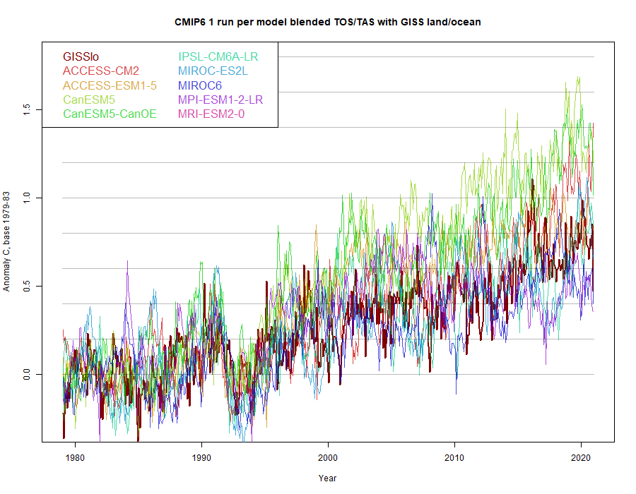
The problem is that this comparison is between the observed land/ocean and the modelled TAS. The first uses SST (sea temperatures) for the ocean component, and the second models air temperature throughout. It is just an observed fact that SST is warming less rapidly that air temperature.
This is true in the models too. They list a variable TOS, which is the equivalent of SST. Unfortunately, KNMI takes a while to post this variable. But it is available, and it agrees well with observed SST.
The appropriate way to compare, as in Cowtan et al 2015, is to blend TOS for ocean and TAS for land. This emulates the HADCRUT calculation. If you do, as I did here, the results agree much better (GISS is the dark curve):
ps this is over all scenarios, not just SSP126.
And, still, the GISS looks nothing like the models after the tuning period. Mash some hot models after the tuning period with some more realistic ones and they might look like the adjusted GISS crap. None of this proves CAGW. Nick is a sophisticated shill.
And Tom Karl used Night Marine Air (NMA) temperatures to adjust SST numbers. Jaysus, Nick, you can’t keep up with the changing dogma.
No, GISS looks very like the models to present, especially if you take out the outlier Canadian model.
Nick, you know damned good and well that the UN IPCC CliSciFi models are a scientific disaster yet you deny the obvious. Please show that, beyond the tuning period, that CMIP models reflect the variations of temperature and rainfall, much less those in the cryosphere. Post 2000 deviations are obvious.
You ignore the fact that Tom Karl used the Night Marine Air Temperatures (NMAT) to adjust SSTs. Subsequent to 2015, NMAT has deviated significantly from SSTs. WTF?
And if you squint real hard, touch your nose with the left index finger, while standing on your right foot, the models will tell you anything you want them to.
What do you people have against actual science?
“GISS looks very like the models to present,”
Its adjusted/manipulated/fabricated to be that way !
And they still miss.
Thanks, Nick. Around which period are the anomalies taken? And why did you start in 1980?
Next, I’m not clear why this should make a difference. The air temperature over the ocean tracks the ocean temperature very closely. Their differences are rarely more than a degree C, and are relatively stable in each location. See my post “TAO Sea and Air Temperature Differences“. That’s why the observational datasets (HadCRUT, Berkeley Earth etc.) are using SSTs as a proxy for air temperature.
This is even more relevant when we consider that we are interested in temperature increases, and when SST increases, TAS increases. Again, this is why they’re used in global observational temperature reconstructions, which consider anomalies rather than raw data.
Best regards,
w.
“Around which period are the anomalies taken? And why did you start in 1980?”
The anomaly base period is 1979-83. I used that, and post-1980, because I was comparing with the results of Roy Spencer, who chose those times.
“Next, I’m not clear why this should make a difference”
Well, indeed they are close, which is the basis for letting the better-measured SST stand in for SAT. But the relevant question here is whether they are different in the models, because if so, TOS for sea is clearly the right comparison with land/ocean indices. And the fact that blending makes a difference, as indicated, clearly says that this is so. I can’t easily locate a direct comparison of SST and TAS over ocean, but the linked paper of Cowtan et al shows the same effect of blending as I get:
Thanks, Nick. Using your base anomaly 1979-1983, by the end of the period, the observations are still a half degree below the average of your models.
So even with your measurements, the models are running hot.
Also, yes, I see that the air-ocean difference increases IN THE MODELS. But:
• In the quarter-century of the deviation shown in Figure 3, the air-ocean difference only changes trivially.
• I simply can’t imagine a physical reason why the modeled difference would change so much over time.
• Once again, we see a huge spread in the modeled results, with the air-sea difference going from a single lonely model showing ~ -0.5°C to the max difference of 0.25°C. I sure wouldn’t buy a used car if they told me “it has between 50,000 and 250,000 miles on the odometer” …
• This graph implies that there is a shift around the year 1975 from the ocean warming the air above it, to the air warming the ocean … please explain in simple terms how this massive shift might occur.
Seems to me you need to dial up your skepticism about the model results … as Alfred Korzybski sagely remarked, “The map is not the territory”.
My best to you,
w.
Willis,
Thanks. I was also saddened to hear of the death of Geert, whose work with CMIP especially I greatly appreciated. I don’t know if it is connected, but I found that it is not currently the most up to date with CMIP6. There is a site here which I last used about a year ago which seems to have a larger collection of results, including TOS.
Thanks for the link, Nick, I’ll take a look at that site. Sure wish the CMIP6 folks would put together an easily-accessible site to download ALL of the various model outputs.
Regards,
w.
Meaningless computer games.. Nothing more.
Ahh Nick. I have been posting this on and off for years in response to your ‘model’ posts and you have never answered.
I will try again, though I suspect there will be silence again.
“The Models are wrong. This is a fact not an opinion and it is a fact that can be shown.
Of course you cannot falsify them yet by just checking their forecasts against the real world as not enough time has passed to be definite. Also you cannot run an experiment with the Earth to falsify them.
However, there is another way to disprove any hypothesis. All you need to do is show that it produces an impossible result.
So what would be an impossible result for an accurate and correct model?
Well, what does a climate model output? It outputs a climate signal quantified by the Earth’s global temperature. This output is compared and graphed to past actual temperature data and is then taken forward to predict the future.
All the current climate models do very well on the hind cast against data. Remarkably so really, over the 20th century as the temperature data shows rises and falls so do the models track it with little variation except for the shortest periods. Is that good?…….. NO!
You see the models average out a lot of the natural variation factors, mainly ENSO. The designers original argument for this is that it makes the model simpler (true) and that anyway natural variation was so small it did not affect the main signal significantly. (false)
Now it is accepted that natural variation is strong enough to mask the true signal and for quite long periods, way longer than a decade.
So now both sceptics and warmists agree that natural variation (mainly ENSO) can completely alter the underlying modelled climate signal.
So we can see that the models and the temperature records are outputting different signals. One, a climate signal plus averaged variation and the other, the climate signal plus actual variation. It is now accepted that actual variation can cause the models to drift well away from reality for quite lengthy periods (see the long ‘pause’ at the start of this century). Therefore the fact that the models are currently drifting away from reality does not prove they are wrong. Indeed it is a behaviour that only an accurate model would display in anything other than neutral variation. It doesn’t prove it is correct but it certainly doesn’t prove it is incorrect
So what would be an impossible result for an accurate and correct model to output. Well clearly that would be a signal that does closely match the actual temperature data over the short to medium term. An apple doesn’t equal an orange no matter how you cut it. Only in the long run would the signals align. In the short to medium term an accurate model must run either hot or cold
So, given that ENSO has been doing its thing over the 20th century, the fact that on the back cast run the models track the temperature record very closely in all its up and down movements proves that these models are in fact false. That is an impossible result for an accurate model.
In their hubris, the warmists, when fiddling with their free parameters to make a great fit with the historical data, overlooked that they were trying to fit an apple to an orange! Or perhaps they didn’t think anyone would take much notice of them if they couldn’t even match the past.”
“Well, what does a climate model output? It outputs a climate signal quantified by the Earth’s global temperature. This output is compared and graphed to past actual temperature data and is then taken forward to predict the future.”
I think you have a poor understanding of models. They produce a great deal more than Earth’s average temperature, and the last sentence is totally wrong.
“You see the models average out a lot of the natural variation factors, mainly ENSO.”
Just not true. The models do ENSO. They aren’t synchronised, with each other or Earth, so it washes out in any kind of average, but each model has similar ENSO behaviour to Earth.
“historical data”
The historical data has been modified to fit the climate models(and vice versa), and is properly described as “adjusted” data.
There is a very big difference between the two.
The historical data shows we have nothing to worry about from CO2, because it is no warmer now than in the recent past even though there is more CO2 in the air now than then.
The adjusted data shows we are living in the hottest times in 1,000 years.
Here’s a visual, the U.S. surface temperature chart (Hansen 1999) along side a bogus, bastardized Hockey Stick chart. The U.S. chart shows CO2 is not causing unprecedented warming, and the bogus Hockey Stick shows just the opposite.
The historical temperature data was written down by people who did not have a human-caused climate change bias; who never heard of human-caused climate change.
The adjusted data, created in a computer, was formulated by people who DO have a human-caused climate change bias.
Is it any wonder the climate models are so far off? The Alarmists are living in a make-believe world of their own creation, and it doesn’t correspond with the real world.
The alarmists want us to live in that fantasy world, too. They want us scared and compliant. They think we are stupid.
Would anyone reading this site buy a car, boat, airplane, computer, computer model, etc. with as large a relative discrepancy of stated expected specs and actually delivered performance? Why are the politicians buying this Bovine excrement? I would have been fired if the computer programs I wrote were this bad. And the NRC would have shut down the plant and forced new models and safety analyses be performed, along with a hefty fine.
“Why are the politicians buying this Bovine excrement?”
Because it suits their purposes. Or, they are too ignorant and/or cowardly to go against the alarmist narrative.
Of course the models are a joke. Anyone who builds and uses models knows that relying on them for predictions of a non-deterministic system with so many variables, such as climate, is total and utter nonsense. As Willis says they can’t even model the past.
How anyone claiming to be a scientist can possibly believe the models are remotely accurate is a total and utter fool. I guess that would be all climate scientists, then.
I’m not sure that “fool” describes anyone that makes a lucrative career on misstating facts.
Frauds, is a better description. At least for some of them. I’m sure there are a few dupes thrown in there somewhere.
But the main players are frauds. They know better. They’ve seen all the data all the rest of us have seen (the historical temperature data). There is no unprecedented warming and they know it, yet they pretend there is.
<i>KNMI has a total of 222 model runs using the SSP126 scenario.</i>
This is the first puzzler since KNMI only has 144 SSP126 runs. Based on the caption it appears the ensemble here has been built from an unstructured web folder rather than the actual KNMI SSP126 ensemble. Based on the numbers I think there is a duplication of the already large number of CanESM5 runs, such that this single model (out of 30+ in CMIP6) produced 100 of the 222 runs used here. Importantly this model has the highest climate sensitivity of all models in CMIP6.
<i> the models roughly divide into three groups. Why? Who knows.</i>
See above for a big part of the reason. 45% of the runs come from a single model.
<i>Finally, the claim is that we can simply average the various models in the “ensemble” to find the real future temperature.</i>
Nobody has made that claim. In fact, with regards CMIP6, numerous mainstream climate scientists have clearly stated a belief that the CMIP6 ensemble mean produces too much warming, based on a number of models having higher climate sensitivity than the IPCC-assessed very likely range, as well as the rate of warming since the 1970s. Indeed the AR6 Summary for policymakers projections use observational constraints on the CMIP6 ensemble, for example indicating a best estimate of 1.8C (range 1.3-2.4C) for SSP126, versus 2.5C for the ad-hoc ensemble shown here.
<i>And I used the Berkeley Earth and the HadCRUT surface temperature data.<i>
This appears to be using HadCRUT4. The current version is HadCRUT5.
<i>In only a bit less than a quarter-century, the average of the models is already somewhere around 0.5°C to 0.7°C</i>
This is basically a function of the ad-hoc ensemble used here being massively over-weighted by the highest sensitivity models. Much better to use the one run per model ensemble mean at KNMI. This produces 2100 warming of 2C, with the current anomaly from 1950-1980 being about 0.1C above Berkeley/HadCRUT. In a historical difference plot between model mean and obs the current discrepancy is within normal variation.
c126names
[1] “ACCESS-CM2_ssp126_000” “ACCESS-CM2_ssp126_001”
[3] “ACCESS-CM2_ssp126_002” “ACCESS-ESM1-5_ssp126_000”
[5] “ACCESS-ESM1-5_ssp126_001” “ACCESS-ESM1-5_ssp126_002”
[7] “AWI-CM-1-1-MR_ssp126_000” “BCC-CSM2-MR_ssp126_000”
[9] “CAMS-CSM1-0_ssp126_000” “CAMS-CSM1-0_ssp126_001”
[11] “CanESM5_ssp126_000” “CanESM5_ssp126_001”
[13] “CanESM5_ssp126_002” “CanESM5_ssp126_003”
[15] “CanESM5_ssp126_004” “CanESM5_ssp126_005”
[17] “CanESM5_ssp126_006” “CanESM5_ssp126_007”
[19] “CanESM5_ssp126_008” “CanESM5_ssp126_009”
[21] “CanESM5_ssp126_010” “CanESM5_ssp126_011”
[23] “CanESM5_ssp126_012” “CanESM5_ssp126_013”
[25] “CanESM5_ssp126_014” “CanESM5_ssp126_015”
[27] “CanESM5_ssp126_016” “CanESM5_ssp126_017”
[29] “CanESM5_ssp126_018” “CanESM5_ssp126_019”
[31] “CanESM5_ssp126_020” “CanESM5_ssp126_021”
[33] “CanESM5_ssp126_022” “CanESM5_ssp126_023”
[35] “CanESM5_ssp126_024” “CanESM5_ssp126_025”
[37] “CanESM5_ssp126_026” “CanESM5_ssp126_027”
[39] “CanESM5_ssp126_028” “CanESM5_ssp126_029”
[41] “CanESM5_ssp126_030” “CanESM5_ssp126_031”
[43] “CanESM5_ssp126_032” “CanESM5_ssp126_033”
[45] “CanESM5_ssp126_034” “CanESM5_ssp126_035”
[47] “CanESM5_ssp126_036” “CanESM5_ssp126_037”
[49] “CanESM5_ssp126_038” “CanESM5_ssp126_039”
[51] “CanESM5_ssp126_040” “CanESM5_ssp126_041”
[53] “CanESM5_ssp126_042” “CanESM5_ssp126_043”
[55] “CanESM5_ssp126_044” “CanESM5_ssp126_045”
[57] “CanESM5_ssp126_046” “CanESM5_ssp126_047”
[59] “CanESM5_ssp126_048” “CanESM5_ssp126_049”
[61] “CanESM5-CanOE_ssp126_000” “CanESM5-CanOE_ssp126_001”
[63] “CanESM5-CanOE_ssp126_002” “CanESM5-CanOE-p2_ssp126_000”
[65] “CanESM5-CanOE-p2_ssp126_001” “CanESM5-CanOE-p2_ssp126_002”
[67] “CanESM5-p1_ssp126_000” “CanESM5-p1_ssp126_001”
[69] “CanESM5-p1_ssp126_002” “CanESM5-p1_ssp126_003”
[71] “CanESM5-p1_ssp126_004” “CanESM5-p1_ssp126_005”
[73] “CanESM5-p1_ssp126_006” “CanESM5-p1_ssp126_007”
[75] “CanESM5-p1_ssp126_008” “CanESM5-p1_ssp126_009”
[77] “CanESM5-p1_ssp126_010” “CanESM5-p1_ssp126_011”
[79] “CanESM5-p1_ssp126_012” “CanESM5-p1_ssp126_013”
[81] “CanESM5-p1_ssp126_014” “CanESM5-p1_ssp126_015”
[83] “CanESM5-p1_ssp126_016” “CanESM5-p1_ssp126_017”
[85] “CanESM5-p1_ssp126_018” “CanESM5-p1_ssp126_019”
[87] “CanESM5-p1_ssp126_020” “CanESM5-p1_ssp126_021”
[89] “CanESM5-p1_ssp126_022” “CanESM5-p1_ssp126_023”
[91] “CanESM5-p1_ssp126_024” “CanESM5-p2_ssp126_000”
[93] “CanESM5-p2_ssp126_001” “CanESM5-p2_ssp126_002”
[95] “CanESM5-p2_ssp126_003” “CanESM5-p2_ssp126_004”
[97] “CanESM5-p2_ssp126_005” “CanESM5-p2_ssp126_006”
[99] “CanESM5-p2_ssp126_007” “CanESM5-p2_ssp126_008”
[101] “CanESM5-p2_ssp126_009” “CanESM5-p2_ssp126_010”
[103] “CanESM5-p2_ssp126_011” “CanESM5-p2_ssp126_012”
[105] “CanESM5-p2_ssp126_013” “CanESM5-p2_ssp126_014”
[107] “CanESM5-p2_ssp126_015” “CanESM5-p2_ssp126_016”
[109] “CanESM5-p2_ssp126_017” “CanESM5-p2_ssp126_018”
[111] “CanESM5-p2_ssp126_019” “CanESM5-p2_ssp126_020”
[113] “CanESM5-p2_ssp126_021” “CanESM5-p2_ssp126_022”
[115] “CanESM5-p2_ssp126_023” “CanESM5-p2_ssp126_024”
[117] “CESM2_ssp126_000” “CESM2_ssp126_001”
[119] “CESM2_ssp126_002” “CESM2_ssp126_003”
[121] “CESM2_ssp126_004” “CESM2-WACCM_ssp126_000”
[123] “CIESM_ssp126_000” “CNRM-CM6-1_ssp126_000”
[125] “CNRM-CM6-1_ssp126_001” “CNRM-CM6-1_ssp126_002”
[127] “CNRM-CM6-1_ssp126_003” “CNRM-CM6-1_ssp126_004”
[129] “CNRM-CM6-1_ssp126_005” “CNRM-CM6-1-f2_ssp126_000”
[131] “CNRM-CM6-1-f2_ssp126_001” “CNRM-CM6-1-f2_ssp126_002”
[133] “CNRM-CM6-1-f2_ssp126_003” “CNRM-CM6-1-f2_ssp126_004”
[135] “CNRM-CM6-1-f2_ssp126_005” “CNRM-CM6-1-HR_ssp126_000”
[137] “CNRM-CM6-1-HR-f2_ssp126_000” “CNRM-ESM2-1_ssp126_000”
[139] “CNRM-ESM2-1_ssp126_001” “CNRM-ESM2-1_ssp126_002”
[141] “CNRM-ESM2-1_ssp126_003” “CNRM-ESM2-1_ssp126_004”
[143] “CNRM-ESM2-1-f2_ssp126_000” “CNRM-ESM2-1-f2_ssp126_001”
[145] “CNRM-ESM2-1-f2_ssp126_002” “CNRM-ESM2-1-f2_ssp126_003”
[147] “CNRM-ESM2-1-f2_ssp126_004” “EC-Earth3_ssp126_000”
[149] “EC-Earth3_ssp126_001” “EC-Earth3_ssp126_002”
[151] “EC-Earth3_ssp126_003” “EC-Earth3_ssp126_004”
[153] “EC-Earth3_ssp126_005” “EC-Earth3_ssp126_006”
[155] “EC-Earth3-Veg_ssp126_000” “EC-Earth3-Veg_ssp126_001”
[157] “EC-Earth3-Veg_ssp126_002” “EC-Earth3-Veg_ssp126_003”
[159] “EC-Earth3-Veg_ssp126_004” “FGOALS-f3-L_ssp126_000”
[161] “FGOALS-g3_ssp126_000” “FIO-ESM-2-0_ssp126_000”
[163] “FIO-ESM-2-0_ssp126_001” “FIO-ESM-2-0_ssp126_002”
[165] “GFDL-ESM4_ssp126_000” “GISS-E2-1-G_ssp126_000”
[167] “GISS-E2-1-G-p3_ssp126_000” “HadGEM3-GC31-LL_ssp126_000”
[169] “HadGEM3-GC31-LL-f3_ssp126_000” “HadGEM3-GC31-MM_ssp126_000”
[171] “HadGEM3-GC31-MM-f3_ssp126_000” “INM-CM4-8_ssp126_000”
[173] “INM-CM5-0_ssp126_000” “IPSL-CM6A-LR_ssp126_000”
[175] “IPSL-CM6A-LR_ssp126_001” “IPSL-CM6A-LR_ssp126_002”
[177] “IPSL-CM6A-LR_ssp126_003” “IPSL-CM6A-LR_ssp126_004”
[179] “IPSL-CM6A-LR_ssp126_005” “KACE-1-0-G_ssp126_000”
[181] “KACE-1-0-G_ssp126_001” “KACE-1-0-G_ssp126_002”
[183] “MCM-UA-1-0_ssp126_000” “MCM-UA-1-0-f2_ssp126_000”
[185] “MIROC-ES2L_ssp126_000” “MIROC-ES2L_ssp126_001”
[187] “MIROC-ES2L_ssp126_002” “MIROC-ES2L-f2_ssp126_000”
[189] “MIROC-ES2L-f2_ssp126_001” “MIROC-ES2L-f2_ssp126_002”
[191] “MIROC6_ssp126_000” “MIROC6_ssp126_001”
[193] “MIROC6_ssp126_002” “MPI-ESM1-2-HR_ssp126_000”
[195] “MPI-ESM1-2-HR_ssp126_001” “MPI-ESM1-2-LR_ssp126_000”
[197] “MPI-ESM1-2-LR_ssp126_001” “MPI-ESM1-2-LR_ssp126_002”
[199] “MPI-ESM1-2-LR_ssp126_003” “MPI-ESM1-2-LR_ssp126_004”
[201] “MPI-ESM1-2-LR_ssp126_005” “MPI-ESM1-2-LR_ssp126_006”
[203] “MPI-ESM1-2-LR_ssp126_007” “MPI-ESM1-2-LR_ssp126_008”
[205] “MPI-ESM1-2-LR_ssp126_009” “MRI-ESM2-0_ssp126_000”
[207] “NESM3_ssp126_000” “NESM3_ssp126_001”
[209] “NorESM2-LM_ssp126_000” “NorESM2-MM_ssp126_000”
[211] “UKESM1-0-LL_ssp126_000” “UKESM1-0-LL_ssp126_001”
[213] “UKESM1-0-LL_ssp126_002” “UKESM1-0-LL_ssp126_003”
[215] “UKESM1-0-LL_ssp126_004” “UKESM1-0-LL_ssp126_005”
[217] “UKESM1-0-LL-f2_ssp126_000” “UKESM1-0-LL-f2_ssp126_001”
[219] “UKESM1-0-LL-f2_ssp126_002” “UKESM1-0-LL-f2_ssp126_003”
[221] “UKESM1-0-LL-f2_ssp126_004” “UKESM1-0-LL-f2_ssp126_005”
You are correct that some models are over-represented. But what I wanted was to show all the runs on file. Why? Because I don’t trust the “one run per model”, because I have no idea which run to choose. There are no a priori calculations that would tell us which of the large number of runs of any given model we should choose … nor is there any justification for the idea that the average of a model’s runs will be more accurate than simply picking a run at random …
I also wanted to show the foolishness of the whole idea of an “ensemble” because it depends quite sensitively on just which runs of just which models make up the “ensemble”
My point remains untouched. There is a HUGE difference between not only individual models, but also individual runs of the same model, and even between different versions of the same model, for example …
Perhaps you can educate us just which of those two runs we should believe?
w.
I saw the same differences among model runs past 2020 or so when I looked at the SSP scenarios, too, Willis. Some runs of the scenario turned down, others did not.
I figured the difference arose because some models followed only the Meinshausen forcings. In the SSP126 scenario, CO2 forcing turns down in mid-century. Models following that forcing only, will project a mid-century down-turn in air temperature.
The models projecting increasing temperature past mid-century may include the contribution of ocean heat after the CO2 forcing transient turns off.
The INM-CM4-8 and INM-CM5-0 model runs may be different in that way.
My best to you.
Thanks as always, Pat. The idea of averaging over models is crazy with that kind of stuff going on.
w.
Agreed, Willis.
You found the same problem with CMIP6 models that Jeffrey Kiehl found with the CMIP3 versions.
They were all able to closely reproduce the historical air temperature trend, but they varied in ECS by factors of 2-3. Their projected trends zoomed off in very divergent trajectories. Just as you found for the CMIP6 models.
Kiehl was struck by the dichotomy. All the same pasts, but different futures.
He realized that the offsetting errors that tuned models to reproduce past climate, went on to produce very different futures.
Still, despite the uncertainty hidden in the models, Kiehl genuflected to the accepted paradigm. I.e., “It is important to note that in spite of the threefold uncertainty in aerosol forcing, all of the models do predict a warming of the climate system over the later part of the 20th century.“
I weep at the CliSciFi groupthink and misdirection based in ideology that is reflected in the Kiehl quote. He ignores the fact that all the models were tuned to “… the later part of the 20th century.” and didn’t “predict” crap.
Thanks, Pat, true. I wrote about this in Dr. Kiehl’s Paradox.
Best to you and yours,
w.
Thanks for the listing, that confirms what I thought. There are “only” 50 CanESM5 CMIP6 SSP126 runs in existence but you have 100 there. I think at one point KNMI had all 50 in one ensemble, but then changed to split them in two parts. The directory you used contains both ensemble setups so your selection duplicates all the CanESM5 runs.
Just pick one at random. Pretty sure the KNMI ensemble just uses the first ensemble member for each model. Here’s a quick experiment: setup 100 monte-carlo one-run-per-model ensembles, each time selecting a random run from each model. I would guess there will be barely any difference between the 100 ensembles.
It’s really not a question of accuracy of the runs. It’s about properly representing the ensemble by weighting members appropriately so the results aren’t dominated by a single model, as in your setup.
Of course results depend on what models make up the ensemble, but that doesn’t at all demonstrate anything about the usefulness of an ensemble. The purpose of an ensemble is simply to represent uncertainty because a single model can’t tell us much about that. No-one is suggesting that any given ensemble is perfect, but it’s better than not having an ensemble at all. Also, the sensitivity to which members make up the ensemble is dependent on properly weighting, which is why attention should be paid to doing that.
Not sure why this is a point? Demonstrating the difference between models is the purpose of the ensemble.
That’s a curiosity so I’ve taken a look. The first clue is that the historical periods line up exactly, which is impossible if they are from different model versions. Turns out that the black line is actually the SSP245 run of INM-CM4.8 – it presumably got mislabeled by somebody at some point. Go to the KNMI front-end and plot INM-CM4.8 SSP126 and SSP245. You’ll get the same plot you just posted.
Are you suggesting some models are more right than others? In that case, there must be some incompetent modellers.
I know for a fact that all models bear no relevance to Earth’s climate system. They can never function with any skill until they can replicate convective instability of tropical oceans that limit ocean surface temperature to annual maximum of 30C. Once that is done, any notion of catastrophic global warmings is eliminated. And all this nonsense goes into the waste bin where it belongs.
Note though that AR6 poster child model mean comparison to temps Figure in the SPM uses HadCRUT4.
So HadCRUT4 seems to be the appropriate comparison.
It is meaningless to average temperature over different models. There is no central limit theorem for models. Another problem is that each model makes it own assumptions about aerosols. But only one or possibly none of them has the right amount. This means that averages are taken over a lot of models that make wrong assumptions about the concentration of aerosols. This more looks like the fruits of the poisoned tree.
I believe that was one of the first lessons in reasoning we learned … ‘two wrongs can’t make a right’.
If every time you do something in a particular way you get a bad result, stop doing it and reevaluate the method.
You are correct.
The reason they do it (probably unintentionally) is because it filters out the noise and reveals the common input to the models – the prior forcings.
But because the climate model mean can be generated accurately using simple linear regression of the prior forcings this tells us the models are redundant. The match to obs. temps arises because the priors already match the temp profile, once scaled into the same units.
Odd, the temperature doesn’t square with the University of Alabama data. Why is that?
Unlike the Politicians I would be reluctant to bet the farm on unvalidated climate models.
That’s what the politicians are doing. They are not reluctant at all.
We have climate change group-think in our political class and it is leading us down the road to ruin.
Let’s hope we can turn this around in Nov. 2022, and Nov. 2024.
We have to remove these insane radical Democrats from power over our lives. One year of this insanity ought to be enough for anyone with any sense, to see we are heading down the wrong road fast.
The radical Democrats do not have the answer for anything. Everything they do is detrimental to the United States and its people.
I think this post combined with aspects of the model dissection WE did recently would be timeless
When I’ve confronted people regarding models I’ve used that post to demonstrate how ridiculous they really are.
Meaning, the graphs above show the future limits of model projections but are those limits simply shoulder rails in the code to keep the results from running off into true insanity?
Well done
The answer is that these models are dyslexic; 3.1 should read 1.3. Or, perhaps 1.3 should read 3.1. Or something.
What is interesting when you look back at various ‘models’ throughout history is the amount of times they utterly didn’t work.
What is the big shock should not be ‘the models are wrong’ but ‘the models were wrong and we somehow didn’t completely destroy ourselves by following them’.
Climate Change models – yeah, enough said within this forum.
COVID 19 predictions – yup. Remember the hundreds of thousands who were absolutely going to die within the first months?
We can also look back deeper into the historical record. Prior to WW2 there was a strong theory that ‘The Bomber Would Always Get Through’. Now to be fair in practice stopping a bombing raid was extremely difficult but sustaining a bombing offensive in the face of constant resistance was also extremely difficult. Point was it was believed that come a war there was no way to prevent the bombing of UK cities. Hence if they were going to be bombed, they needed to work out how many would die. The models (that M Word again) worked out that if one ton of bombs could destroy a set area and kill a set amount of people, then 10 tons of bombs would do 10 times as much… cause… linear. Basically everyone would die so the mass evacuation of children was brought into play. Sure I am certain that some children had a grand adventure, but the record also shows that for many being forcefully removed from their parents and homes and forced to live with complete strangers was utter hell. Models.
I guess on the plus side without these predictions less money would have been spent on the air defence of Great Britain, but the underlining point was the models were wrong.
Same war while I am on the topic, since physically shooting in combat conditions at enemy warships was expensive during times of peace nearly all naval powers used ‘wargames’ (or Models) to attempt to predict the best way to fight enemy ships in various situations. All sorts of wonderful systems based on average hit rates and shell effects vs armour and damage ability were brought into play and the research departments tested theories and wrote suggested tactics and everyone was happy. Cause the Models told them they should be.
Come the war and we had the Battle of the River Plate. German ‘Pocket Battleship’ vs three RN cruisers. Now the models had studied this as the use of Pocket Battleships as commerce raiders was something everyone was expecting. The models said the two Leander class cruisers with their 6 inch guns should engage a Pocket Battleship at long range using rapid fire and smoother the German ship with hits. These would overwhelm the enemy in about 30 minutes and VCs all around. Jolly Good Show.
So that is what they did.
Spoiler? It didn’t work.
The Graf Spee took only a few hits from the 6 inch guns despite the two cruisers firing off nearly all their ammunition. They kept firing because that is what the models told them would work.
Since the Germans weren’t taking damage from the two 6 inch cruisers they concentrated on the HMS Exeter and worked her over badly to the extent the Germans could/should have overwhelmed and sunk her. The other two RN ships eventually realised they had done next to nothing for over an hour – much longer than the models had predicted – and changed tactics.
Short summary – the Germans went into a neutral port, discovered damage to their galley would prevent them from feeding their crew on any extended voyage back to Germany and, rather than going out in a pointless blaze of glory against the reinforced British, scuttled in a blaze of smoke and the British, realising they had very nearly snatched defeat from the jaws of victory wrote up the entire thing as a brave battle against a MASSIVELY superior enemy in the bravest traditions of the Royal Navy, and not ‘our tactics were wrong, we barely even hit the enemy and utterly wasted our advantage in numbers and weight of fire.’
Why? THE MODELS WERE WRONG.
Face it, the only useful model is made of plastic and one of the landing wheels knocked off when your mother attempted to dust it.