By Andy May
In the Great Climate Change Debate between Professor David Karoly and Professor Will Happer, Glenn Tamblyn was called upon to finish the consensus side of the debate after Karoly backed out. The details are described in my latest book. The debate contained an illuminating exchange of opinions on satellite versus surface temperature measurements. This is Glenn Tamblyn’s opinion:
“Stitching together raw data from multiple satellites is very complex. Thus, the satellite datasets are much less accurate than the surface temperature datasets.
Professor Happer’s stronger emphasis on satellite temperature measurements does not agree with the experts on the subject.”
(Tamblyn, 2021b, pp. 7-8)
Satellites measure microwave radiation emitted from oxygen atoms in the atmosphere to estimate the “brightness” temperature, which can then be converted to an actual atmospheric temperature. No correlation to any other measurements is required. The measured brightness is compared to the brightness temperature of deep space (-455°F) and a target of known temperature within the satellite to compute the actual temperature in the atmosphere.[1]
Due to interference and clouds, this technique does not work close to the surface, so satellite atmospheric temperatures cannot be directly compared to surface measurements. The satellite measurements are best for measuring air temperatures in the mid-troposphere and the lower stratosphere.
The Hadley Centre has estimated that their best current estimate of global monthly average SST accuracy (sea surface temperature average uncertainty from 2000 to 2021) is about ±0.033°C and David Karoly supplied an estimate of ±0.1°C. This is a bit less accurate than the accuracy Roy Spencer and John Christy estimate for their satellite measurements of ±0.011°C for a monthly average.[1]
Given these peer-reviewed analyses, we can comfortably assume that the satellite data is at least as accurate as the surface data, if not more accurate. Besides, the satellite data covers a larger volume of the atmosphere, and it uniformly covers more of the globe than the surface data.
Tamblyn seems to think that because the data used to create the satellite record is from multiple satellites, this necessarily means the satellite temperature record is less accurate. This is incorrect, the satellites are merged with an accurate procedure described by John Christy.[2]
We also need to remember that the surface measurements are made in a zone with great volatility and a large diurnal variation. The satellites measure higher in the atmosphere, in a more stable environment, and are better suited to estimating climate change, as opposed to surface weather changes.

In Figure 1, the UAH satellite lower troposphere temperature record (light blue) is centered at about 10,000 feet.[2] It is compared to the Hadley Centre sea surface temperatures (HadSST4, in gray) and the land and ocean surface temperature dataset (HadCRUT5, in orange).
Happer, clearly states that the satellites are measuring a different temperature and have consistent, nearly global coverage. Ground measurements, on the other hand, are sparse, irregularly spaced, and made with many different devices.[3]
In Figure 1 we can see the HadSST and the UAH satellite lower troposphere warming trends are identical at 0.14°C/decade. The major difference is that the El Niños and La Niñas are more extreme in the lower troposphere than on the surface. Two prominent El Niños are visible in 1998 and 2016. Prominent La Niñas have the reverse relationship to the El Niños as seen in 2008 and 2011.
The HadCRUT5 dataset is well below the other two in the beginning of the period and above at the end. It has a warming rate of 0.19°C/decade. This 36% increase in warming rate is entirely due to adding land-measured surface temperatures to the SSTs, even though land is less than 30% of Earth’s surface.
Figure 1 leads us to three important conclusions. First, the El Niño years support the idea that a warmer surface will lead to more evaporation, which carries heat from the ocean surface to the lower troposphere; the same process that carries heat from an athlete’s skin into the atmosphere. As the evaporated water condenses to droplets, usually in clouds, it releases the heat of evaporation into the surrounding air. The lower troposphere UAH temperature, plotted in Figure 1, is most sensitive to temperatures around 10,000 feet, but it includes some emissions below 6,500 feet, which is a common altitude of lower clouds.
Second, since the overall rate of HadSST warming is about the same as the UAH lower troposphere warming, it suggests that the extra warming in the HadCRUT5 land plus ocean dataset is suspect.
Third, if HadCRUT5 is correct, it means the surface is warming faster than the lower and middle troposphere. If this is true, the IPCC Reports and models suggest that the warming is not due to greenhouse gases.[4] It could be that additional warming in the troposphere, above 6,500 feet, is due to El Niños and not due to GHGs (greenhouse gases). It is hard to accept that the data plotted in Figure 1 is both accurate and consistent with the idea that greenhouse gases are causing surface warming. For a further discussion of the relationship between GHGs and the ratio of surface to middle troposphere warming see my previous post.
In summary, both common methods of determining the global average temperature, satellite, and surface, are probably accurate to within a tenth of a degree, as suggested by Karoly. Both methods show the world is warming, but currently the HadCRUT5 surface warming estimate of 0.19°C/decade is significantly higher than the satellite lower troposphere and SST estimates of 0.14°C/decade. The excess surface warming is entirely due to land measurements or adjustments to them. The adjustments made to the CRUTEM5 land surface temperature measurements and the similar Global Historical Climatology Network (GHCN) are significant and controversial as explained by Peter O’Neill and an impressive list of coauthors.[5] To be clear, O’Neill, et al. evaluated the GHCN data and not CRUTEM5, but the adjustments to each of these datasets are similar and they both have the same weaknesses. The justification for the 36% increase in warming rate between the ocean and the land plus ocean records is not clear and probably indicates a problem with the CRUTEM5 land temperature record, the greenhouse gas warming hypothesis, or both.
Download the bibliography here.
This post was originally published at the CO2 Coalition.
-
(Spencer & Christy, 1990) ↑
-
(Christy, Spencer, & Braswell, 2000) ↑
-
(Kennedy, Rayner, Atkinson, & Killick, 2019) and (Karl, Williams, Young, & Wendland, 1986) ↑
-
(IPCC, 2021, pp. Figure 3-10, page 3-162) and (IPCC, 2013, pp. Figure 10.8, page 892). The dependence of the higher tropospheric warming trend on the CO2 greenhouse effect is most easily seen in the 2013 AR5 report since they present natural warming in blue and greenhouse warming in green in their figure. ↑
-
(O’Neill, et al., 2022) ↑
Satellites at least have no infill or missing stations problem. As the satellites agree with weather balloons, I would regard them as more reliable than surface stations, which do have a UHI issue.
Also, when you have 100% coverage of the planet, homogenization can’t be used to distort the data.
Not exactly 100% coverage. I think UAH is 85N-85S and RSS 80N-80S (back before it was “adjusted”.
Satellites do give the best coverage we’ve had.
There are also polar orbiters (NOAA-N) that can fill in the N and S polar regions, not necessarily with the u-wave measurements, but with other data that can be correlated to the u-wave measurements and produce similar temperature proxies.
The area above 85ºN and below 85ºS is a bit less than 1M.km² each
The area of the planet is about 510 M.km²
That means that the UAH data misses only about 0.4% of the planet.
1M km sq. About one Waddam?
🙂 Lols
Satellite data is not 100% coverage all day&night. They have a large % coverage after each cycle but how long does that take? They try to combine data from multiple satellites (multiple sources, multiple different design/aged sensors).
See figure 7.4
https://www.sciencedirect.com/topics/earth-and-planetary-sciences/metop
From Wiki..
“Satellite temperature measurements are inferences of the temperature of the atmosphere at various altitudes as well as sea and land surface temperatures obtained from radiometric measurements by satellites.
Satellites do not measure temperature directly. They measure radiances in various wavelength bands, which must then be mathematically inverted to obtain indirect inferences of temperature. The resulting temperature profiles depend on details of the methods that are used to obtain temperatures from radiances. As a result, different groups that have analyzed the satellite data have produced differing temperature datasets.
The satellite time series is not homogeneous. It is constructed from a series of satellites with similar but not identical sensors. The sensors also deteriorate over time, and corrections are necessary for orbital drift and decay. Particularly large differences between reconstructed temperature series occur at the few times when there is little temporal overlap between successive satellites, making intercalibration difficult.”
https://en.wikipedia.org/wiki/Satellite_temperature_measurements
All important points to remember, the UAH LT data are a convolution of the sensor responsivity with the 0-10km altitude air temperature that decrease exponentially from the surface.
Temperature is never measured directly. A common thermometer measures the expansion or contraction of mercury or alcohol as a proxy for temperature. You can’t measure the kinetic energy of a gazillion molecules.
That looks like an interesting publication. Unfortunately it is paywalled and I can’t find a free copy. I was able to find another interesting paper by some of the same authors using the GOES-R satellites as well.
Inferring missing links and other purposes.
And…the best surface station network (US) covers only 6% of the earth’s surface area and is compromised by many stations falling out of siting specifications due to land use changes.
Many regions have only very sparse coverage.
UAH only has the 9504 of the10368 grid cells filled with values, but they label their global average temperature as being from 90S to 90N which means they are effectively filling in the 864 unfilled cells with the average of the 9504 filled cells to get that full sphere average.
The only datasets that have true full sphere coverage are reanalysis like ERA5. The ERA5 warming is +0.19 C/decade which matches HadCRUT. Note that unlike UAH which uses a trivial global weighted infilling strategy HadCRUT uses a local weighted gaussian regression strategy.
bgdwx
Let me add that as opposed to UAH 6.0, UAH5.6 had a 100 % coverage as well.
This is visible only when processing the two grids for comparison purposes.
Download e.g. ‘tltmonacg_5.6′ or ‘tltmonamg.1979_5.6‘ from
https://www.nsstc.uah.edu/data/msu/t2lt/
and you will see that the topmost and bottommost three latitude bands contain valuable data.
Interesting. I wasn’t aware that v5 had 100% coverage. Interesting indeed!
It is better to hide what you can’t accurately observe.
And, as another commenter wrote, that’s no more than 0.4 % of the Globe, and even less if you take the latitude weighting into account.
” As the satellites agree with weather balloons… ”
Firstly, you very certainly don’t mean ‘satellites’, but rather UAH’s processing of NOAA satellite data.
Moreover, you claim sounds to me a bit strange, because ‘satellites’ in fact agree best with those weather balloon (radiosonde) processing methods which were derived from… satellite data.
To be convinced, you just need to consider the weather balloon subset named RATPAC (RATPAC-A for yearly, RATPAC-B for monthly data).
RATPAC is a tiny subset (85 units) of the about 1500 weather balloons (radiosondes) managed by NOAA within the IGRA data set.
The data provided by these 85 units is highly homogenized, according to techniques (RAOBCORE, RICH) developed about 15 years ago at Vienna U (Austria).
Here you see a comparison I made years ago, of the homogenized RATPAC-B data with
– the original data out of the IGRA data set;
– the average of the entire IGRA data set.
RATPAC-B shows considerably lower trends and higher homogeneity than the IGRA set out of which it was originally selected.
*
Feel free also to have a look at an interesting publication:
Satellite and VIZ–Radiosonde Intercomparisons for Diagnosis of Nonclimatic Influences
John R. Christy and William B. Norris (2006)
https://journals.ametsoc.org/view/journals/atot/23/9/jtech1937_1.xml
There you see how 31 radiaosondes peu à peu miraculously fit satellite data.
*
IGRA radiosonde data starts in 1958, and has data for 13 different atmospheric pressure levels, from surface up to 30 hPa (i.e. about 21 km altitude).
The 700 hPa level was selected for the graph below, because it is nearest to the 10,000 ft mentioned above in Andy May’s head post; moreover, the average absolute temperature of UAH measurements is around -9 C, what gives, when considering a lapse rate of 6.5 °C / km in the LT, about 3.7 km, corresponding to 640 hPa.
Here is the graph:
In blue, you have RATPAC-B at 700 hPa; in red, UAH Globe land.
{ The reason not to choose UAH Global (land+ocean) is that most radiosondes (70 % in RATPAC) are located on land, the rest being on islands. }
Trends for 1979-2022, in °C / decade:
*
But not quite surprisingly when you are familiar with UAH analyses like that made by Richard E. Swanson, the best polynomial fit calculated in a spreadsheet out of RATPAC-B data is obtained when you select the 300 hPa level.
That means however an altitude of about 9 km, where you hardly could find the temperatures measured by UAH for the LT.
Sources
IGRA
https://www1.ncdc.noaa.gov/pub/data/igra/
RATPAC-B
ftp://ftp.ncdc.noaa.gov/pub/data/ratpac/ratpac-b/
Bindidon, Thanks, very helpful addition to the discussion.
Andy May, thanks in turn for the convenient reply.
In fact I wanted to post a longer comment showing more aspects of the radiosondes data.
But I lacked the time to do, and post right here what I had intended to add.
*
You wrote above
” Both methods show the world is warming, but currently the HadCRUT5 surface warming estimate of 0.19°C/decade is significantly higher than the satellite lower troposphere and SST estimates of 0.14°C/decade.
The excess surface warming is entirely due to land measurements or adjustments to them. “
And in a previous document, you wrote:
” It is possible that the urban heat island effect, combined with the UK Hadley Centre homogenization algorithm has contaminated the land-only CRUTEM5 record and distorted it. “
” Frankly, it suggests there is a problem with CRUTEM5. Figure 3 suggests the problem is getting worse in recent years, not better. “
If that was the case: how then do you interpret this comparison of CRUTEM5 with the surface level of the same RATPAC-B radiosonde data?
Trends for 1979-2022, in °C / decade:
CRUTEM5’s trend for 1958-now (0.22 C / decade) is somewhat higher than that of the radiosonde data (0.22 C / decade).
This is only due to the lower temperatures before 1990, because while CRUTEM5’s trend for 2000-2022 keeps at 0.28, that of the radiosonde data is 0.34 °C / decade.
So your claim about “problems with CRUTEM5” is quite questionable when we compare Hadley’s land surface series with RATPAC-B.
Please don’t tell me that after agreeing to a match of RATPAC-B at 700 hPa with UAH6.0 LT, you would suddenly dispute a match of the same RATPAC-B at surface with a surface time series like CRUTEM5.
*
Furthermore, if you compare the trend of a global surface series (0.19 C/decade) to the trend of a lower tropospheric series (0.14 C/decade) and claim the former is too high just because the latter’s trend is as low as it is that of a sea surface series (0.14 C/decade), then that is not plausible either.
Because as a comparison of UAH6.0 with its previous revision UAH5.6 suggests, we could perfectly interpret the agreement of the UAH global data with a sea surface series as an ocean cooling bias in UAH.
*
I’m quite convinced that a mix of natural causes like heat transfer from the SH to the NH via the Thermohaline circolation, together with anthropogenic causes (UHI, GHE increase) will over the long term provide for a much better explanation than these permanent guesses about biases in land surface measurements.
” CRUTEM5’s trend for 1958-now (0.22 C / decade) is somewhat higher than that of the radiosonde data (0.22 C / decade). ”
should read
” CRUTEM5’s trend for 1958-now (0.22 C / decade) is somewhat higher than that of the radiosonde data (0.19 C / decade). “
In Climate Consensus World, “experts on the subject” should be taken to mean “those who agree with me”
Hi Andy.
Great piece. Conclusion is the same as mine. It ain’t the CO2 who did it.
https://breadonthewater.co.za/2022/03/08/who-or-what-turned-up-the-heat/
It would be great if you could let me know if you agree with my essay. Best wishes.
Henry,
Most of the essay is fine, but a quick read found two things I do not agree with:
Lots of people disagree with this. The ACRIM TSI record shows solar output increasing to around 2000-2005, then beginning a decline. See here:
IPCC Politics and Solar Variability – Andy May Petrophysicist
I do not think volcanic activity has caused any warming in recent times. It can though. The Siberian Traps volcanism (Permian) had an effect for a very long time. The NAIP volcanism of the PETM (Tertiary) also had a long-term effect. More minor eruptions, like Mt. Pinatubo lasted several years at most. Some info here: The Paleocene-Eocene Thermal Maximum or PETM – Andy May Petrophysicist
I will have more in the next few weeks.
Wrote about short term effects of VEI 5-6 (not thousands of years long flood basalt eruptions like the Siberian Traps), just ‘ordinary’ stuff like Pinatubo, in essay Blowing Smoke in eponymous ebook. The short term cooling effect of stratospheric aerosols lasts at most 2-3 years. Presented all the physical science ‘proofs’.
Thanks Andy.
I have strong proof from a statistical analysis of daily data from 54 weather stations balanced on latitude that Tmax started to go down from 1994-1995.
I think I will try to add this into the essay.
However, as we now know, earth kept warming up. So the extra heat is or has come from somewhere else.
The only way to explain the results in Table 2 is extra volcanic activity in the arctic ocean and arctic region. I have given a number of volcanoes that have erupted there.
I have added that graphic in my essay.
it seems most people do not understand that most volcanoes are on the bottom of the oceans. If they erupt, you do not get to see much, especially if is is very deep. It is just the heat that goes into the ocean. Most gasses like CO2 , sulphur and chlorine will be dissolved in the water before you even see it because of the high temperature.
When you conaider heat capacity it is nonsense to calculate average temperature of air and water using a simple average. This violates the conservation if energy.
(T1+T2)/2 = avg(T)
only works when the two objects are the same material and the same mass.
Perhaps this: Intensive and extensive properties – Wikipedia
Let me make it even simpler. If you put a thermometer into two liquids in two containers of different size, each containing a liquid of different heat capacity, and each thermometer reads the same, then the average temperature of the two containers is, guess what?
Nevertheless, a man can become woman of the year. 🙂
Snip snip.
Ouch!
… and Bob’s your Auntie
This confounds thermal mass and temperature concerning ‘heat’. Higher thermal mass contains more ‘heat’ (using statistical mechanics definition) but can be as same temp. Change Delta T requires different delta heat, granted. But the resultant expressed as delta T (not delta heat) should be additive.
Lay translation—to previous comment to the last Andy May post. INM CM5 has higher ocean thermal inertia, one of two main reasons it more closely resembles observations. The reason is exactly the distinction between heat and temp mediated by thermal mass.
By mathematical definition, it is indeed correct to state that the average temperature = (T1 +T2)/2, just as it would be correct to state that the average velocity for a fly and a supersonic transport would be (Vfly+Vsst)/2.
See Tom.1’s reference to the difference between intensive and extensive properties.
I believe you are thinking that temperature is a direct measurement of the heat (sensible thermal energy) content of a liquid . . . nothing could be further from the truth.
To link temperature to energy, one has to consider not only heat capacity, which you mentioned, but also total mass and whether on not the temperature measurement is being made at the exact point of phase change in the material (e.g., for water, the freezing/thawing or boiling/condensation points).
ERA5 uses hourly grids processed on ~12 timesteps. The global average temperature computed from those grids is similar to HadCRUT’s (Tmin+Tmax)/2 strategy.
We know that many surface stations have physical problems with siting and maintenance, and not only in the US. The satellites don’t.
Plus, UAH is able to discern whether there is a tropical troposphere hotspot as modeled by all BUT INM. (There isn’t one.) See my comment to Andy’s last post concerning INMCM5.
So naturally, the alarmists prefer the poorer land surface record that shows more warming, as this excellent post shows.
NOAA has consistently demonstrated that they can make temperature whatever they desire.
h/t Tony Heller
Here is a graph from Gavin Schmidt’s attempt to explain away the CMIP6 models divergence from observations AND how he would prefer to show the model outputs instead of
John Christy’s most recent spaghetti graph.
On realclimate.org [where this image came from] he discussed the graph.
Note that 1) Gavin has arbitrarily removed all the models that he thinks are running too hot,
then does the average [there are 2 colors of models] & then 2) uses surface temps rather than satellite data so it looks like the models are more accurate.
I believe this doctored graph is the one Simon uses all the time.
It’s also convenient how the area between the warmest and coolest models are shaded in hiding all of the individual models. Hiding the fact that all of the models except the Russian model run hotter than even the surface data.
Nobody hides data better than a climate scientist.
There is no scientific justification for averaging the results of various climate models. Basically, the practice is scientific misconduct.
Supposedly the averaging is done to try and get rid of “noise” leaving only the anthropogenic signal. But how does a model produce “noise” in the first place?
That “scientific misconduct” you speak of is used to provide more objective skill (as scored by the anomaly correlation coefficient) in forecasts of the 500 mb heights (and other fields) for operational weather forecasts provided by ensemble models like the GEFS and EPS.
No matter what the errors time will show the trend.
Looking at satellite data for say sea level has the errors larger than the yearly trend as such ask me in two decades what has happened.
Using the errors to help persuade, is the fraud.
These temperature constructs are getting more & more confusing.
My local weather report now posts what the current temperature “feels like”.
I’m moved to ask –
“is that when a cloud bank passes overhead?”
OR
“is that when I’m standing directly in the sunshine, or under a tree?”
OR
“is that just after I’ve had a haircut, a shave, and trimmed my eyebrows, nose hair and ear hair?”
OR
“when having a pee by the forest trail, I didn’t realize it was that cold that day!“
With enough averaging, a record that has no trend will be transformed into one that has a trend. The real (unsmoothed) record of global temperature is in the former category. It is just one long so-called “pause”, which is interrupted by occasional steps during El Ninos. Without the El Ninos, even averaging wouldn’t produce a trend.
https://rclutz.com/2022/03/11/still-no-global-warming-cool-february-land-and-sea/
El Ninos aren’t caused by CO2.
I agree with your words Phil, but I find your graph highly dubious. The HadCRUT4 40’s and 50’s seem rather low.
I was wondering if anyone else saw this. Congrats.
If the steps up are driven by El Nino’s then the first question to ask is what drives the El Nino’s. I am highly doubtful that it is CO2 growth in the atmosphere. The second question to ask is that since that which goes up usually comes down at some point, when can we expect to see the stairsteps down? I’m guessing this is part of a cyclical process. One that the models simply don’t incorporate.
Andy’s is a good defense of the satellite data. The only thing I would add is that the lack of amplified warming in the deep layer temperatures from the satellite versus surface temperature could be due to stronger negative IR feedback than climate models have. Specifically, weak positive or zero water vapor feedback and high cloud feedback (i.e. Lindzens infrared iris) would cause what is being seen, and the forcing could still be increasing CO2. There is no way to know for sure.
Rubbish – ocean surface temperature is limited to 30C over any annual cycle. The sky goes dark day and night over open oceans if the temperature reaches 31C and the surface temperature then regulates back to 30C.
Heat loss is regulated by sea ice such that the water below the ice never gets colder than -1.8C.
These two powerful thermostatic limits regulate earth’s energy balance.
Orbital precession is the dominant driver of the observed climate trends. Atmospheric CO2 is irrelevant to any direct climate impact on the energy balance.
The Nino 34 region has cooled over the last 40 years:
http://bmcnoldy.rsmas.miami.edu/tropics/oni/ONI_NINO34_1854-2021.txt
No climate model shows a cooling trend for the last 40 years over the Nino34 region.
RW, I appreciate your contributions—to a point, The AGW/Climate Change claims have to do mainly with the atmosphere over the land where we live. (Because nothing else is sufficiently scary.) So all your ocean points are at least secondary. No matter if true. And I have yet to see you convincingly couple them here.
Clearly you have not understood the fundamentals of Earth’s energy balance.
Globally, land masses always absorbs heat from the oceans. That is the nature of net precipitation; latent heat absorbed in oceans and some released over land to form precipitation thereby warming the land by reducing the rate of cooling. Without oceans, Earth would be cooler.
The net radiation balance over land is always negative and usually positive over oceans. Oceans absorb heat and give it to the atmosphere over land:
https://wattsupwiththat.com/2021/11/14/global-water-cycle/
Easy for anyone with an ounce of knowledge and a curious mind to verify.
No climate model has predicted the observed reduction in freshwater runoff from land over the past 50 years.
https://www.bafg.de/GRDC/EN/03_dtprdcts/31_FWFLX/freshflux_node.html
https://www.pnas.org/doi/10.1073/pnas.1003292107
The lag in warming is supposed to be due to ocean thermal inertia. All climate models rely on the claimed energy imbalance warming the oceans. The CSIRO model shows the ocean surface in the western Pacific reaching 40C by 2300 – per attached. That is just crazy nonsense.
Globally, land is always cooler than the oceans so there can be no catastrophic warming without oceans playing along with that unphysical requirement.
I agree Roy. But I sure wish the possible problems I’ve highlighted in the last two posts with the land-temperature records (both GHCN and CRUTEM) were looked into. Looking at the discrepancies straight up and simply, it sure looks like the data is bad or GHGs are not important, at least if you believe the models (I don’t).
You are correct, there are other possible explanations for the discrepancies, but are the IPCC looking into them? As far as I can see they only consider GHGs, volcanic eruptions, and aerosols, everything else is held constant. Seems over simplistic, but that is what I see.
Andy May, you mention “The adjustments made to the CRUTEM5 land surface temperature measurements and the similar Global Historical Climatology Network (GHCN) are significant and controversial…”
Here is an illustration of the effect of adjustments, looking at July Tavg data for years 1895-2021. No claim is being made here concerning the validity of adjustments. I am just showing the bulk results for one month for the contiguous U.S.
The USHCN is a subset of GHCN covering the contiguous U.S. There is a list of 1,218 stations for which monthly data is available here at this link as final values after pairwise homogeneity adjustment (FLs.52j), time-of-observation adjustment (tob) and as raw values.
https://www.ncei.noaa.gov/pub/data/ushcn/v2.5/
The readme.txt file explains the file formats and coding. There is a DMFLAG description:
E = The value is estimated using values from surrounding stations because a monthly value could not be computed from daily data; or, the pairwise homogenization algorithm removed the value because of too many apparent inhomogeneities occuring close together in time.
So I analyzed the July data in the FLs.52j file for tavg to separate “E-only” flagged data and not-E-flagged data to compare to each other and to the finalized values. The values plotted are the mean for each year of all non-missing values. I also include a plot of the count of E and not-E entries in each year’s data, and the total count of stations by year for which values are non-missing. In the early years, there are less than 1,218.
The resulting plots are here at this link.
https://drive.google.com/drive/folders/1nBKn8NgO1iZwOk94XisExAIUWdOYZxPw?usp=sharing
The E-only component is cooler at the beginning and warmer at the end of the time series, than the final values (FLs). In the middle, there are relatively fewer E-flagged values, but these fewer entries are much warmer in part of the record. The not-E component is warmer than the final values at the beginning and cooler at the end. The E-only values are cooler than the not-E values in the early part of the time series and much warmer afterward.
Make of it what you will, but these are the bulk results for July Tavg data for USHCN. The E-flagged and not-E-flagged values are very different.
I hope you are not implying there is a contrived upward trend due to the homogenisation process. No respected scientific organisation would ever do such a thing.
/s Lols
USHCN is a US index, not global. Further, it was replaced by climdiv in
2014. No global index uses local average replacements.
USCCRN is a very close match to the linear trend of UAH.
UAH is validated by pristine surface data, as well as balloon data.
ClimDiv is deliberately matched to USCRN, because any massive divergence would show that adjustment were taking place.
GHCN is shown to have manic, unjustified adjustments of all historic data.
Wow! What strikes me are the differences between the plots. Of course, the area covered changes with each plot, but still, they are very different. If nothing else, we need to be aware of the uncertainty in the land-only records.
Yes, and one wonders whether the application of adjustment algorithms improves the reliability of the finalized record as an indicator of overall warming or cooling, or degrades it.
“Given these peer-reviewed analyses, we can comfortably assume that the satellite data is at least as accurate as the surface data, if not more accurate.”
We got a glimpse of the real accuracy when both UAH and RSS brought out new versions a few years ago. They were radically different. While UAH had been warming faster than most surface measures, and RSS slower ( so Lord Monckton used it for his Pause series), after the changes they switched places, with RSS now warmer, and UAH showing less warming than surface data. This is discussed here. The UAH trend went from 0.16 to 0.13 C/decade.
The graph below, from the link, shows the difference between the successive versions of each satellite set, compared with changes to GISS over a longer period of years:
As you’ll see, the version difference could be as much as 0.1C. So if V6 is 0.01 accurate, that must be a sudden change from V5.6.
RSS is now “adjusted” using “climate models”.. so funny !! Try again
UAH is validated with balloon and sample pristine surface data.
Apples and oranges Nick. Most of the big changes are after 2000. In any case, I’m not comfortable with the RSS changes, they used some clearly inaccurate satellite data (NOAA-15). But, even accepting the differences you show in your plot, how do you explain the much larger differences between HadSST and HadCRUT5? Your scale covers -.1 to +.1, Figure 1 shows a difference of 0.05 per decade over 4 decades!
“Apples and oranges Nick. Most of the big changes are after 2000.”
Not apples and oranges. At the time that plot was made in 2018, V5.6 and V6 were both being published by UAH as global indices for TLT. Two values, with a 0.1°C difference. Yet you cite their 1990 claim of 0.01°C accuracy. Was that true of both V5.6 and V6? ???
“how do you explain the much larger differences between HadSST
and HadCRUT5?”
Now that really is apples and oranges (with UAH being a banana). They are measuring different places, as Bellman has been saying. And we have long known that the land surface is warming faster than the sea, as expected, since excess GHG forcing heat has to go into the sea depths.
The trends for 1979-2021 from here are in °C/Century:
1.907 HADCRUT 5
1.435 HadSST 4
2.805 CRUTEM
NOAA gets similar:
1.724 Land/Ocean
1.264 SST
2.959 Land
Land is warming faster, and raises the land/ocean average. That is just the way it is. BTW satellite trends are:
1.345 UAH TLT
2.140 RSS TLT
Not a brilliant demonstration of satellite accuracy.
Here is Roy’s own version of the difference plot – note the different scale
http://www.drroyspencer.com/wp-content/uploads/V6-vs-v5.6-LT-1979-Mar2015.gif
Sorry, it doesn’t show, as it lacks https there. Here is my copy:
Known changes for known satellite issues.
Totally unlike the agenda driven manipulations of the sparse urban surface data.
Good points.
“Known changes for known satellite issues.”
Andy May’s ” the accuracy Roy Spencer and John Christy estimate for their satellite measurements of ±0.011°C for a monthly average” refers to a 1990 estimate. His “the satellites are merged with an accurate procedure described by John Christy.[2]” refers to a 2000 paper. These massive changes were made in 2015. When were the “known satellite issues” known? How do we know that in 2015 they finally solved them all?
And then there is the ongoing huge discrepancy between UAH and RSS. I guess we’ll be told that unlike UAH, RSS make “agenda-driven manipulations”. But when the positions were reversed, and RSS showed more cooling, WUWT loved them. The whole first series of Pause articles of Lord Monckton was based exclusively on RSS. UAH then told a different story.
Since you are dealing in anomalies tell us exactly what you are complaining about. More to the point, how does a temp of 16 vs 15 for a baseline make a difference in an anomaly trend?
The baseline average is supposed to eliminate differences in absolute temp. Are you saying there is a problem with this?
“Since you are dealing in anomalies”
Completely muddled. This whole post deals in anomalies. UAH posts nothing but anomalies. Have you ever seen an underlying average absolute TLT temperature? What would it even mean? At what altitude? It certainly wouldn’t be fifteen or sixteen degrees.
Why can’t you answer the questions?
The very fact that NH/SH temp anomalies are averaged together says that most believe this is ok.
Nick,
You are oversimplifying the computation of error. First of all, true “error” is never really known and can only be estimated. Second, on a series, like HadCRUT5 or UAH 6, it depends upon the time it is estimated and what the measurements are compared to. I referenced Spencer and Christy 1990 deliberately because it measured the error in the satellite measurement directly and obviously ignored the then unknown problems of bias and drift. It was the error of a perfect satellite measurement. It was thus comparable to the estimate of error in HadCRUT5 I was using.
As you say, a full estimate of all possible error in both measurements, if it could even be done, would be huge. But Tamblyn’s comment implied that one was better than the other, I needed to compare apples and apples, which I did. You are trying to compare all current known sources of error in UAH, even post 2000 to a minimalist measure of error in HadCRUT5, not valid and disingenuous.
If we included all known sources of error in HadCRUT5, the total error bars would be huge, probably much larger than UAH, but who knows? I refer you to Pat Frank’s (2019, 2021), Nicola Scafetta (2021), and Peter O’Neill (2022). I think you know all this and are just blowing smoke, but if you really want to understand estimating error, read all the articles.
“It was the error of a perfect satellite measurement. “
Interesting concept.
“I refer you to Pat Frank’s (2019, 2021), Nicola Scafetta (2021), and Peter O’Neill (2022). “
Thank you, but no.
Nick, I find it amusing that you decline to study the science of error and uncertainty. You and the IPCC are a perfect fit.
“Nick, I find it amusing that you decline to study the science of error and uncertainty.”
By declining to “study” Pat Frank’s citation free rants – rants he and superterranea have demonstrably, repeatedly, debunked – he is instead spending his time usefully.
I have read and written plenty about Pat Frank’s paper, which was rightly rejected vigorously by numerous journals, and have been cited I think just twice in research journals. Even Roy Spencer said it was all nonsense.
Because all the great and mighty climastrologers don’t understand that uncertainty is not error. Like yourself.
“Known changes for known satellite issues.”
The changes between v6 and v5 were a lot more than correcting for known satellite issues. It was a complete rewrite, using different methods.
According to Dr Spencer the biggest reason for the change in warming rates was reducing the sensitivity to the land surface temperature.
https://www.drroyspencer.com/2015/04/version-6-0-of-the-uah-temperature-dataset-released-new-lt-trend-0-11-cdecade/
At least UAH uses a consistent method throughout its record. They don’t do correction midway through the entire record because an LIG was replaced so the appearance of a long record is maintained.
Are you saying that UAH makes no correction for the different satellites used over the last 40 years?
I didn’t say that did I? I said they don’t adjust part of the past record in order to maintain a “long record”. You should work on your comprehension.
At some point as new satellites are put into orbit, that may become an issue. You can belch about it at that time.
Then how do they correct for all the different satellites that have been used over the last 40 years?
Maybe I’m not understanding what you think the issue is, but UAH does have to adjust the data for each satellite.
https://www.drroyspencer.com/2015/04/version-6-0-of-the-uah-temperature-dataset-released-new-lt-trend-0-11-cdecade/
You do realize that corrections are the result of a detailed procedure for basically determining a correction table/graph for instruments, right?
These are not “let’s look at the data and change what we think is wrong” type corrections.
It isn’t dealing with “less than perfect data”, as you so ineloquently state, and using the data to locate what you think is in error and then using other data to “calculate” the corrections.
Every scientific instrument that has been calibrated should have a calibration table or sheet that shows how to “correct” readings taken by that instrument.
UAH has not only access to the instruments, but methods and procedures to determine calibration corrections.
That is a far cry from doing a seat of the pants “let’s look at the data and change what we think is wrong” type of correction based only upon some fanciful theory.
I am sure the UAH folks not only keep the original measurements, but also use them to calculate temperatures based upon the new calibration charts they create.
If you have read their procedures you would know that they are very careful in what they do by satellite.
“It isn’t dealing with “less than perfect data”, as you so ineloquently state”
That “ineloquant” statement was from Dr Roy Spencer, as should be clear from the fact I put it in a blockquote and gave you the source of the quotation.
Bellman,
All this is well known. And I agree with you. It still has no impact on what I wrote. Any estimate of error is a snapshot in time.
Where you and Nick are going off the rails is your mixing of modern technology and the technology of 30 years ago. This is explicitly not what I did in the post. You act as if the exact error in either the HadCRUT5 or the UAH records is known today, this is far from true, and there will be a UAH7 and a HadCRUT6 someday with supposed improvements.
I was simply finding two compatible estimates of error and comparing them. You are debating an unrelated issue for which there is no answer. You are asking: “What is the absolute error in UAH.” It doesn’t exist for UAH, and it doesn’t exist for HadCRUT5.
My problem with all of this is the claim of something like 0.01 error. That is most likely a calculation of the standard deviation of sample means and not the uncertainty in the actual measurements. It’s more a measurement of the precision of the measurement than the uncertainty associated with the measurements. The uncertainty associated with the measurements is undoubtedly higher than the precision of the measurements. If so, then trying to estimate a linear trend from the data, at least to a resolution of hundredths of a degree, is a losing proposition. Anomalies don’t help. Anomalies inherit the uncertainty of the base data.
To me this is all nothing more than seeing phantoms in the fog. The uncertainty of what you are seeing makes it impossible to be sure of what is going on.
This is true, but I compared it to a comparable estimate of the error of measurement from HadCRUT5. I wanted to compare apples to apples to show that Tamblyn’s statement was wrong. I did no comprehensive study of the accuracy of UAH, this has already been done by John Christy and others. I just compared the ideal accuracy of both UAH and HadCRUT.
They all use standard deviation of the sample means instead of true propagation of uncertainty from the data elements. Thus comparisons are meaningless as to uncertainty. Berkeley even states they use device resolution as the measurement uncertainty. Simply unfreakingamazing.
No, they don’t. Christy et al. 2003 perform a type B evaluation and propagate the uncertainty per the rules that have been well established for decades by the likes of Bevington, Taylor, GUM, NIST, etc while Mears et al. 2009 use the monte carlo technique. Rhode et al. 2013 performs the jackknife technique for evaluating uncertainty. And as I’ve pointed out to you before you are misrepresenting the device resolution you found in the data files. I think Andy deserves the respect of being given the actual quote (in its entirety) that describes the device resolution figure you see in Berkeley Earth’s data files for full transparency.
1. Assuming the uncertainty of a measurement is equal to the precision of the measurement device is NOT a Type B evaluation.
2. None of the names you dropped claim you can use Monte Carlo techniques on measurements containing systematic error, MC techniques work with random error.
As usual you try to claim statistical analysis techniques work in all measurement situations when both Taylor and Bevington specifically say they don’t and I have provided you their exact quotes. You have one tool in your toolbelt and you try to apply it to everything.
That’s 3 strawmen in one post. And out of respect I’m giving you the opportunity to tell Andy what Berkeley Earth actually said in regards to the uncertainty figure published in the raw data files.
No strawmen, just facts. None of which you actually address. You just use the Argument by Dismissal tactic.
Here is what the Berkjeley Earth raw data file for Tmax, single valued data shows for uncertainty:
” Uncertainty: This is an estimate of the temperature uncertainty, also expressed in degrees Celsius. Please refer to dataset README file to determine the nature of this value. For raw data, uncertainty values usually reflect only the precision at which the measurement was reported. For higher level data products, the uncertainty may include estimates of statistical and systematic uncertainties in addition to the measurement precision certainty.
In addition, the format of these values may reflect conversion from Fahrenheit.” (bolding mine, tg)
I’ve given you this at least twice before. Why don’t you write it on a post-it and stick it up somewhere you can see it? Note carefully the word “MAY” in the text above, not “will” but “may”. So who knows? And if you are using products produced from raw data then you are *NOT* getting anything other than the assumed precision of the measuring device. And even that is questionable. As I showed you before, BE assumes the precision of some data from the 1800’s to be 0.01C! REALLY?
Here is what *I* said: “It’s more a measurement of the precision of the measurement than the uncertainty associated with the measurements.”
And I stand by that statement. ANYTHING based on BE raw data severely understates the uncertainties associated with the product.
Now, why don’t you answer my Points 1 and 2?
TG said: “I’ve given you this at least twice before.”
No. **I** have given this to you at least twice before. This is the first time I’ve seen you post it.
TG said: “Why don’t you write it on a post-it and stick it up somewhere you can see it?”
You mean like here and here?
TG said: “So who knows?”
We all know because Berkeley Earth tells us.
TG said: “BE assumes the precision of some data from the 1800’s to be 0.01C! REALLY?”
Where do you see 0.01 C?
TG said: “Here is what *I* said: “It’s more a measurement of the precision of the measurement than the uncertainty associated with the measurements.””
TG then said: “And I stand by that statement.”
And that statement is dead wrong. It is wrong because you are conflating the instrument resolution uncertainty that you saw in the raw files with the uncertainty of the global average which Berkeley Earth provides here and is documented here which contains far more than just the individual instrument resolution uncertainty.
“We all know because Berkeley Earth tells us.”
I don’t know. How do you know? Do you know *exactly* how BE guesses at the uncertainty of temperatures from 1920 in their “higher level” products?
I’ve posted this to you before. I’m not going to spend my time trying to educate you on this again. Search the uncertainty entries for 1920 in their Tmax, single value raw data.
“Uncertainties represent the 95% confidence interval for statistical and spatial undersampling effects as well as ocean biases.”
In other words they are *STILL* using the standard deviation of the sample means which is *NOT* uncertainty!
TG said: “Search the uncertainty entries for 1920 in their Tmax, single value raw data.”
I don’t see 0.01 anywhere. I see values on the order of 0.1 (for C reporting) and 0.05 (for F reporting) in the raw files that have some variability depending on the number of observations made, but I don’t see 0.01.
Here is a record from 1925:
702142 1 1925.792 3.903 0.0090 31 0
See the 0.0090 value? That is the uncertainty interval for that record. It was recorded for 1925.
.009 uncertainty? Really? This is probably based on the standard deviation of the sample means – which is a measure of the precision of the calculated mean and *NOT* a measure of the accuracy of the mean (i.e. its uncertainty) stemming from propagation of the uncertainties of the data elements.
Got it. Yeah, so that’s telling you that the instrument was marked in 1/10 of degree C increments. Note that 0.05 / sqrt(31) = 0.09. I do agree that the 0.09 is only the uncertainty of the monthly mean with the precision propagated through. It does not include other forms of uncertainty. But we already know that because that’s what the file tells us.
It’s not 0.09, it’s 0.009! Meaning the LIG thermometers would have had to be marked in HUNDREDTHS of a degree! 0.005/sqrt(31) ≈ 0.009
And they had calibrated (in tenths or hundredths!) LIG thermometers in 1925?
“It does not include other forms of uncertainty. But we already know that because that’s what the file tells us.”
And any product using the raw data is going to be WAY off on their uncertainty calculations!
TG said: “It’s not 0.09, it’s 0.009!”
Doh. That’s definitely a typo on my part. I meant to say 0.05 / sqrt(31) = 0.009.
TG said: “0.005/sqrt(31) ≈ 0.009”
0.005 / sqrt(31) = 0.0009 not 0.009
TG said: “Meaning the LIG thermometers would have had to be marked in HUNDREDTHS of a degree!”
0.05 / sqrt(31) = 0.009. In other words, 0.009 means the thermometer is marked in tenths of a degree C.
My thermometer reads to .01 😉
So does mine. But its uncertainty is 0.5C, stated right in the documentation for it. Precision is not accuracy.
Orbital precession dominates the solar variation over Earth. Looking at average solar intensity sets failure as the only destiny in analysing climate change.
The solar intensity over the northern hemisphere has been increasing for 500 years and reducing in the Southern Hemisphere for the same period.
Looking specifically at the land masses in the NH, the solar variation since 1970 to 2020 is not trivial when considered on a monthly basis:
Jan 0.13W/sq.m
Feb 0.36
Mar 0.62
Apr 0.83
May 0.76
Jun 0.32
Jul -0.24
Aug -0.64
Sep -0.7
Oct -0.49
Nov -0.22
Dec -0.05
So boreal springs are getting more sunlight but boreal autumn less. These are for the entire NH land mass but there are more significant variations in solar intensity at various latitude.
Good temperature records show these trends. The oceans are almost constant surface temperature; just more area limits to 30C when the land warms up and net evaporation drops off. However in October, November and December, more of the latent heat input to the oceans is transferred to land so the land cools less in those months than it warms in response to the solar changes in the boreal spring. The other factor is that most of the Earth’s land area is in the NH. Those three months are the only time atmospheric water actually warms the surface. Atmospheric water is a net cooling agent.
Atmospheric water has a residence time estimated at 7 days and annual variation of more than 25%. To think that increasing atmospheric water is going to cause runaway global warming is so naive it is ridiculous. More atmospheric water indicates that land is warming more than oceans as is expected given the changing solar intensity due to orbital precession and global distribution of land and water surfaces..
The surface and sea surface trends were almost identical up to ~1980 and from then the surface and sea surface trends diverge for some reason.
infills and homogenization make surface records unfit for purpose … and garbage …
Exactly.
There is only one reason for homogenization and that is say “we are preserving long records”. That is an absolutely the worst scientific rationalization I have ever seen.
Fabricating new data to replace accurate, measured and recorded data is wrong. Records should be either declared unfit for purpose and discarded or the original stopped and a new one started.
If you are left with short records, deal with it!
Surface temperature data sets aren’t actually measuring climate as they are measuring a tiny fraction of the surface. This tiny fraction are then adjusted to another tiny fraction to try and enhanced confirmation bias by squeezing out further warming.
The best way to describe surface temperature data sets are measuring weather to the higher temperature possible.
In most cases, the “tiny fraction of the surface” amounts to what is in the Stevenson Screen when the readings were taken.
Look at the attached. Can anyone really expect that the min/max temps wouldn’t vary in a similar fashion? This shows a 10 degree difference at least, and in a small geographic area.
The range of different thermometers values reflects the different microclimates where each thermometer resides. To say we “know” what the temperatures were down to the 1/100th of a degree or less is simply science fiction. Even the newest thermometers only read what the temperatures are within that little bitty enclosure at that little bitty piece of land where it is located.
Has anyone yet noticed that plots of landuse change almost exactly match the hockey stick? We even see the levelling off of land development around year 2000, in line with temperature. We could simply be witnessing the changing surface energy balance sheet, if you happen to buy into hockey-stick temperature plots. Roughly 40% of the land surface has now been rendered effectively desert by human activity. This would have significant impact on latent heat flux, or evaporative cooling of the land surface.
“Has anyone yet noticed that plots of landuse change almost exactly match the hockey stick? We even see the levelling off of land development around year 2000, in line with temperature. We could simply be witnessing the changing surface energy balance sheet,”
The same magnitude of temperature increase occurred from 1910 to 1940, when land development was much less than today.
“The same magnitude of temperature increase occurred from 1910 to 1940, when land development was much less than today.”
The same as what? The rate of landcover change in the period you mention appears to be quite rapid thanks to petrol tractors in the US and bigger tillage implements. After the damage was done Roosevelt implemented better conservation practices.
This is a very complex issue. It’s why Freeman Dyson said climate models had to be more holistic in order to better represent the climate.
I would note that since the 40’s we have seen a lot of changes in crops being planted as well as the amount of land covered in crops. I can tell you that the temperature measured in the middle of a 200 acres of soybeans is lower than the temperature on the edges of the field. Evapotranspiration is the likely reason. If that field used to be planted in alfalfa or milo there was probably a far different temperature profile. The same thing applies to the amount of corn being grown compared to what crops were being raised in the 40’s. The higher use of fertilizer to increase crop growth has certainly made a difference in the amount of land usable for raising crops which undoubtedly has changed temperature profiles. Moldboard plowing of fields has all but disappeared in farming today and I’m sure that has made some kind of difference.
Climate models dependent solely on CO2 growth to forecast future temperatures take none of this into consideration. They are not holistic at all. They are mere representations of the modelers biases.
“This is a bit less accurate than the accuracy Roy Spencer and John Christy estimate for their satellite measurements of ±0.011°C for a monthly average.[1]”
The source for that estimate is listed as 1990, which would be several versions of UAH out of date.
But I doubt that the uncertainty in monthly averages is very important, and difference in trends between different data sets is more likely to be caused by a changing bias.
“The HadCRUT5 dataset is well below the other two in the beginning of the period and above at the end.”
That’s just an artifact of using a recent base period. HadCRUT is warming faster than UAH, but what that looks like depends on where you align the anomalies. You don’t know if they both started the same and HadCRUT has pulled away, or if HadCRUT started much lower and has now caught u, or anything else.
“Third, if HadCRUT5 is correct, it means the surface is warming faster than the lower and middle troposphere.”
That also requires UAH to be correct. RSS shows the lower troposphere warming faster than any of the surface data sets.
“The justification for the 36% increase in warming rate between the ocean and the land plus ocean records is not clear and probably indicates a problem with the CRUTEM5 land temperature record, the greenhouse gas warming hypothesis, or both.”
But UAH shows a 50% difference between land and ocean warming rates.
“RSS shows the lower troposphere warming faster than any of the surface data sets.”
RSS is “adjusted” using “climate models” Of course it shows excessive warming. !
Wasn’t RSS using climate models back in the days of version 3? Back when RSS was being declared the most accurate of all the data sets.
I don’t know why using models of how the climate works would be less accurate than the much simpler linear models UAH uses.
Because climate models don’t use actual measurements and UAH does.
Both use actual measurements, both make corrections using models. It’s just that UAH uses an empirically derived linear model for it’s diurnal drift corrections, whereas RSS uses a climate model for its corrections.
I said models don’t use actual measurements. And they don’t. Pay attention!
Of course models use actual measurements. This is less no true for global circulation models as it is for any scientific model like newtonian mechanics, relativistic mechanics, quantum mechanics, the UAH TLT model, etc.
The criticism the skeptical community had with RSS’s approach was not that they used a model; but that they used a GCM model. They listened to the criticism and adopted a model closer to what UAH uses.
BTW…UAH uses a one-size-fits-all model for their LT product. Specifically that model is LT = A*MT + B*TP + C*LS where A, B, and C are set to +1.538, -0.548, +0.010 respectively. I encourage you to play around with this model. Experiment with different parameters for A, B, and C and see how it changes the LT temperature. Even small changes in these tuning parameters can result in large changes in the LT trend.
Not according to Nick Stokes and the other model enthusiasts. The models use the physics, not the measurements for initial values. They only compare past measurements to validate their hindcasts.
Get with Stokes and get your story straight.
You can’t even keep your own story straight. A, B, and C are not measurements. They are guesses. And the rest are not temperature measurements either, they are conversions from radiance to temperature.
TG said: “Not according to Nick Stokes and the other model enthusiasts. The models use the physics, not the measurements for initial values. They only compare past measurements to validate their hindcasts.”
I’m not sure what context Nick Stokes is referring to. And I suspect you are talking about global circulation models. GCMs are models. But not all models are GCMs. For example, F = d/dt(mv) is a model, but it is not a GCM itself. In fact, all GCMs use the F = d/dt(mv) model plus many other models. Models are built on top of other models. When you speak of a model you need to be specific about which model you are referring to avoid confusion.
TG said: “You can’t even keep your own story straight.”
I stand by what I said.
TG said: “A, B, and C are not measurements. They are guesses.”
Duh! They are elements of the model. MT, TP, and LS are the measurements.
TG said: “And the rest are not temperature measurements either, they are conversions from radiance to temperature.”
They are temperature measurements. The units are in Kelvin. Just because they are outputs from yet another model does not make them any less of a measurement than a measurement of a temperature from an RTD which also uses a model to map electrical resistance to a meaningful value in units of C or K.
Just about everything WUWT is about temperature. Temperatures are forecasted using the GCM’s.
“Duh! They are elements of the model. MT, TP, and LS are the measurements.”
You said the temperature models use temperatures! They don’t. They use guesses at temperatures.
I’m sorry, radiance is not temperature. It’s a guess at a temperature. It might be a good guess but it is *still* a guess. That’s why the guesses get modified every so often!
RTD sensors are calibrated against a lab standard and a calibration curve developed. Where is the lab standard used to for a calibration of a radiance sensor? Is there a calibration lab floating at 10000 feet that I’ve never heard about?
TG said: “You said the temperature models use temperatures!”
What I said is that the UAH TLT model is LT = A*MT + B*TP + C*LS where A, B, and C are set to +1.538, -0.548, +0.010 respectively. This model uses tuning parameters A, B, and C to temperature inputs MT, TP, and LS to derive the TLT temperature. Because its output is a temperature and because its inputs are temperatures I suppose you can call that a temperature model that use temperatures. But those are your words; not mine. If YOU have a problem with the way YOU worded that then it is up to YOU to reformulate it. I’m not going to go out of my way to defend your statements so make sure the reformulation is something you are okay with.
“ But those are your words; not mine.”
No, they are *YOUR* words.
You said:
“Of course models use actual measurements. This is less no true for global circulation models as it is for any scientific model like newtonian mechanics, relativistic mechanics, quantum mechanics, the UAH TLT model, etc.” (bolding mine, tg)
Tlt isn’t truly a model. It predicts nothing, nothing backwards and nothing forward. It is a weighted composite of measurements. You may as well say the speedometer on your car is a model.
Again, look around. The model advocates *do* claim they don’t use temperatures
go here: https://www.carbonbrief.org/qa-how-do-climate-models-work
You are doing a poor job of running and hiding. Try again.
“I said models don’t use actual measurements.”
I’m not sure what models you are talking about.
As far as I know, the only models RSS are using is to correct for diurnal drift. Both UAH and RSS do that, they use different models. UAH uses a simple linear model, whilst RSS uses a model based on the diurnal cycle.
You are still showing your mathematician biases.
length x width = area is *NOT* a model. It is a calculation using measurements with uncertainty. Tlt is just a calculation. Only a mathematician would call a calculation a “model”.
And using a model to calibrate a calculation depends on the model being accurate, which they aren’t! UAH uses actual measurements from balloons to calibrate against.
I consider F=d/dt(mv) and LT = 1.538*MT – 0.548*TP + 0.010*LS to be models because F and LT are only approximations of the true force F and true temperature LT. They are approximations based on how Newton and UAH modeled reality. Einstein and RSS modeled reality differently and thus get different results for the force F and temperature LT.
UAH doesn’t calibrate against a “model”. It calibrates its calculations against measurements made by balloons.
note: I would write your F equation as F = ma = m * (dv/dt). It’s much more clear. Or even d(mv)/dt
MT, TP, and LS are measurements, not variables. They are like the measurements of distance. L_total = L1 + L2 + L3. That’s a calculation, not a functional relationship and therefore is not a “model”.
distance is a measurement. Time is a measurement. velocity is a variable, dL/dt, Different combinations of distance and time can give the same velocity. Velocity defines a model describing the functional relationship between distance and time. Acceleration is a variable, different changes in velocity over different time intervals can give the same acceleration, i.e. dV/dt. So acceleration is also a functional relationship.
L x W = A is a model. Getting A from actual measurement means subdividing a lot into 1 sqm blocks and counting each square meter one by one without measuring L and W first. However simple L x W is, it still is a model and a very accurate one that has served as well for thousands of years.
The comparison is (ocean) vs (land plus ocean). UAH does show 50% difference between land and ocean, but the (ocean) rate is 0.12, while (land+ocean) is .14, only a 16% increase.
Sorry, my mistake.
Bellman, Lots of questions/comments. My answers are in [square brackets]
“This is a bit less accurate than the accuracy Roy Spencer and John Christy estimate for their satellite measurements of ±0.011°C for a monthly average.[1]”
The source for that estimate is listed as 1990, which would be several versions of UAH out of date.
But I doubt that the uncertainty in monthly averages is very important, and difference in trends between different data sets is more likely to be caused by a changing bias.
[The original accuracy is applicable for a monthly average. However bias, whether due to a decaying orbit, or another reason, will change that with time. I wanted to have a number comparable to the HadCRUT5 number I was using.]
“The HadCRUT5 dataset is well below the other two in the beginning of the period and above at the end.”
That’s just an artifact of using a recent base period. HadCRUT is warming faster than UAH, but what that looks like depends on where you align the anomalies. You don’t know if they both started the same and HadCRUT has pulled away, or if HadCRUT started much lower and has now caught u, or anything else.
[It is not an artifact of the base period, I was comparing trends, the base period has no effect on the trends.]
“Third, if HadCRUT5 is correct, it means the surface is warming faster than the lower and middle troposphere.”
That also requires UAH to be correct. RSS shows the lower troposphere warming faster than any of the surface data sets.
[The UAH accuracy is not a factor. The UAH trend is the same as the HadSST trend to two decimal places, the HadCRUT5 trend is 36% higher. If all the numbrs are correct, then the surface it warming 36% faster than the middle troposphere and the SST.]
“The justification for the 36% increase in warming rate between the ocean and the land plus ocean records is not clear and probably indicates a problem with the CRUTEM5 land temperature record, the greenhouse gas warming hypothesis, or both.”
But UAH shows a 50% difference between land and ocean warming rates.
[You need to show that or supply a reference. In any case, HadCRUT5 is land+ocean. I am not comparing CRUTEM to HadSST.]
“The original accuracy is applicable for a monthly average. However bias, whether due to a decaying orbit, or another reason, will change that with time. I wanted to have a number comparable to the HadCRUT5 number I was using.“
My problem is you are taking at face value a improbably small uncertainty interval, which given how different the 1990s version of UAH was to current ones doesn’t seem justified.
“It is not an artifact of the base period, I was comparing trends, the base period has no effect on the trends.“
The trends are not affected by the base period. What is affected by base period is the statement “The HadCRUT5 dataset is well below the other two in the beginning of the period and above at the end.”
“The UAH accuracy is not a factor. The UAH trend is the same as the HadSST trend to two decimal places, the HadCRUT5 trend is 36% higher. If all the numbrs are correct, then the surface it warming 36% faster than the middle troposphere and the SST.“
But given that UAH Global and HadSST are measuring different things, having the same trend to two decimal places must be a coincidence. The fact that UAH Sea area trend is different demonstrates it must be a coincidence.
“You need to show that or supply a reference. In any case, HadCRUT5 is land+ocean. I am not comparing CRUTEM to HadSST.”
As Ted pointed out I was mixing up the land only values with global. The correct figures from UAH are Global 0.14 °C / decade, Sea only 0.12 °C / decade.
Source: http://www.drroyspencer.com/2022/03/uah-global-temperature-update-for-february-2022-0-00-deg-c/
The difference is about 16%, compared with the 36% for HadCRUT 5.
Correct, the UAH difference is 16%, I have attached a figure illustrating that.
See my answer to Nick Stokes above. Estimating error is very complicated and comparing the error estimates for two different things, as Tamblyn tried to do, is even more complicated.
What I tried to do was find peer-reviewed estimates of the inherent error in one-month satellite temperature estimates to one-month HadCRUT5 estimates. They can’t be perfect comparisons, they measure two different things as you mention. But, I think I did OK. Both are estimates of all-in error, but both assume no extraordinary or unknown sources of error, both assume ideal conditions. Like with Nick, if you have questions about error estimates in measuring average temperatures, see Pat Frank’s (2019, 2021), Nicola Scafetta (2021), and Peter O’Neill (2022). I think both of you know all this and are just blowing smoke, but if you really want to understand estimating error, read all the articles. This sort of thing was part of my past job for 42 years.
Remember, the original estimate in Spencer’s 1990 paper was for one perfect satellite. But, his estimate was validated (except for some then unknown processing problems) by Christy, et al. 2000, with comparisons to weather balloon data. Like all areas of scientific inquiry, estimating error is a growing thing, too frequently ignored, especially by the IPCC. You should understand all this, Tamblyn did not provide any backup for his assertion that surface measurements were more accurate than satellite. I used as close to an apples-to-apples set of monthly estimates of error under “perfect” conditions to show they are of comparable accuracy, and satellite might even be more accurate.
Comparing an estimate, under perfect conditions, from 1990 to today, as you and Nick are trying to do, is explicitly not valid in this case.
“Correct, the UAH difference is 16%, I have attached a figure illustrating that.”
It doesn’t seem to me to be a problem that satellite data shows a smaller difference between land and sea than surface data sets. Satellites are measuring temperature well above the surface where I would expect there to have been some mixing between the different air masses.
Climate models, at least in the tropics, predict that middle troposphere should warm faster than the surface. If the surface is warming faster, as the data in Figure 1 suggests, it is a problem for the models and the hypothesis that GHGs control warming. That is the main point. It isn’t the difference between the surface and the tropospheric temperatures that is the issue, it is the direction, which is the opposite of what the models say it should be. See the previous post as well.
“Estimating error is very complicated and comparing the error estimates for two different things, as Tamblyn tried to do, is even more complicated.“
I’m certainly not trying to make any claims about the true uncertainty of any data set. It’s complicated and well above my pay grade. To me the exact monthly uncertainty is probably not knowable and not that useful.
I’ve been spending much of my time here being simultaneously being attacked for not accepting the near perfection of whichever satellite data is in fashion, and being attacked for being a cheer leader for UAH becasue I doubt the monthly uncertainty could be as high as ±3 °C.
I don’t necessarily think that UAH is worse or better than any other data set, and prefer to look at a range of evidence. Empirically, comparing one data set to another, it seems impossible that any data set can be accurate to a couple of hundredths of a degree, and impossible that any could be uncertain to multiple degrees.
But as I said, I don’t think the monthly uncertainty is the problem. The problem is that there are differences in the trends in all data sets, and that isn’t caused by random errors – it has to be caused by long terms changes in bias.
I’m not either and it is above my paygrade as well.
Agreed, and well said.
I trust the satellite data, but I also trust this: National Temperature Index | National Centers for Environmental Information (NCEI) (noaa.gov)
We ignore the lessons of the dust bowl and surface energy budget of the USA in 1930s at our peril. Looking at the sky with TOA balances is gettin silly – consensus science has run amok and is destroying civilization.
Furthermore, at least in your choices, sea surface temperatures (a medium with a very different specific heat capacity than air or surficial materials) are averaged with air temperatures over land. They shouldn’t be conflated!
The Hadley Centre has estimated that their best current estimate of global monthly average SST accuracy (sea surface temperature average uncertainty from 2000 to 2021) is about ±0.033°C and David Karoly supplied an estimate of ±0.1°C.
Somebody doesn’t know the difference between precision and accuracy.
Probably!
A few years ago, the Roy Spencer site gave the overall accuracy of the satellite measuring system as around 1 C. All the rest was averaging, lots of averaging.
As we know, whilst averaging can improve precision, it can never change accuracy.
Surface temperatures do not correlate well day-to-day with temperatures above the friction layer. High pressure systems tend to be associated with cold air mass. Cold air is more dense, sinking and giving high pressure to push the air at the surface out of the way. This means little cloud forms so insolation warms the surface during the day, so warm surface is caused by cold atmosphere. At night terrestrial radiation cools the surface so low-level temperatures will be low.
Conversely low pressure systems tend to be warm, with warm air mass rising at a front, for example, to cause a frontal low. Above the centre of the low most of the air mass is warm, but due to cloud the sun does not warm the surface well, but there is also much less diurnal variation with less terrestrial radiation escaping.
Following on from our exchange under your “Comparing AR5 to AR6” article here at WUWT, after “thinking about” the issue a bit more I have come up with a “stripped down” version of my hotspot plot.
While it isn’t clear whether El Ninos (alone ???) result in “additional warming” when it comes to the long-term underlying trends, I don’t think that ENSO’s influence is limited to the lower troposphere (/ below 6,500 feet) …
NB :”400-150 hPa” counts as “above 6,500 feet”, but this isn’t a plot of the “Global / 90°N-90°S” average anomalies, it is strictly limited to the famous “tropical (20°N-20°S) tropospheric hotspot” region !
Still “Work In Progress”, but as I’m limited to attaching 1 image file from my local hard disk per post references to this sub-thread may come in useful in the future …
For ONI (V5), from 1964 to 2021 (for “adjusting” the RATPAC-B line) the trend is -0.135 “units” (°C ???) per century and the average is -0.003 “units”.
From 1979 to 2021 (for “adjusting” all three MSU lines), however, the trend is -0.641 and the average is -0.02.
Looking at the relative amplitudes (Max – Min) of the 1987/8/9 and 1997/8/9 “fluctuations” gave me scaling factors of 0.445 for the RATPAC-B (1964-2021) curve and 0.314 for the MSU (1979-2021) curves.
NB : The “adjustment delay” used for ONI is fixed at 4 months.
YMMV …
Your graphs and analysis are always much appreciated.
While I appreciate the compliment, I wouldn’t qualify what I do as “analysis” … “idle musings”, maybe ?
It is always possible that I might be wrong !
Given the limited scope of the above graphs (20N-20°S latitude band, 400-150 hPa altitude averages), not to mention the lack of verification by other people, I cannot claim to have “definitively proven” that “The climate models run way too hot !” … though that last one is (very ?) suggestive …
All I need to do now is find the “copious spare time” (sic) to extend the above “analysis” to the global latitude “band” (90°N-90°S) and the lower-troposphere datasets (MSU [T]LT + RATPAC 850-300 hPa altitude averages).
None of those uncertainties on the temperature record are correct. It’s absurd to assert you can measure global average temperature to a fraction of a degree C when none of the noise functions on the underlying measurements are known.
Captain Climate, I agree. But felt I needed compare error estimates of UAH and HadCRUT5 to contest Tamblyn’s assertion. I could have said something similar to what you stated. But I thought I could do better by finding two peer-reviewed and compatible uncertainty estimates. Just saying to Tamblyn “You can’t possibly know that.” While true, falls flat.
Yeah no slight intended. I just fathom at the utter absurdity of PhDs publishing uncertainty stats that are impossible.
That’s probably because they are using the standard deviation of the sample means which is a measure of precision and is not true uncertainty, i.e. a measure of the accuracy of the calculated mean. If you pull samples that are representative of the population then you would expect the means of those sample to be pretty close together, i.e. the standard deviation of the sample means would be pretty small. But each of those means should inherit the actual uncertainty propagated from the individual measurements which would be much higher. Since most measurement devices, even today, have a +/- 0.5C uncertainty there is no way to reduce that mathematically to 0.01C.
It is worth noting that changes between HADCRUT3 and HADCRUT4 lead to more than 200% increases in temperature above the stated error range for the northern hemisphere. The biggest increase caused a temprature rise of nearly 0.4c. (400%)
All decreases were below ~130% and virtually all below 100%.
Andy,
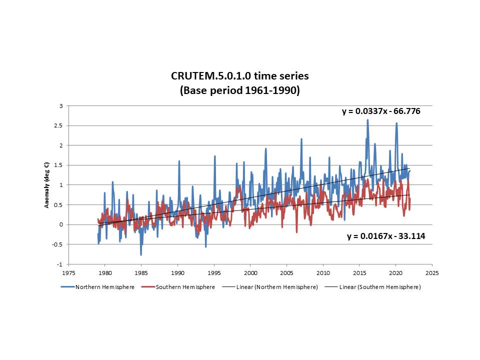
I took a quick look at CRUTEM-5 (air temperature anomalies over land only, as you know) and plotted northern and southern hemispheres separately (since 1979). This shows the northern hemisphere (NH) anomalies increasing at twice the rate of the southern hemisphere (SH): 0.34 C/decade vs 0.17 C/decade. It would be interesting to see UAH (and the models’ forecasts) subdivided by hemisphere. The other issue that shows up is the presence of essentially random spikes in the NH data alone; for the most part these do not correspond to major El Niño events, but they do occur in Jan/Feb/Mar in all cases.
Interestingly, the HadSST3 data also show a divergence of trends between NH and SH but, in that case, it does not show up until 2003, after which the NH anomaly data reflect the seasonal cycle with annual high anomalies in late summer (September, mostly) and low values in winter.
Interesting. The UAH lower troposphere SH and NH overall + their land and ocean averages can be found here:
https://www.nsstc.uah.edu/data/msu/v6.0/tlt/uahncdc_lt_6.0.txt
Caveat! I did this quickly, so would be happy for others to check for errors. Also, note the difference in base period between UAH and CRUTEM-5.
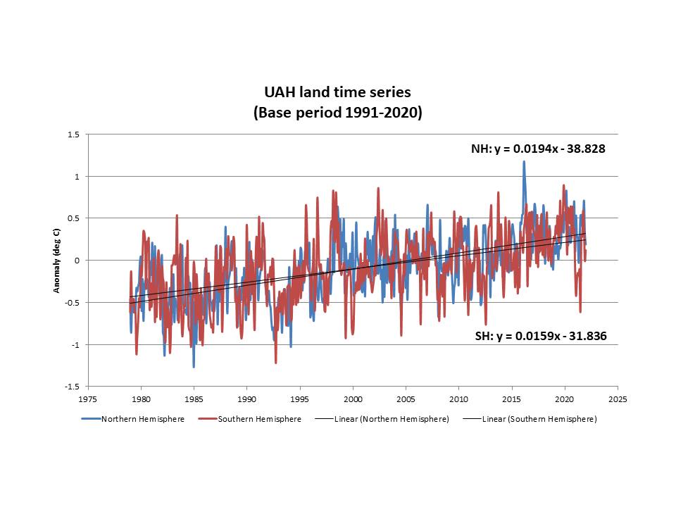
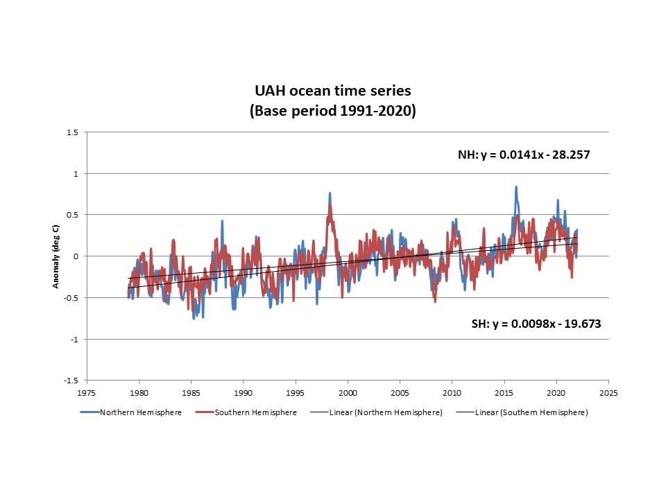
Interesting, thanks for the plots. So, over the ocean, the difference in UAH is 0.0043, or 44%. Over land the difference is 0.0035, or 22%. Smaller difference over land, less heat capacity and thermal inertia, I guess.
I think this needs more analysis. Just visually based on the apparent noise levels, I am not convinced that the UAH trend differences between hemispheres, especially for the land data, are actually significant. On the other hand, the CRUTEM-5 trend data do look significantly different between hemispheres (as do the HadSST3 hemisphere data – not shown here). Proper statistical analysis should help, but it does suggest that there are key differences between the surface and satellite data which need to be better understood – which is pretty much where your post started.
When I looked at the HadSST3 data a few years back, I found a lot of ‘interesting features’; for example, there were temperature values in the base period data for which there were no actual temperature measurements for that cell/month in any of the 30 years of the period. Also, and not too surprising, at higher latitudes in particular (above 60N) there were very large differences in the number of cells with anomaly values between summer and winter, potentially leading to a warm bias in the computed anomalies.
There are some unusual aspects to the UAH global lower tropopause data that don’t show up in the monthly trend graphs. In particular, the baseline averages (in K) that are subtracted from the monthly averages at each grid point (which are then averaged over the entire grid set to get the global average). Thus the output curves are the result of multiple averaging steps. For the baseline averages, there is one set of grid point values for each month of the year. The histograms of these monthly baseline values is quite surprising, this is the February data. The data are barely above 0°C with a large spike of values very close to 0°C. Also shown is the correspond map of the grid point temperatures—the spike values are always in the 30°S–30°N tropics.
Here is the same graph for August:
Your graph is interesting. It suggests that the UAH LT is actually receiving emissions from higher in the troposphere where water vapor is condensing to liquid or ice particles. One might think this level would be close to the top of the troposphere, i.e., the tropopause. Since the LT is a combination of the MT, the TP and the LS products which was originally intended to remove the contamination of the MT due to stratospheric cooling, what does this say about that correction?
Also, the much colder temperatures over the East Antarctic Ice Sheet are a well known result of the high elevations of that region (~4000m), which is reason to reject data from these areas. RSS excludes data poleward of 70S for this reason and their TLT exhibits greater warming as a result.
These are all good questions; you might be correct about water vapor. The LT satellite temperature is a convolution of the sensor responsivity and the 0-10km region where air temperature is rapidly changing. This affects mountainous regions (Asia, SA, Antarctica) where the high elevations come out colder because of lack of signal from the 0-4km altitudes, and these show up in the maps.
I forgot to mention that RSS also excludes other regions with high elevations, including Greenland and scans including the the mountains of the Himalayas and Andes. AIUI, RSS also excluded scans which are anomalously cold due the effects of precipitable ice occurring in strong storm systems, processing which UAH stopped doing with Version 6. One may see these storms in the daily AMSU plots as cold spots.
Why then don’t they exclude hot spots like DIIth Valley or the Sahara? They also exhibit anomalously hot temps compared to other areas around them!
TG, Those areas exhibit few areas with high elevation, thus not any unusual impact on the LT product. Death Valley in particular is below sea-level.
If they eliminate high elevation areas because the cold temps there would bias the global average then why not eliminate hotspots that bias the global average? Remember, they eliminate the high elevation areas not because they are high elevation but because they are cold spots.
No, I think they remove those areas because they radiate at a higher effective pressure level, given the effect of the down welling IR on the surface emissions.
I agree that the spike at 0 C is strongly suggestive of an enthalpy of fusion artifact so your hypothesis makes sense. I’ll have to think about it more deeply though. It might be interesting to see this same graph for the MT, TP, and LS products as well to see if any more useful information regarding the artifact can be obtained.
Values of milli-Kelvin total uncertainty for temperature measurements like these are quite optimistic outside of a calibration lab, count me skeptical.
Of course, both are estimates with the data available at the time. The true uncertainty may never be known. I agree, both estimates are probably low to reality, but we don’t know the reality, do we?
They seem to be measuring precision of the measuring device and not the uncertainty. Kind of like Berkeley Earth does.
Andy,
In order to get uncertainties this low, the various data providers are probably using the Standard Error of the sample Mean calculation. In other words, how close their estimated mean is to the true population means. There is no way these estimates can include MEASUREMENT uncertainty. Measurement uncertainty from multiple measurements always grows, always. If someone says they can “average” away uncertainty, they obviously don’t understand the concept.
“Measurement uncertainty from multiple measurements always grows, always.”
As always it would be helpful if you could provide some evidence to support that assertion.
No, you show that it is wrong.
I tire of giving you references that you ignore. If you have a problem with this you show a reference contradicting it.
You’ve never given me a reference to even suggest that the measurement uncertainty in an average increases as sample size increases.
Do you really want me to show yet again why this is wrong? It is contradicted by the rules of propagation of errors or uncertainties. e.g.
https://www.cpp.edu/~jjnazareth/PhysLabDocs/PropagateUncertainty.pdf
Add the measurements, use Rule 1: Add the uncertainties.
Divide by number of samples, N, to get mean, use Rule 4: Multiply uncertainty by 1/N. (This can be derived from rule 2).
This is the worst case scenario, with no cancelling of errors, and the result is the the measurement uncertainty of the mean is equal to the mean uncertainty of the measurements.
If uncertainties are assumed to be random and independent, you can add the uncertainties using root sum of squares, which will make the measurement uncertainty of the mean decrease with sample size.
Reference: J.R. Taylor Introduction to Error Analysis
Or you could work it out, as I did last year, from the equations given in the Guide to the expression
of uncertainty in measurement
https://www.bipm.org/documents/20126/2071204/JCGM_100_2008_E.pdf
In no case can I see any suggestion that the measurement uncertainty of the mean will increase with sample size.
I’ve shown you multiple times that you do not divide the uncertainty of the sum by n. To find the average you divide the sum by n. Therefore to find the total uncertainty of the average you add the uncertainties of all the elements of the average together, including that of n. Since the uncertainty of a constant such as n equals 0, it does not contribute to the uncertainty. The uncertainty becomes the uncertainty of the sum. There is no rule where you divide the uncertainty by n!
Look at Taylor’s Rule 3.18. There is no division by n. There is an addition of delta-n/n (relative uncertainty) to the total uncertainty. Since delta-n = 0 it neither increases or decreases the total uncertainty.
How much longer are you going to stick with your delusion?
TG said: “Look at Taylor’s Rule 3.18″
Ok, sure.
Let
x = x_1 + x_2 + … + x_N = Σ[x_i, 1, N]
q = x / N
Per Taylor 3.18
(1) δq/q = sqrt[(δx/x)^2 + (δN/N)^2]
(2) δq/q = sqrt[(δx/x)^2 + (0/N)^2]
(3) δq/q = sqrt[(δx/x)^2]
(4) δq/q = δx/x
(5) δq = δx/x * q
(7) δq = δx/x * (x/N)
(8) δq = δx / N
(9) δq = δ(Σ[x_i, 1, N]) / N
Applying Taylor 3.16
(9) δq = δ(Σ[x_i, 1, N]) / N
(10) δq = sqrt[δx_i^2 * N] / N
Applying the radical rule
(10) δq = sqrt[δx_i^2 * N] / N
(11) δq = δx_i / sqrt[N]
TG said: “There is no division by n.”
But there is a division by root-n. Don’t take my word for it. Use Taylor 3.18 and prove this out for yourself.
“Applying Taylor 3.16
(9) δq = δ(Σ[x_i, 1, N]) / N
(10) δq = sqrt[δx_i^2 * N] / N”
Where in Taylor 3.16 is there a division by N?
You already found δq in (8)! δq = δx/N. Then for some reason you want to divide by N AGAIN!
3.16: δq = sqrt[ δx^2 + … + δz^2 + δu^2 + … + δw^2 ]
There is no division by N in this equation!
TG said: “Where in Taylor 3.16 is there a division by N?”
There isn’t. But there is a multiplication by root-N when the uncertainty of all summed elements is the same and there N elements.
TG said: “You already found δq in (8)! δq = δx/N.”
That’s right! δq = δx/N! And δx = δ(Σ[x_i, 1, N]) = sqrt[δx_i^2 * N] = δx_i * sqrt[N]. So δq = δx/N = δx_i / sqrt[N]!
Remember x = x_1 + x_2 + … + x_N = Σ[x_i, 1, N] and q = x / N.
This is nothing more than high school algebra. You can do it. I’ll work through it with you step by step if you want.
TG said: “Where in Taylor 3.16 is there a division by N?”
If there is no division by N then
You are still struggling under the delusion that the standard deviation of the sample means is the uncertainty of the mean calculated from the sample means. Therefore you keep wanting to divide using N.
If all the elements of x have different uncertainties then the sum of their uncertainties divided by N does nothing but equally spread all the uncertainty evenly across all elements of x. You are really finding the mean of the uncertainties. If you have multiple elements in x and they have different uncertainties then the relative uncertainties become δx_1/x1 + δx_2/x2 + … + δx_n/x_n.
If all the elements of x have the same uncertainty then δx = (N * ^x_i). This leads to δq = (N * δx_i) / N so δq = δx_i.
where δq is the uncertainty of the average and δx_i = the uncertainty of each element.
The problems is that you have calculated a uncertainty of a single average value, not the total uncertainty of the elements propagated into that average and you have lost the varied uncertainties of individual elements.
2 rules to remember:
TG said: “1. Why did you quote it as saying that it has division by N?
I didn’t. Regarding Taylor 3.16 and when propagating the uncertainty of a sum what I said is there is a multiplication by root-N when the uncertainty of all summed elements is the same and there are N elements. Don’t conflate multiplication by root-N with division by root-N. Just like sums and averages aren’t the same thing neither is multiplying by root-N and dividing by root-N the same.
TG said: “2. Why are you dividing by N again?”
A division by N shows in steps (1), (2), (7), (8), (9), and (10). Which one are you asking about?
TG said: “You are still struggling under the delusion that the standard deviation of the sample means is the uncertainty of the mean calculated from the sample means.”
This has nothing to do with standard deviation or sample means. I’m using the method YOU prefer (Taylor 3.18). The difference is that I’m doing the algebra correctly while you continue to make trivia mistakes.
TG said: “If all the elements of x have the same uncertainty then δx = (N * ^x_i)”
WRONG. Follow Taylor 3.16 (the rule for sums) step by step. Don’t make stupid high school algebra mistakes. Go slow. Use symbolab.com if you need to avoid making mistakes.
You have defined the following which is not appropriate for what Taylor is trying to teach you.
The equation q = x/N is not a functional relationship. N is a finite number count. It is not a measurement. Therefore your definition doesn’t fit the necessary requirements for this chapter in Dr. Taylor’s book.
Look at the pages I have copied from Taylors book so there is no misunderstanding what he trying to teach you in these examples.
=========================================
First, note the instructions for the example on Page 53 (Eq. 3.8). It says:
This is a functional relationship between measurements. It is not proper to divide by N or the √N, with N being a count of the number of items. N is simply not a measurement used in a functional relationship.
=========================================
Second, let’s address the example on Page 61 (Eq. 3.18 & 3.19. It says:
It goes on to say:
==========================================
Cite: AN INTRODUCTION TO Error Analysis’ THE STUDY OF UNCERTAINTY IN PHYSICAL MEASUREMENTS; 2nd Edition; by De. John R. Taylor; Professor of Physics; University of Colorado
=========================================
I reiterate, this requires a functional relationship between measurements. It is not proper to divide by N or the √N, with N being a count of the number of items. N is simply not an independent measurement with an uncertainty that is used in a functional relationship.
You try to define q(x) as a function but it is not a functional relationship between measurements. It is a simple average, not a relationship that can be used to determine a value. I have tried to point this out before and gave several example of documents that discussed using measurements to determine other intrinsic values.
I urge you to read Chapter 4 in Dr. Taylor’s book more carefully than you obviously have. Chapter 4 more specifically defines using statistical analysis and I urge to stop trying to use equations from Chapter 3 that is based on measurements with uncertainty and the propagation of that uncertainty when multiple measurements are used to define physical quantities. Equations like the Ideal Gas Law or Ohm’s Law are the functional relationships needing Chapter 3 equations.
Please read Page 103 carefully. Two questions to ask yourself are:
1) Does the statistical tools Dr. Taylor uses applicable to multiple measurements of the same thing, i.e. random error?
2) Do these tools apply to measurements of different things like temperatures?
Page 105 addresses this more fully. Such as:
You wonder why you make no headway with folks about uncertainty. You obviously have some math skills but you just as obviously don’t have the physical experience in the world of measurements and making things fit and work properly. Many of us are engineers and are both trained and have experience working with our hands. It is frustrating when folks just don’t get the physical world and how measurements actually work. I would advise you to go talk to a Master Machinist that really makes physical things that must have small tolerances. Have him explain the uncertainties in making measurements and how many times he must throw something away because the uncertainties added up. Using a CAD program to design something isn’t enough. Making it is what counts.
“The equation q = x/N is not a functional relationship.”
Do you understand what a functional relationship is, and if you do could you explain why q = x/N is not one?
“This is a functional relationship between measurements. It is not proper to divide by N…”
Read section 3.4. It specifically explains what happens when you use equation 3.8 with a number that has no uncertainty.
The equation “q = x/N” IS a function. You will get one value out for each independent value put in. However, it IS NOT a functional relationship describing how multiple measurements are used to derive other measurements.
The equation you are using (Eq. 3.18), and Chapter 3 in its entirety, is designed for functional relationships using MEASUREMENTS. The CONSTANTS Dr. Taylor refers to are constants contained in those functional relationships, NOT counts of the numbers of measurements.
You have made an assumption that the equations in question can be generalized into other uses. You need to provide the mathematical proof that shows you can do that. Dr. Taylor does not give you that proof for a reason.
Those constants he discusses are things like C = πd for circumference, A = πr^2, “R” in PV = nRT, u/A = σT^4, or e = mc^2.
If you carefully examine the example Dr. Taylor uses to illustrate the multiply/divide rule for uncertainty you will see the following.
q = (x · … · z) / (u · … · w)
Please, please note, the functional relationship is shown as a [measurement / measurement] and not a division by the count of items measured. Reading and understanding that Dr. Taylor makes a point to not generalize this into finding an average is part of learning. He goes out of his way to tell you that (x thru w) are measurements and not counts.
Dr. Taylor doesn’t even mention the words “means/average” until Chapter 4. Chapter 5 gets even deeper into what the propagation of uncertainty entails and how it works using probabilities.
You are going through a book without an instructor to show you the necessary assumptions and requirements to use different tools. That means you must read EVERYTHING carefully and with UNDERSTANDING. Dr. Taylor consistently tells you the requirements and applies them in the problems at the end of each chapter. I urge you to solve each and every problem to further your understanding.
JG said: “The CONSTANTS Dr. Taylor refers to are constants contained in those functional relationships, NOT counts of the numbers of measurements.”
Just so there is no confusion here I’ve said repeatedly that the most applicable equation to use is Taylor 3.47. The desire to use Taylor 3.18 and treating N (the number of measurements) itself as a measurement with zero uncertainty came from Tim Gorman here. It is important to point out that TG would seen the division by root-N in the final answer had he done the algebra correctly. Anyway, don’t you find it interesting that all of the Taylor equations are consistent with each other though?
Anyone can be led astray and enticed by the mathematics. You are an obvious mathematician with obvious skill to lead someone down the primrose path.
I don’t find it interesting that Dr. Taylor’s equations are consistent. I find that he has presented things in a logical and consistent manner. But as a textbook, I’m sure he expected a teacher would prompt the proper use of the tools he presents.
Your fault is that you deal with the math as a math problem and not a measurement problem. You approach the entire subject from the wrong perspective. It is not about manipulating the math to get the answer you want, it is using the tool to calculate the correct result.
“Taylor 3.47″
Taylor 3.47 *is* 3.18 with the addition of of the partial derivatives of the variables included.
x, … , w are variables, not constants!
Let’s play like N is a valid entry to use in 3.47 so you get:
q = x/N
∂q/∂x = N^-1
Thus there is no ∂q/∂N, the partial of a constant is 0.
So
∂q = sqrt{ [ (N^-1)ẟx]^2 ] }
(N^-1)^2 = N^-2
∂q = sqrt{ (N^-2)( ẟx)^2 ]
(N^-2)^1/2 = N^-1
∂q = (N^-1) ẟx = ẟx/N
This is the exact same equation you already derived from 3.18
You talk about me not being able to do algebra. Tell me where you went wrong here! (hint: what does δq actually equal?)
TG said: “∂q = (N^-1) ẟx = ẟx/N”
YES! You did it correctly! Just being pedantic though…∂q should be ẟq, but I think that was just a typo.
TG said: “Tell me where you went wrong here!”
I see nothing wrong. Remember x = Σ[x_i, 1, N] so ẟx = ẟ(Σ[x_i, 1, N]). That is the correct step.
TG said: “what does δq actually equal?”
Continuing from where you left off:
(1) ẟq = ẟx/N
And because x = Σ[x_i, 1, N] then:
(2) ẟq = ẟx/N = ẟ(Σ[x_i, 1, N])/N
We then apply Taylor 3.16 to solve for ẟ(Σ[x_i, 1, N]) to get:
(3) ẟ(Σ[x_i, 1, N]) = sqrt[ẟx_i^2 * N] = ẟx_i * sqrt[N]
We then plug that back into (2) to get:
(2) ẟq = ẟx/N = ẟ(Σ[x_i, 1, N])/N
(4) ẟq = (ẟx_i * sqrt[N]) / N
We then apply the radical rule to get:
(5) ẟq = ẟx_i / sqrt[N]
“ẟ(Σ[x_i, 1, N]) = sqrt[ẟx_i^2 * N] “
really?
ẟ(Σ[x_i, 1, N]) = ẟx, this does not require all the x_i values to be the same.
And it really should be (Σ(ẟx_i), 1, N) which is ẟx
sqrt[ẟx_i^2 * N] , why did you square ẟx_i but not N? And this also requires all ẟx_i values to be the same where the generalized form does not.
perhaps this should be sqrt{ (ẟx_i * N)^2 } which again equals ẟx
In any case it all winds up with ẟq = ẟx/N. the same thing we started with plus a whole bunch of unnecessary manipulations.
We still wind up with ẟq_avg = ẟx_total / N
Tell me again about my algebra errors?
in general, ẟq_avg is meaningless for measurements of different things using different measurement devices, x_avg is meaningless and so is ẟx_i = ẟx_total / N. When you have different things being measured by different things you will probably not wind up with a Gaussian distribution of x_i or ẟx_i. You can have skewed values including multi-modal distributions. Multi-modal distributions are not well described using typical statistical parameters and neither are skewed distributions.
You are still stuck with that one, single hammer you have in your tool belt. Throw it away and get a complete tool collection.
bdgwx said: ““ẟ(Σ[x_i, 1, N]) = sqrt[ẟx_i^2 * N]“
TG said: “really?”
Yes. Really. That’s what the RSS (Taylor 3.16) rule says.
TG said: “And it really should be (Σ(ẟx_i), 1, N) which is ẟx”
That’s not what the RSS (Taylor 3.16) rule says.
TG said: “sqrt[ẟx_i^2 * N] , why did you square ẟx_i but not N?”
Because that’s not how the RSS (Taylor 3.16) rule works.
TG said: “We still wind up with ẟq_avg = ẟx_total / N
Tell me again about my algebra errors?”
Show your work…step by step.
“That’s not what the RSS (Taylor 3.16) rule says.”
3.16 is for sums and differences.
3.18 shows sqrt{ (ẟx/x)^2 + (ẟN/N)^2 | = ẟx
3.46 shows the same thing: [ (1/N)(ẟx) ] ^2
Your lost in your own math.
TG said: “3.16 is for sums and differences.”
Yep! And x = Σ[x_i, 1, N] is a sum! So to solve for ẟx you use Taylor 3.16. Optionally you can use the more general partial differential technique via Taylor 3.47.
TG said: “3.18 shows sqrt{ (ẟx/x)^2 + (ẟN/N)^2 | = ẟx”
Wrong. sqrt[(ẟx/x)^2 + (ẟN/N)^2] = ẟx / sqrt(x).
TG said: “3.46 shows the same thing: [ (1/N)(ẟx) ] ^2”
First…[ (1/N)(ẟx) ] ^2 is not the same thing as the wrong answer of ẟx or the right answer ẟx / sqrt(x).
Second…it is hard to tell what you are doing here because you are omitting the = sign so I can’t tell what you think [ (1/N)(ẟx) ] ^2 is even supposed to be.
You need to slow down and take each step carefully. Show all of your work and don’t make simple algebra mistakes like you just did above. Use symbolab.com if you need to. It will do the algebra for you.
Remember x = Σ[x_i, 1, N] and q = x / N and the goal is to solve for ẟq.
“The equation “q = x/N” IS a function. You will get one value out for each independent value put in. However, it IS NOT a functional relationship describing how multiple measurements are used to derive other measurements.“
Then you should be clear that’s what you meant, instead of just throwing words like “functional relationship” around.
So what are you saying here? That a mean is not a derived measurement? You still haven’t explained how any of this is meant to prove that uncertainties always increase with multiple measurements.
Do you regard the sum of multiple temperature measurements to be a “functional relationship describing how multiple measurements are used to derive other measurements.”? Because that seems to Tim’s logic. No problem with using propagation of errors to derive the sum, but for some reason cannot divide the uncertainty of the sum by N to get the uncertainty of the mean.
The sum of multiple temperature measurements is not a functional relationship unless it accomplishes the output of some type a measurand.
The GUM, Section 4.1 starts with this:
The simple sum of multiple temperature measurements does not result in “a measurand Y”. The division of a sum of multiple temperature measurements divided by a count of the number of measurements does not result in a measurand, it only results in a “means” which is a statistical parameter denoting the center of a group of data. It is not a measurand, it is a statistical parameter.
Read the GUM definition carefully and give it some thought. Here are some measurands determined from “N” other quantities denoted X1, X2, … Xn.
V=IR
PV = nRT
E = mc^2
Area = L x W
Circumference = πD
Volume = L x W x H
Perimeter = 2(L + W)
What do you call a sum of multiple temperatures? I guess you could say Total Temperature = T1 + … + Tn, but is that a real physical measurand determined by other measurements? Does the Total Temperature of your group of data provide a “measurand”?
If I tell you that the total height of all the animals in a herd is some number, is that a measurand? I suppose it might be if you were building a fence and needed to know how high it needed to be in case the animals learned to form a stack of one on top of the other.
Give up trying to minimize the total uncertainty of the mean of a group of temperature data. Accept the fact that dividing by “n” is statistical calculation to provide the precision of the mean and not its uncertainty. Dr. Taylor even downgrades this.
Please note, this only covers measurements of the same thing in case you were thinking is could be used to calculate the uncertainty of temperature measurement based upon both time and location.
I get the feeling you are only looking for equations and not really studying Dr. Taylor’s book. Have you worked out the answers to all of the problems at the end of each section? Doing so will provide you some insight about what is going on.
Believe me, you will not find anything in Dr. Taylor’s book nor the GUM that deals with the uncertainty with a group of measurements that are not of the same thing.
The reason I’m asking about the sum of temperatures is because you still haven’t explained why you think that the uncertainty increases with more measurements. The only explanation offered is that uncertainty increases as you add measurements, using the propagation of uncertainty rules, but you cannot divide that uncertainty when you take an average because it’s not a measured value.
Everything else you are saying is a distraction from your failure to offer any reason for why you think “Measurement uncertainty from multiple measurements always grows, always.”.
“The equation you are using (Eq. 3.18), and Chapter 3 in its entirety, is designed for functional relationships using MEASUREMENTS. The CONSTANTS Dr. Taylor refers to are constants contained in those functional relationships, NOT counts of the numbers of measurements.”
And why exactly do you not think the count of measurements is not a constant used in the functional relationship defined by the mean function? Why can you not accept the count as a measurement without uncertainty?
“You have made an assumption that the equations in question can be generalized into other uses. You need to provide the mathematical proof that shows you can do that. Dr. Taylor does not give you that proof for a reason.”
If Taylor thinks there are exceptions to the rules then he should have stated them. Everything follows from the propagation of errors, it makes no difference to the maths of you don’t like the conclusions.
“Those constants he discusses are things like C = πd for circumference, A = πr^2, “R” in PV = nRT, u/A = σT^4, or e = mc^2.”
And also like dividing the measurement of a stack of 200 sheets of paper by 200 to get the width and uncertainty of a single sheet.
“Please, please note, the functional relationship is shown as a [measurement / measurement] and not a division by the count of items measured.”
And again this all hangs on you thinking you can pick and choose what a measurement is. Counting is not apparently a measurement, but pi is.
“Why can you not accept the count as a measurement without uncertainty?”
I have not read the dozens of back and forths for comprehension, but this caught my eye. Look at any of the many primers on basic statistical data processing, and they emphasize that:
If Mr. Gorman is so blocked as to miss this fundamental truth, then, while I admire the patience of you both, I also agree with you that:
“I have no expectations that the following corrections will make any more impact on you than all the many times I’ve explained this to you and Jim before. They are simply here for the benefit of any passing reader.”
“Why can you not accept the count as a measurement without uncertainty?”
If it has no uncertainty then it can’t add to, subtract from, multiply by, or divide into the total uncertainty.
In Taylor’s equations, δq/q = sqrt[ δx^2/x + δN/N ] where δN = 0
δq/q ≠ sqrt[ [(δx)/x]^2 / N ]
δq/q ≠ sqrt[ (δx/x)^2 ] /N
This is true even if you violate Taylor’s restrictions and assume that N is a measurement.
“And also like dividing the measurement of a stack of 200 sheets of paper by 200 to get the width and uncertainty of a single sheet.”
That is a calculation, not a functional relationship. A functional relationship requires a variable of some kind. δq is a measurement, not a variable. δq/B = δx is a calculation using one measurement to get another. That’s not a functional relationship, it is a calculated value.
TG said: “If it has no uncertainty then it can’t add to, subtract from, multiply by, or divide into the total uncertainty.”
The use of Taylor 3.18 and treating N as a measurement was your idea.
Bellman and I have been saying along that the more appropriate application in this case would to use the partial differential method by setting q = Σ[x_i, 1, N] / N and use Taylor 3.47 or set f(x_1, …, x_i) = Σ[x_i, 1, N] / N and use GUM 10.
The partial differentiation formula gives you the same answer.
ẟq/ẟx = 1/N
ẟq = sqrt{ [(ẟq/ẟx) ẟx]^2 } = sqrt{ [ (1/N)ẟx)]^2 } = sqrt{ (ẟx/N)^2 } = ẟx/N
You need to correct your algebra.
TG sadi: “ẟq/ẟx = 1/N
ẟq = sqrt{ [(ẟq/ẟx) ẟx]^2 } = sqrt{ [ (1/N)ẟx)]^2 } = sqrt{ (ẟx/N)^2 } = ẟx/N”
Yes! Now solve for ẟx to find the final answer.
Remember x = Σ[x_i, 1, N]. You can use the same partial differential procedure (3.47) or the familiar root sum square rule (3.16) to find ẟx.
“If it has no uncertainty then it can’t add to, subtract from, multiply by, or divide into the total uncertainty.”
How many more times do we have to go around this with you still missing the point?
When you add the uncertainty of N you are adding zero, so it has no effect on the result, but it’s what you are adding to that makes the difference. You are adding zero to he FRACTIONAL uncertainty, so the FRACTIONAL uncertainty remains unchanged. This mean that because q does not equal x, that means that δq does not δx, and in fact means that δq = (q δx) / x = δ / N.
As you insist you don;t understand mathematics, let’s look at a hypothetical example. Say you find 100 planks of wood in a ditch and want to know what their average length is. You measure each plank and add them together, and also work out the uncertainty. Say the total length is 152 ± 1m.
So you divide this sum by 100 to get the average length, 1.52m. What’s the uncertainty of that average. Using the rules for propagation we get
δq / q = δx / x + 0
here q is the average length and is the sum.
so,
δq / 1.52 = 1 / 152
which means
δq = 1.52 / 152 = 1 / 100
So the mean is 1.52 ± 0.01m.
The example of the sheets starts with the basic assumption that “ALL SHEETS ARE EQUAL”. There is no “average”.
Does your example start with the same assumption?
What is the distribution when all the data points are the same? What is the distribution for your example of temp anomalies?
Once again, as you are obsessed with this and and failing to understand my point. You claimed it was impossible to divide an uncertainty by a count as it wasn’t a measurement. When I point out that Taylor gives examples where he does just that, you change the argument to “but that’s not an average” as all the sheets are the same. All the time shifting the argument to distract from the fact that you have done nothing to prove your claim that ““Measurement uncertainty from multiple measurements always grows, always.”
Measurement uncertainty from multiple measurement does always grow.
You are trying to show that uncertainty can be reduced by dividing by a count. All that does is assign the same reduced uncertainty value to each and every member. Consequently, the necessary requirement that all members have the same value and uncertainty.
Does each of your data points have the same value and uncertainty? If they don’t, then this example doesn’t apply.
Here is how a person like you approaches it using your example of boards. Say you collect 2×4’s and you have 1000 of them. A contractor wants to buy them. You have measured them and gotten an average length of 8 ft. But you know that you can also average the +/- 2 inch variation by dividing by 1000. So you tell the contractor my assortment of 2×4’s average 8 ft +/- 0. 002 inches.
Is the contractor going to be happy?
Is he going to understand that you just assigned the same uncertainty to each board in the bundle?
“Measurement uncertainty from multiple measurement does always grow.”
Yet after dozens of posts, you’ve still yet to provide any evidence for this. The best you can do is insist the rules for propagation of uncertainties don;t apply to taking an average. But even if that is the case you need to explain what rules should be used and how they result in an increase in uncertainty.
(Of course, if you mean the uncertainty of the sum increases, then I’m not disagreeing. It’s just not a useful argument.)
“Here is how a person like you approaches it using your example of boards. Say you collect 2×4’s and you have 1000 of them. A contractor wants to buy them. You have measured them and gotten an average length of 8 ft. But you know that you can also average the +/- 2 inch variation by dividing by 1000. So you tell the contractor my assortment of 2×4’s average 8 ft +/- 0. 002 inches.”
Once again, I don’t. I’ve explained before how the best use of the ± value depends on what you are describing, and how it can be misleading if you are reporting the standard error of the mean, but the user expects it to be the standard distribution of the population.
(Besides, a person like me would not be using an antiquated measuring system.)
To see if I’ve got this correct though, I’ve measured 1000 boards with an average length of 8′, and the sum and uncertainty in the sum of those boards is 8000′ ± 0.167′.
What I don’t know from you example is what the standard deviation of the boards was, I just know with a surprising high degree of precision that the sum came to 8000′ give or take a couple of inches. I can’t tell you how how likely it is that any random board will be within a few inches of 8′.
“Is the contractor going to be happy?”
Depends on what the contract required. If it required all boards to be close to the 8′ figure than probably not, but we don;t know because you didn’t state what the deviation of the boards was. It may be they are all the same length, and given the total came to exactly 8000′ that may be likely, but we can’t know for certain without you giving more details.
If the requirement was that they get 1000 boards with a total length of 8000′, then that might be acceptable. Again you’d have to show me the contract to know for sure.
“Is he going to understand that you just assigned the same uncertainty to each board in the bundle?”
That is not what I’ve done. I’ve stated a value for the average with a small measurement uncertainty. That is a statement about the average length of the board, not a statement about the uncertainty of each board.
That is correct. what is the standard deviation of the temperatures you are finding the average of. Not anomalies, but the actual temperatures. The anomalies should carry the same variance as the original temps to be able to accurately assess what the variation is.
Why? Because of the following.
Have you propagated the sigma(ran)+sigma(sys) through from the absolute temps into the anomalies and then into the average of anomalies?
“That is correct. what is the standard deviation of the temperatures you are finding the average of.”
I don’t know, it’;s a hypothetical example. But it’s irrelevant for what keeps being discussed, which is measurement uncertainty. I’ve tried to explain numerous times that the real uncertainty in a sample mean is that which is caused by the random sampling and not to any extent the measurements.
But everything keeps being explained to me in terms of propagating the measurement uncertainties, how they increase the uncertainty of the sum, but don’t decrease when you take the average. Hence why I keep adding the word measurement to any description of these uncertainties.
The rules from propagating uncertainties are about measurement uncertainties and show that the measurement uncertainty of a mean will be equal to the individual uncertainty of a measurement divided by the square root of N. (assuming all uncertainties are random and independent and are the same size for each element). It’s this you Tim and Carlo keep disputing.
The real uncertainty I maintain is the SEM, which is determined by dividing the sample standard deviation by the square root of N. (Again this assumes that all samples are random and independent).
It’s no coincidence that these equations are the same, and you can look at the SEM as doing the same thing as propagating random errors. Each sample can be seen as a random measurement of an average size. But as the deviation of individual elements is usually much bigger than the deviation caused by the error in a measurement it gives a bigger uncertainty of the mean.
“what is the standard deviation of the temperatures you are finding the average of. Not anomalies, but the actual temperatures. The anomalies should carry the same variance as the original temps to be able to accurately assess what the variation is.”
More nonsense. Of course the standard deviation of anomalies will be smaller than of absolute temperature. Anomalies reduce variations in temperature by comparing them to a local base. Local both geographically and seasonally. You’ve only got to look at a map of monthly global anomalies to see how much less variation there is than you’d get with absolute temperatures.
“Why? Because of the following.”
The following being a brief mention of systematic errors.
How does that suggest that anomalies should have the same standard deviation as absolute temperatures? If anything anomalies help to reduce systematic error. If a thermometer is always too hot, both it’s current temperature and the base temperature will be too hot, and so the systematic error cancels. (I’m not suggesting that will always happen. Systematic errors that change over time are the real problem.)
“Have you propagated the sigma(ran)+sigma(sys) through from the absolute temps into the anomalies and then into the average of anomalies?”
I’m not doing anything. I’m just trying to get you to give some evidence that “Measurement uncertainty from multiple measurements always grows, always.”
I intended that the uncertainty of each board be +/- 2 inches. I screwed up the example.
BTW. You say I’ve measured each board and the uncertainty of the sum was ± 2″, correct? So what was the uncertainty of each measurement? Depending on how this was added you have to assume the precision of these individual measurements was high, uncertainty of ± 0.002″ if we are just adding the uncertainties, or if we assume random errors then ± 0.063″.
Do you think it’s appropriate to claim the measurement uncertainty of the average board length is actually ± 2″? How does increasing the number of boards increase the uncertainty? Say I have 1000000 boards with a total length of 8000000 ± 2000″. Does that make the uncertainty of the average 8′ ± 170′?
“Reading and understanding that Dr. Taylor makes a point to not generalize this into finding an average is part of learning.”
Which brings us back to square one. Either an average is a derived measurement and the rules for propagating uncertainties hold, or it isn’t in which case we can ignore all those rules, and you need to explain what rules you want to use to prove “Measurement uncertainty from multiple measurements always grows, always.”
“He goes out of his way to tell you that (x thru w) are measurements and not counts.”
Here’s what Taylor says about equation 3.9: (My emphasis)
How do you use this if counting is not allowed?
He also says:
Why is this statement made? Maybe the individual sheets also have equal uncertainties? Do temperatures you are dividing all have an equal value? What does the distribution of all equal thickness sheets look like? What is the standard deviation? Are all the temperatures in your sum equal? Are the uncertainties of each member of the sum equal?
Lastly, look at the process in this example. The total height of the group is measured and the total uncertainty is determined. This is then translated into equal measurements of each sheet. And, the uncertainty of the actual total measurement is then equally apportioned to each element. Here is the process.
1) Assume all sheets are equal.
2) Measure total height
3) Calculate total uncertainty
4) Allocate the total height and uncertainty to each member.
You are trying to make a different process equivalent to this. Do you consider the sum of a group of temperatures to be a MEASUREMENT of the TOTAL TEMPERATURE? Are the uncertainties of each temp measurement the same? Here is your process.
1) Measure each member.
2) Determine the uncertainty of each member.
3) Sum all member’s temperature and uncertainty.
4) Reallocate temperature and uncertainty to each member equally by using averaging.
Here are two very pertinent questions.
1) What is the standard deviation of the sheet distribution? (Each sheet equal)
2) What is the standard deviation of the sum of temperatures? (Each temp not equal)
Do you see the difference in each procedure?
Chapter 4 addresses the difference between error analysis and statistical analysis. You need to read it.
“Why is this statement made?”
Because he’s not talking about finding the average width of different sheets of paper.
Stop evading the issue and explain why you think N being a count invalidates the equation, and then show your evidence that ““Measurement uncertainty from multiple measurements always grows, always.”.
Did you not read the assumption in the example that all sheets are equal thickness?
Are you assuming all the temp anomalies are the same?
Did you miss the issue that Dr. Taylor’s example starts with a measure of the whole stack and the total is distributed in equal measure to each part.
Is your method starting with a MEASUREMENT of the entire temperature that has an uncertainty.
Does the example find an “average”? How is that possible? Maybe because all the sheets are equal; huh?
“Did you not read the assumption in the example that all sheets are equal thickness?”
I just told you why he wants to make that assumption. I’ve also told you why these distractions won’t work.
You make a claim about how the uncertainty of an average increases with the number of measurements – you are failing to provide any evidence to back it up. We show you how the the rules of propagating uncertainty imply that sample size will either leave the uncertainty unchanged or for random errors decrease it. You object on the ground that those rules don’t apply to the case of dividing by a count. I show you where Taylor does just that, and you try to shift the goal posts again.
If you don’t think these rules can be applied to an average, or to an average of different sized things or whatever, then you have to a) give a reason for those exceptions, and b) show what the correct rules are and how they can be used to show uncertainties increasing with sample size.
“Did you miss the issue that Dr. Taylor’s example starts with a measure of the whole stack and the total is distributed in equal measure to each part.”
More distracting. You said that that you couldn’t use the rule for q = x / N, on the grounds that N wasn’t a measure. Now you seem to agree you can use the rules, but only if you measure the total in a single go, not if you get the total by adding the individual elements. Is this really what you think?
“Does the example find an “average”? How is that possible? Maybe because all the sheets are equal; huh?”
Yes it does find the average thickness of a sheet of paper in the stack – that’s the definition of the mean average. Of course, if all sheets have exactly the same thickness then that will be the same as the average, and you can say you’ve found the thickness of an individual sheet.
As an aside, I don’t know how exactly equal you want all sheets. I doubt if there are two sheets in the world with exactly the same thickness, let alone 200, and unless you measure every sheet you will never know. I suspect a reasonable person would assume that the point of that remark is that all the sheets are of similar thickness, say because they’ve all come from the same pack, rather than mixing different types of paper.
You are trying to apply tools that don’t apply. BTW, when you sum for an average, the uncertainty grows.
Chapter 3 covers uncertainty in measurements used to calculate a final value. The generalized versions used in this chapter do not require equal measurements or uncertainties. The one example in which a “count” is used also has a very explicit assumption, all members have equal measurements and uncertainties. Chapters 8 and 9 will provide the mathematical basis for the requirement.
Chapter 4 introduces “means” and associated errors/uncertainties but guess what, it has a very explicit assumption also. Repeated measurements of the same thing.
Chapter 5 introduces statistical analysis of repeated measurements of the same thing along with a normal distribution.
You might read chapter 7 to get an idea of consistency. You’ll notice that technically this chapter also requires a single physical quantity.
You are trying to justify your use of statistical analysis of different things from chapters in a book that don’t apply.
As I have said before, sampling and/or time series analysis are a more appropriate venue than pure simple statistical analysis.
JG said: “You are trying to apply tools that don’t apply.”
That’s what we keep hearing.
Carlo, Monte tells me I have to use the GUM to propagate uncertainty. I use the GUM 10 and get u(Tavg) = u(T) / sqrt(N). He disagrees and uses GUM 10 only to make an algebra mistake which, if corrected, also yields u(Tavg) = u(T) / sqrt(N).
Tim Gorman tells me I have to use Taylor. I use Taylor 3.47 and get δTavg = δT / sqrt(N). He say you have to use Taylor 3.18 and treat N as if it were a measurement with no uncertainty only to make an algebra mistake which, if corrected, also yields δTavg = δT / sqrt(N).
Pat Frank tells me I have to use Bevington. I use Bevington 3.14 and get σTavg = σT / sqrt(N). He says nope and points me to Bevington 1.9 which is nothing more than the well known variance formula which not only does not propagate uncertainty, but does not agree with the formula he used in his paper.
At this point I have no choice but to believe that each of you was okay with the GUM, Taylor, and Bevington until you saw that they didn’t give you the result you wanted.
“BTW, when you sum for an average, the uncertainty grows.”
Yes, as we’ve been saying all along. For some reason you think the uncertainty of the mean is the same as the uncertainty of the sum. That’s one of your problems.
“You are trying to justify your use of statistical analysis of different things from chapters in a book that don’t apply.”
And here we go again.
When this began I’d never heard of the Taylor book. I just explained it was self evident that you had to divide the uncertainty of the sum by N to get the uncertainty of the mean.
Then when that fails and it’s obvious that Taylor, along with every other source on metrology, agree with me. Surprise, it turns out Taylor can’t be applied to the uncertainty of a mean after all.
So, we go back to the question – if we cannot use Taylor to tell us what the uncertainty of the mean is, what do you use? How do you establish that the uncertainty should increase with sample size?
Check your books. You are trying to average things that are single measurements of different things. Most books on error and uncertainty don’t deal with this. If you can find a book that deals with averaging different measurements of different things, at different times, with different devices please let me know. I think the closest thing you will find is sampling theory or time series analysis. And, the vast majority of that kind of information doesn’t deal with how to assess uncertainties of measurement. They simply assume all the data is 100% accurate.
Dr. Taylor says that you must break down the uncertainties into random and systematic. I know most climate scientists and apparently other fields also want to ignore the systematic uncertainties that statistics won’t resolve. In measurements you need to deal with the resolution of the instruments and the uncertainties from that. Random uncertainties (and random errors) can be dealt with through statistics but even those have certain restrictions.
Read the following and pay attention to #4, #5, #8, and #10.
https://citeseerx.ist.psu.edu/viewdoc/download?doi=10.1.1.496.3403&rep=rep1&type=pdf
Another document that talks about the SEM.
https://watermark.silverchair.com/aeg087.pdf?token=AQECAHi208BE49Ooan9kkhW_Ercy7Dm3ZL_9Cf3qfKAc485ysgAAArswggK3BgkqhkiG9w0BBwagggKoMIICpAIBADCCAp0GCSqGSIb3DQEHATAeBglghkgBZQMEAS4wEQQM3WgDo3YOkP6vFY2hAgEQgIICbkKbBlqrm7SRhmGbOwzWPFFB1qC-ZmYUYxhtVx8Xx8TUaVUZwXbLJvOTXNYzSzNB8atpd9xJft6giDM2JKNSthw2MHOUczUjcOztrIQHS2NLf_L1AZmQEB1UCm1JXv_8URESJ9EtyqzGXWnMxmkFsCmmQ6LL2-rEUDUwhqSz-B1qXz5F36i4uY08T8vAIylph2WBmwsMnbXQqCO6uvLbcgO_4J4vjkzEwV-SCJhAI1J9mceRK_7ipGCSvl01wwhKNu8wf-L0dW5LGpNbkrc-iAuYbg_TodYBz0WaUEg_x9jPEkmLs3fG2nS2zdArAzw_XDPax6Nn4ryzihuXv7LRB5MowymKNvB3vOuOW5nAkL0b8ZLPnupgfj25N06W5A8GjVFqKLG09STD6HgAR8Zsw4fJlcbpcEw2JCvMqFrageJvr5YeZW7Gco8acDX14VRnXjVZc2jbwxuMREeEp2RCZ2hAhT0Qfybwcsg-R2t0xn4dw3rMQzGYhfCWki9VMByPrA_pXCx7iBmni0Kxqf0qKyKqOevLYQhi_nOrIBJdq8BEmkO5wBd-CV-BOlAYka7YU04cK5YKwf9maxGRZrkoFM9HsUcenfJ8tHfvYWQu19LK9rFuKfcwPcFgglslIpVeuompxI1u-0-rUhkq2ZpIIBqRseyJDbftn0SVy7PYXw4PCCP9eff9e2oQgxdT6Wy_oczBNY7FWndUw18U_ZqfjueobDoF-mMqCo96THARuzpWiiQOywIP-wb1avlpCFyP1eWksAWEq6fE6JDE3YHTznSpv0_UwSFG6aTWwQ6nwqylptQ67Y6WfQ2FZZir71M
“You are trying to average things that are single measurements of different things. Most books on error and uncertainty don’t deal with this.”
Yet you keep trying to use those books to claim that measurement uncertainty increases sample size. It’s your claim, you need to provide the evidence.
“And, the vast majority of that kind of information doesn’t deal with how to assess uncertainties of measurement. They simply assume all the data is 100% accurate.”
Try thinking through the problem rather than expecting books to tell you everything. What is the uncertainty of the mean assuming exact measurements? What is the uncertainty caused by measurements alone? What happens if you combine them? Do you need to combine them, or is the fact the measurement errors are already present in your data mean they were already accounted for in the sample deviation? Maybe run simulations to test these questions.
Your second link is broken. I’m not sure what your point is with regard to the first link. It’s nothing I disagree with. Statistics are complicated and easy to get wrong and misinterpret. None of this supports your claim that measurement uncertainty increases with additional measurements.
“As I have said before, sampling and/or time series analysis are a more appropriate venue than pure simple statistical analysis.”
I’ve been saying this throughout. The uncertainty of the mean is mainly about the uncertainty coming from the random sampling. That is simple statistical analysis. The uncertainty of the mean usually has little to do with the uncertainty of the measurements. When your random samples vary by 10 or 20°C what effect do you think a 0.5°C error in each measurement will have? But whenever I say this someone says I don;t understand metrology and the problem with statisticians is they assume all measurements are exact.
However, and it’s a big however, it makes no difference to your claim that increasing sample size will increase the uncertainty. The uncertainty of the mean, by which I mean the standard error of the mean still decreases as sample size increases.
Nor does it help your argument to switch to saying it’s the standard deviation of the population that is the true uncertainty of the mean, because that doesn’t generally change with sampling size.
See this. https://wattsupwiththat.com/2022/03/15/satellite-and-surface-temperatures/#comment-3482184
My biggest problem has always been seeing temperatures of 0.00# when anomaly temps are quoted. You simply can not have that kind of precision from instruments whose resolution only allows +/- 0.5 systematic uncertainty. 1/100th or even 1/1000th is too far inside the uncertainty interval to mean anything.
Dividing by N is just finding a statistic that is small enough to look good. The papers from the above should tell you that. Dr. Taylor should teach you that the uncertainty from LIG thermometers outght to be considered systematic and carry through any calculations using them.
The implicit assumption in using an average is the same as in Dr. Taylor’s sheet example. EACH MEMBER OF THE GROUP HAS EQUAL MEASUREMENT AND EQUAL UNCERTAINTY.
Let’s examine that. As I tried to point out his example starts out with a total measurement and the assumption that all the sheets are the same.
You on the other hand start out with large number of anomalies that are explicitly different in both value and uncertainty and then add them to a whole measurement by adding them together. Then you calculate an average that implicitly spread the differences among all the members.
That is one reason so many scientists and politicians assume everywhere is warming the same. How many studies have you read that indicate Climate Change is going to affect a local harvest, population count, or rainfall. That is because the average is spread out to everywhere.
An hypothesis only takes one instance to prove it invalid. Are you going to maintain that an average that is spread out over the entire earth is valid? You only need to examine the points that are used in the average to know that isn’t true.
As an engineer should I accept an average measurement and associated average uncertainty (tolerance) in a product that has a safety concern. Or, should I also ask for a standard deviation of the product measurement?
“The implicit assumption in using an average is the same as in Dr. Taylor’s sheet example. EACH MEMBER OF THE GROUP HAS EQUAL MEASUREMENT AND EQUAL UNCERTAINTY.”
Nonsense. There’s no requirement that average can only be taking from things with the same size. It’s generally assumed that they will be different sizes or else there would be little point in taking an average. If you know they are all the same, you could just measure one thing.
I think your problem is trying to reduce everything to engineering terms. If you are only looking at averaging as way of reducing errors in measurement then yes, you want everything to be the same size. But there’s a whole world outside the engineering workshop, where averages have are used for different purposes.
Even in the engineering arguments, it’s never clear exactly what everything has to be the same means. Sometimes I told you can only take an average if you measure exactly the same physical object object with the same instrument, and same observer, under identical conditions.
Other times it can be multiple objects as long as you have a reasonable expectation they are all roughly the same size, as in the stack of paper.
Other times it’s possible to measure different sized things as long as you are using them to derive a constant, as in the spring and weight experiments.
Other times, you can take the mean of random different sized measurements in order to get an average that is assumed to be constant but random, such as radioactive decay.
Do temperatures have a reasonable expectation of being roughly the same?
Of course it is ok when you are trying to determine a constant value within a functional relationship. But did you see the uncertainty be divided by N = the number of samples to determine the total uncertainty. The spring example I looked at in Section 4.5 used the Standard Deviation as the uncertainty, not any specific uncertainty in the measuring devices. He even said that if you could determine the reasonable uncertainties in the individual measurements used in the experiment, mass and time, you should see similar values. Please note that would include both random and systematic uncertainties.
Chapter 11.1 discusses random radioactive decay. Please note this requires probability calculations and Poisson distributions. Not sure this is a good example of finding uncertainties of measurements.
“Let’s examine that. As I tried to point out his example starts out with a total measurement and the assumption that all the sheets are the same.”
You keep misunderstanding the point of the general argument. I’m not saying the stack of paper example is identical in operation to averaging temperature readings. The point was that you insisted the general Taylor rule 3.9 did not apply when the constant was a count. The stack of paper example unambiguously shows it can be a count.
“That is one reason so many scientists and politicians assume everywhere is warming the same.”
How many do that? Anyone who follows and understands the evidence knows that’s not the case. You can easily check the data to see that land is warming faster than ocean, that the northern hemisphere faster than the southern one. You can check out the GISS maps to see how much different parts of the world have warmed or cooled since any date.
The only people I see making that assumption is some here who will argue that 1.5°C warming isn’t bad as it will just mean where they live will be a little warmer, or those who keep searching for any small corner of the globe that hasn’t warmed over a certain period and suggest this means there is no global warming.
Read that rule again, especially, “measuring something”.
Now tell me how an average is “measuring something”.
The rule says nothing about q needing to be “measuring something”. Rule 3.9 says
As I’ve said before, I don;t really care if you classify a mean as a measurement or as a calculated value. But if you insist that it’s not a measurement, then stop claiming you have to follow the rules of metrology to determine its uncertainty, and show me what rules you want to use, that prove “Measurement uncertainty from multiple measurements always grows, always.”.
It’s obvious you don’t care. However Dr. Taylor’s Chanpter 3 starts with the following.
Exactly what “one or more” quantities are you measuring directly?
Does Dr. Taylor’s sheet example have a direct measurement involved?
“Exactly what “one or more” quantities are you measuring directly?”
The individual elements obviously. If we take Tim’s 100 thermometers example, the things would be the 100 temperature readings.
“Does Dr. Taylor’s sheet example have a direct measurement involved?”
Yes, the height of the stack. I’m really not sure where you are going with this.
You are not following the procedure in the example which is measuring the total temperature. By finding the total height and dividing by the number of sheets, Dr. Taylor assigned the same value and uncertainty to each member. That is why the necessary assumption that each member has equal height and uncertainty as the average.
The standard deviation of the example is zero. What is the standard deviation of your data? Do you not see the difference?
You are doing a circular reasoning to rationalize what the average uncertainty is. What do you think the resolution of a device that could measure the temperature of the entire earth would be? What do you think the uncertainty in that measurement would be. That would be equivalent to the example.
There is also an important caveat in Dr. Taylor’s book that you probably haven’t read.
The resolution of an instrument has much to do with the systematic uncertainty. It goes to how data is read from the instrument and the number of Significant Digits recorded.
Since most data from LIG thermometers before, say, 1980 was recorded only with integers, this must be considered as the minimum systematic uncertainty for each measurement, i.e., +/-0.5. Consequently, an average of these temperatures will carry the systematic error since it can not be reduced by statistical analysis, only better equipment or techniques. It also means that this is the minimum uncertainty since other factors can increase it.
Remember, the other point is that all of Dr. Taylor’s book and the GUM deal with multiple measurements of single things, be they an actual single physical object or the same experiment done over and over with the same equipment and techniques. Temperature measurements do not meet this requirement. They are single measurements of different things.
Section 4.3 in Dr. Taylor’s book deals with single measurements. However, it assumes that multiple measurements of a representative sample can be made so a standard deviation can be computed for all remaining similar objects. Again, temperature stations don’t have multiple measurements available to determine a standard deviation. In addition, each microclimate that a station is measuring is unlike other stations so you still won’t have similar measurements.
Ultimately, the Standard Error of the sample Mean does not describe the uncertainty of your average – the systematic uncertainty does.
“You are not following the procedure in the example which is measuring the total temperature.”
At the risk of being accused of thinking like a mathematician again, could you please try thinking for yourself? The point of rules and equations is that you can apply them to different situations. The point of an example is to show how they can be used, not to restrict how they are used.
The rules for propagating errors or uncertainties are meant to be used to take any series of measurements with uncertainties and propagate them to new calculated values.
Do we agree or not that the correct way to determine the uncertainty of a sum of measurements is to use rule #1 and add the individual uncertainties (either as is, or using RSS)?
Once you have a sum and an uncertainty, can you apply rule #2 to determine the uncertainty of that sum divided by sample size? Originally you said you couldn’t because N wasn’t a measure.
Now I’ve pointed to an example of Taylor doing just that, you’ve shifted to arguing it’s the uncertainty of the sum that’s wrong. Which is odd, because the argument that uncertainties grow with increased measurements depends on the assumption that the uncertainty of the average is the same as that of the sum.
As I keep asking, if you don’t think these rules apply to the measurement uncertainty of a mean, then why did you keep insisting we had to learn about them in the first place, and what do you think the correct rules are?
Continued.
“There is also an important caveat in Dr. Taylor’s book that you probably haven’t read.”
I’m well aware of the distinction between random and systematic errors. But it doesn’t help your argument. systematic errors do not increase the uncertainty as more measurements are taken. In case you didn’t notice, my original response was based on the worst case, with no cancelling of errors, i.e. assuming all errors were systematic.
Continued.
“Since most data from LIG thermometers before, say, 1980 was recorded only with integers, this must be considered as the minimum systematic uncertainty for each measurement, i.e., +/-0.5. Consequently, an average of these temperatures will carry the systematic error since it can not be reduced by statistical analysis, only better equipment or techniques”
This is nonsense, and even if it were true still doesn’t help your argument that these systematic errors will increase the uncertainty.
In an absolute worst case every reading is say 0.5 °C too warm. Then the measurement uncertainty of the average temperature would be 0.5 °C too warm regardless of how many measurements you make – i.e. not increasing as measurements increase.
But in reality there’s no reason to suppose that every reading will be too warm. There’s an equal chance that any reading will be 0.5 °C too cold. The errors cancel. I’m pretty sure you’ll find Taylor says as much.
And so it begins, we are right back at the start.
Errors only cancel when you have a random distribution, i.e. Gaussian, of multiple measurements of the same thing. This allows a “true value” to be calculated. Taylor’s book and the GUM are predicated on this. Averaging two independent temperature readings from different locations simply does not allow you to calculate a “true value” at either station.
Random uncertainties can be addressed statistically as Dr. Taylor does in the later chapters of the book. They can be simply added or combined through RSS.
Systematic uncertainties can not be addressed statistically. They are part of the measurement and are persistent. Thus even a series of measurements with a Gaussian distribution can have a “true value” but it can also be inaccurate.
We are not discussing errors anyway, we are discussing uncertainty.
It appears you have absorbed nothing.
You’ll have to show a reference for this statement.
Perhaps you should read Section 4.6 in Dr. Taylor’s book. Specifically, Eq 4.22 through Eq. 4.26.
This section shows that σ(k-bar) can be considered the random part of δk. So basically “σ(k-bar) = δk(ran). However this only applies to multiple measurements of the same object or multiple measurements of the same experiment using the same setup and devices. That’s the only way to get a Standard Deviation. Single measurements of some object or temperature does not provide data to calculate a statistical mean or Standard Deviation.
The other part of δk is the systematic uncertainty and is called, “δk(sys)”. Eq. 4.26 shows combining the two components quadratically to get δk = sqrt[ (δk(ran))^2 + (δk(sys))^2 ].
Any way you cut it, δk increases as more measurements are taken. δkk(ran) can be treated statistically, i.e., an average, if the distribution of random uncertainty results in a normal distribution. δk(sys) can not be treated statistically and remains (as it should) throughout.
Now here is the kicker, temperature measurements are single, one time measurements. There is no way to treat a single measurement to determine δk(ran). Therefore, δk(ran) is zero for each measurement and the reading is simply the true value. This is dealt with in Section 4.3 of Dr. Taylor’s book. However, as usual it assumes multiple measurement of one of several objects to establish a σ(k-bar) to be used for the remaining objects.
Now what is the δk(sys)? A minimum value can be derived from resolution of the measuring device. This won’t include additional error from mis-calibration but it will give a starting point. With LIG thermometers, readings were made to the nearest integer. This means the δk(sys) will have a minimum value of +/- 0.5 deg for each and every temperature measurement and it will propagate throughout any and all calculations since it can not be treated statistically. What does that mean? Even anomalies will carry the +/- 0.5 deg systematic uncertainty.
“You’ll have to show a reference for this statement.”
Why? Isn’t it blindingly obvious? In any event, you are the one claiming that systematic errors always increase with more measurements, always. You need to provide a reference or explanation showing how that happens.
I’ve shown what happens using the rules of propagation of errors what happens to the measurement uncertainty of an average if you assume errors do not cancel – that is what a systematic error is.
“The other part of δk is the systematic uncertainty and is called, “δk(sys)”. Eq. 4.26 shows combining the two components quadratically to get δk = sqrt[ (δk(ran))^2 + (δk(sys))^2 ].
Any way you cut it, δk increases as more measurements are taken.”
You really don’t know what you are talking about. k in this example is already the derived unit, and this is just showing that one way of handling random and systematic errors is to add the two final values in quadrature. Apply this to our mean, and say you could say that every measurement had a random uncertainty of ±0.5 and a systematic uncertainty of ±0.1. Say you take the mean of 100 measurements. The random uncertainty would reduce to ±0.05 whilst the systematic uncertainty would remain ±0.1. So using the quadrature the total uncertainty would be root(0.05^2 + 0.1^2) = ±0.11.
Taking more measurements will reduce the random part and leave the systematic part unchanged, and will mean the uncertainty will tend to the systematic uncertainty as sample size tends to infinity.
“Now here is the kicker, temperature measurements are single, one time measurements. There is no way to treat a single measurement to determine δk(ran).”
We were already told the uncertainty of each reading was ±0.5 °C.
“Therefore, δk(ran) is zero for each measurement and the reading is simply the true value. This is dealt with in Section 4.3 of Dr. Taylor’s book. However, as usual it assumes multiple measurement of one of several objects to establish a σ(k-bar) to be used for the remaining objects.”
Not knowing what the random uncertainty is does not mean it’s zero. If you want to know experimentally what it is you could take multiple measurements using a single instrument under controlled conditions.
“Now what is the δk(sys)? A minimum value can be derived from resolution of the measuring device.”
I’ve explained to you before that errors coming from the resolution of a device are not generally systematic, and this is especially true if you are measuring different things.
If you mean that any measurement will be rounded to the nearest identifiable value, this could be a systematic error if you are making multiple measurements of the same thing, e.g. you are measuring something that is 20.6, but you keep rounding this up to 21, then you have a systematic error. But if you are measuring different things that each could be any value, you are as likely to be rounding up as down, so it’s a random error.
The rules only apply when you know each member in an average has the same value for both size and uncertainty. That then allows you to “assign” the total size and uncertainty equally. That also means the statistical mean will be exactly in the center and that the Standard Deviation and therefore the SEM will be zero.
You already know that in your temperature data that values of size and uncertainty are different. If you have read the documents I provided about SEM, then you should recognize that the SEM can only be calculated from the SD of a population. If you are utilizing a population, then the statistical mean is the true statistical mean and the SEM is meaningless (the SEM is not the SD, it is only the interval within which the estimated mean lays).
If you are using a “sample” then it should have a normal distribution or the estimated mean calculated from the sample means is meaningless also. In addition, calculating the SEM of a “mean of sample means” is also worthless.
“The rules only apply when you know each member in an average has the same value for both size and uncertainty.”
Patently false. The rules of propagating uncertainties are for any combination of different measurements. E.g. calculating the area of a sheet of paper from measurements of the width and length. No requirement that the width and length be the same, or even have the same uncertainty.
“If you have read the documents I provided about SEM, then you should recognize that the SEM can only be calculated from the SD of a population.”
Rather than keep pointing me to entire documents you want me to read, why not actually quote the part you think disagrees with what I’m saying. You keep pointing to documents that you don’t seem to understand.
If the document says you can only estimate the SEM from the SD of the population, it is wrong. You usually don’t know that, so use the standard deviation of the sample as the best estimate.
“If you are using a “sample” then it should have a normal distribution or the estimated mean calculated from the sample means is meaningless also.”
Again, that’s your fantasy. SEM can be calculated from just about any distribution providing the sample size is large enough, due to the central limit theorem. Again, saying the mean is meaningless depends on what you are doing with it.
“Remember, the other point is that all of Dr. Taylor’s book and the GUM deal with multiple measurements of single things”
That’s not true. The rules of propagating uncertainties we are using here are for combining different measurements of different things.
It’s true that an application of the Standard Error of the Mean can be used to decrease the uncertainty in the measure of a single thing by making multiple measurements, but that is not what I’m arguing here.
There is only one instance where that works. That is when you can obtain multiple measurements of a similar object in order to calculate a respective Standard Deviation to be used as the uncertainty for the remainder.
Do you calculate a Standard Deviation of the temperatures you are averaging and use it as the common uncertainty for your mean? Or are you an advocate of the the SEM of the SEM?
By “shown multiple times” you mean you’ve demonstrated your inability to follow simple equations.
I have no expectations that the following corrections will make any more impact on you than all the many times I’ve explained this to you and Jim before. They are simply here for the benefit of any passing reader.
“Therefore to find the total uncertainty of the average you add the uncertainties of all the elements of the average together, including that of n.”
Completely wrong, and you only have to look at my first link to understand why. You are mixing the rules for addition with those for division. Rule #1, for addition and subtraction involves adding the absolute uncertainties. Rule #2, for multiplication and division involve adding the relative uncertainties.
Hence, when you add the values to get a sum you use Rule #1 to get the uncertainty of the sum, adding the absolute uncertainties. Then when you divide by n, that’s Rule #2, so you have to convert to relative uncertainties.
If S is the sum of values and uS is the uncertainty of that sum, then the relative uncertainty is uS / S, and you need to add the relative uncertainty of n to get the relative uncertainty of the mean, say uM / M. But as you correctly say the uncertainty of n is zero, so we have
uM / M = uS / S
which should be obvious to anyone with a minimum of understanding means that the uncertainty of the mean has the same proportion to the uncertainty of the Sum, as the mean has to the sum. That is, as M = S / n, so uM = uS / n.
Which is why, of course, we have
This of course is the same rule Taylor gives in his book, 3.9, which you continue to misunderstand.
“Completely wrong, and you only have to look at my first link to understand why. You are mixing the rules for addition with those for division. Rule #1, for addition and subtraction involves adding the absolute uncertainties. Rule #2, for multiplication and division involve adding the relative uncertainties.”
Sorry, I am not wrong. You are trying to use Rule 2 to calculate the standard deviation of the sample means. That is the PRECISION of the calculated value and not the propagated uncertainty from the elements of the samples. As usual you want to assume all stated values have no uncertainty!
“Hence, when you add the values to get a sum you use Rule #1 to get the uncertainty of the sum, adding the absolute uncertainties. Then when you divide by n, that’s Rule #2, so you have to convert to relative uncertainties.”
When you divide by N you are spreading the total uncertainty evenly across all elements and then finding the uncertainty of the MEAN of the elements.
Once again, that is finding the standard deviation of the sample mean, it is *NOT* propagating the uncertainty of the elements onto the average. PRECISION is *not* ACCURACY. You are calculating precision, not accuracy.
“uM / M = uS / S”
S is supposed to be a variable, independent and random. Not a count of the elements.
If S has a number of elements, each with its own uncertainty, then the uncertainty becomes δx_1/x1 + δx2/x2 + … + δxn/xn + δN/N. That is *NOT* the same thing as the uncertainty of the mean.
You and bdgwx are *still* stuck in trying to justify that the standard deviation of the mean is the accuracy of the mean. It truly is that simple.
“Sorry, I am not wrong. You are trying to use Rule 2 to calculate the standard deviation of the sample means. ”
For those following along, this is classic Gorman tactics. Changing the subject to try to confuse the issue.
No, this has nothing to do with the standard deviation of anything, It’s entirely about propagating measurement uncertainties. Just the the document says. Uncertainty caused by sampling is a different topic.
“As usual you want to assume all stated values have no uncertainty!”
Unfreakingbelievable. My entire comment was explaining how to propagate measurement uncertainties, and you claim I’m assuming there are no uncertainties.
“When you divide by N you are spreading the total uncertainty evenly across all elements and then finding the uncertainty of the MEAN of the elements.”
Isn’t that the point. We want to find the uncertainty of the mean?
“Once again, that is finding the standard deviation of the sample mean, it is *NOT* propagating the uncertainty of the elements onto the average.”
It’s literally propagating the uncertainty of the elements onto the average. It’s the first line of the document “How do I propagate uncertainties through a calculation?”
“S is supposed to be a variable, independent and random. Not a count of the elements.”
Thanks for again demonstrating your inability to follow simple algebra. As I made clear S is the sum of the elements, not a count of them.
“If S has a number of elements, each with its own uncertainty, then the uncertainty becomes δx_1/x1 + δx2/x2 + … + δxn/xn + δN/N.”
And you again ignore my explanation of why that is wrong, and just assert it is true. You are adding elements to get the sum, when you add elements you add the absolute uncertainty, not the relative uncertainties.
TG said: “You and bdgwx are *still* stuck in trying to justify that the standard deviation of the mean is the accuracy of the mean. It truly is that simple.”
This has nothing to do with standard deviation of the mean. It is the propagation of uncertainty as documented by Taylor which is your preferred source. I’ve derived the formula for δq when q = Σ[x_i, 1, N] / N using Taylor 3.8 & 3.9, Taylor 3.16 & 3.18, Taylor 3.47, GUM 10, and Bevington 3.14 all which give the exact same answer and all of which agree with the NIST uncertainty calculator. What more will it take to convince you?
I’ll give you the same admonition I gave Bellman. You are trying to use equations for a purpose they were not designed for. Chapter 3 is premised on the requirement that there are functional relationships BETWEEN MEASUREMENTS. Dr. Taylor does not delve into statistical derivations like means/average until Chapter 4 and more theoretical derivations in Chapter 5. Please use these chapters to argue about averages.
Continuing to argue from Dr. Taylor’s Chapter 3 simply displays that you have not studied the remainder of his excellent book.
JG said: “You are trying to use equations for a purpose they were not designed for.”
I’m using the equation you and TG told us to look at. If you don’t think it is fit for the purpose then why did you tell us to look at it?
How many times did I tell you that Section 4 of the GUM defines how to combine measurements used to calculate a functional relationship?
Other than that, it is easy to be led astray when discussing these things if you don’t use them everyday. It is enticing to cherry pick equations that don’t meet the requirements of what you are dealing with.
I spent over two years working through Dr. Taylor’s book and working all the examples some time years back. I’ve also spent countless hours trying to decipher everything in the GUM. I am no expert, but I have put in the time in addition to what I learned in college 50+ years ago. Yet, even I can be led astray.
I exhort you to take some metrology courses. Physical measurement uncertainties are not a math game, they concern real live conditions that are used every day in working with your hands or controlling manufacturing processes. You need to approach measurements with the attitude that there are things you will not know and will never know and how will you handle those things. Engineers and tradesmen deal with this all the time.
You didn’t do the work correctly, not according to any of those formulas!
You admitted that ẟq = ẟx/N. That’s the result from all the equations from Taylor. You then went on to add an additional “/N”
There is no division by root-N unless you are trying to find the standard deviation of the sample means.
You are trying to run and hide but you just tripped and fell!
TG said: “You admitted that ẟq = ẟx/N. That’s the result from all the equations from Taylor. You then went on to add an additional “/N””
The /N in ẟq = ẟx/N comes from this sequence of steps.
x = Σ[x_i, 1, N] / N
q = x / N
δq/q = δx/x
δq = δx/x * q
δq = δx/x * (x/N)
δq = δx / N
I didn’t just add /N because it sounds right. I did it because the rules of algebra say that I have to. I don’t have a choice in the matter.
As oxygen is about 21% of atmosphere how much energy is emitted to space via these microwave emissions? Does nitrogen do the same thing and if so how much energy is emitted?
Good question, I don’t know the answer.
If you accept that everything radiates at its temperature, then one must also admit that N2/O2 radiates. Otherwise, satellite measurements of oxygen temps wouldn’t work. Folks that rely on CO2, CH3, etc. being the only radiator are mistaken. I did find a paper at one time that discussed this. IIRC the energy was small but significant. I can’t find it right now, but I will keep looking.
I think that you fail to understand the fact that the emissions from a gas occur at discrete wavelengths, not over a continuous range as one finds from solid surfaces. To be sure, there are wavelengths at which N2 and O2 emit, but those have only minor effects compared with the emissions from the greenhouse gases (CO2, H2O, O3, etc) at temperatures within the lower atmosphere. One result is an “atmospheric window” where near infrared surface emissions can pass to deep space under clear sky conditions.
I do understand radiation.
You failed to address the points I made and simply said I am ignorant and my understanding is lacking.
Satellites measure radiation from O2, so there is no question that these molecules radiate and at unique frequencies that can be detected and used to determine their temperature.
The energy they radiate is primarily due to collisions with H2O, CO2, and CH4. I said I remembered seeing a paper about this. Here it is.
https://agupubs.onlinelibrary.wiley.com/doi/full/10.1029/2012GL051409#:~:text=%20The%20effect%20of%20collision-induced%20absorption%20by%20molecular,due%20to%20N%202%20by%200.17%20Wm%20%E2%88%922.
Perhaps you can refute the paper.
You wrote:
The paper says nothing that I could find regarding those specific collisions. I think they are focusing on collisions between all of the gases in the atmosphere, which is the usual way energy is transferred between molecules.
The study is based on a study using the radiative transfer model KOPRA simulating atmospheric transmission and they compare these results with that from CH4. They find that the effects of N2 and O2 are roughly equal to simulated CH4. They note that some of the bands also would be absorbed by water vapor.
In any event, there’s no change in whatever effect N2 and O2 might have, whereas, CO2 and CH4 are increasing. BTW, if you want to make a case based on this paper, you will also need to accept the results of using the same model for CO2 and the other greenhouse gases.