Clyde Spencer
2021
PARTY TIME
Imagine that someone decides to throw a theme party and the theme they choose is ‘blue.’ They invite 10 of their friends and ask each of them to bring a plastic baggie filled with blue M&Ms™ candies. When the guests arrive, they empty their baggies into an empty punchbowl. The host(ess) places the filled bowl on the hors d’oeuvres table. Assuming that each of the guests brings on average about 100 pieces, there will be about 1,000 pieces total. Throughout the evening, the guests partake sparingly of the contents of the punchbowl (the host(ess) abstains.). At the end of the evening, there are still some candy pieces left. As they are leaving, one of the guests claims them, boldly stating that there are about half as many candy pieces as he brought, and they must therefore be the same ones he brought, despite having brought noticeably fewer pieces of candy than the others had! Other than being a bit boorish, what can we conclude about the claim?
Strictly speaking, we are dealing with a situation of sampling without replacement, which means that the probability of drawing a piece of candy contributed by any person varies over time, depending on how many of a particular person’s contribution remains after withdrawals. Unfortunately, we don’t have that information. I’m assuming, for the sake of illustration, that approximately equal numbers of candy from all the guests are drawn, and that the total number of pieces of candy is large enough that, at least initially, there is a negligible change in the ratio of the pieces drawn to the number remaining. Therefore, the probability remains approximately constant until we get below 10 pieces. Thus, the following reliance on the initial probability. As is the practice in climatology, I’m going to ignore probability uncertainties and their propagation. I’ll just work with orders of magnitude.
If there were only one piece of candy left, we could trivially conclude that there was 100% probability that one person brought it. However, who? Probably the first person to arrive and put their candy in the bowl if the contents hadn’t been mixed. FILO – First In, Last Out! Alternatively, more probably, the person who brought the most candy, if the contents are well mixed. However, in the absence of information on the quantity and order of the candy placed in the bowl, the best we can probably do, assuming that everyone brought approximately the same number of pieces of candy, is to say that the single remaining piece has about a 1:10 chance of belonging to a particular person, or 0.1. Although, that doesn’t allow us to determine who that person is.
Things get a little more interesting and complicated if there are two pieces of candy left over. What is the chance that the same person brought both pieces? The probability of a sequence of events is the product of the probabilities of each event. That probability is about 0.1 x 0.1 or 0.01, in the well-mixed case, which I will assume. What if there are five pieces left? The probability that the same person brought all five remaining pieces would be about 0.1 raised to the 5th power, or 0.15 ≈ 10-5. It should be obvious that attribution of source rapidly becomes uncertain as the number of sources increases and the number of events (pieces of candy) increases! Therefore, it becomes very unlikely that the same person brought all of the remaining pieces. That is, having a large number of pieces of candy left over, all from the same person is highly improbable. However, the probability increases to 1 as a limit as the number of pieces of candy declines to 1.
ANALOGY TIME
In the above story, the punchbowl represents the tropospheric atmosphere, the contributed blue M&Ms the annual flux of well-mixed CO2 that is added over the Winter, and the candy consumed represents the annual flux of CO2 that is captured by the global sinks, principally during the Summer. The number of pieces of candy remaining at the end of the party represents the annual net increase in CO2. It is claimed commonly that, because the atmospheric concentration of CO2 is increasing annually by an amount that is almost half the estimated anthropogenic emissions, humans are solely responsible for the increase in atmospheric CO2, and ergo, eliminating anthropogenic emissions will stop the rise of CO2 and therefore stop the rise in temperature of the globe.
One problem with the assumption that only anthropogenic emissions are responsible for the annual increase in CO2 is that there is no empirical evidence for it. The decline in anthropogenic emissions during the height of the COVID pandemic did not result in any measureable decline in the total increase during 2020, or rate of increase for any of the months; nor was the decline faster than typical. I have discussed this in detail here: https://wattsupwiththat.com/2021/06/11/contribution-of-anthropogenic-co2-emissions-to-changes-in-atmospheric-concentrations/
Summarizing the above linked article, the atmospheric CO2 concentration varies seasonally. It increases about 8 PPMv from Oct thru May, and decreases about 6 PPMv from June thru Sept. During the ramp-up phase, Fall thru early-Spring, photosynthesis is significantly reduced and the net change is an increase in atmospheric CO2 concentration. However, during April of 2020, there was a pandemic-induced decline of about 18% in anthropogenic CO2, but there was no observable change in the rate of increase; the curve essentially looked like the previous year. Similarly, the maximum concentration reached in May was virtually the same as in 2018-2019, despite there being reduced estimated anthropogenic CO2 emissions, December 2019 through May 2020.
The anthropogenic sources of CO2, not all of which are from burning fossil fuels, only amount to about 4% of the total CO2 flux in the Carbon Cycle, which strongly suggests that the small flux of anthropogenic CO2 is dwarfed by the biogenic sources and outgassing from warming water, leading to a negligible residual anthropogenic accumulation in the atmosphere.
All CO2 is partitioned into the various sinks (air, water, terrestrial plants, phytoplankton) in proportion to the fractional abundance compared to the annual total. The sinks cannot tell the difference between CO2 sourced from fossil fuels, plant respiration, or bacterial decomposition! That is, if all fossil fuel emissions were to magically cease tomorrow, we could only expect to see <4% decline in the rate of atmospheric CO2 concentration growth, not the 50% we are being told to expect.
The problem is that sources and sinks are more sensitive to the abundance of CO2 (partial pressure) than other differences such as the atomic weight of the CO2 molecules. Therefore, the sources can’t significantly differentiate between anthropogenic and natural sources, such as biogenic CO2 or ocean outgassing. The same is true for sinks, with the notable exception of photosynthetic organisms showing a slight preference for light CO2 molecules with a 12C isotope. That is the point of the little story above about the M&Ms. That is, if the person claiming the remaining pieces of candy had not brought any, there would still probably be some candy remaining, although it obviously could not have been his.
Another way of looking at this issue is that, for a first-order approximation ignoring isotopic fractionation, the sinks should extract CO2 out of the atmosphere in direct proportion to the relative abundance of the source CO2. That is, if there is a net annual gain of 2 or 3 PPM, almost all of that has to be from the sources with the greatest abundance – oceanic out-gassing and biogenic respiration. The same argument about the trivial contribution from volcanic activity applies equally to anthropogenic emissions.
Most of the claimed supporting evidence for anthropogenic CO2 concentrating in the atmosphere is based on changes in the isotopic carbon proportions. The argument is that fossil fuels have a small deficit of 13C and the measured increase in the relative proportion of atmospheric 12C must therefore be from CO2 derived from fossil fuels. The situation is more complex than suggested because recent work (Kieft, et al., 2021) has shown that bacterial recycling of dissolved organic matter in the oceans may concentrate the 13C isotope!
During nighttime, plants respire CO2. Dormant deciduous trees still respire (during Winter) through their roots. However, evergreen trees in boreal forests respire more because they retain their needles. I would expect this respiration, which contributes to the Winter CO2 ramp-up to be deficient in 13C.
Another flaw in the isotope defense is that there should be a preference for light (12C-rich) CO2 outgassing from the ocean surface because it takes less energy for wind to strip it out than for the heavier molecules. I’m unaware of anyone having taken this into consideration when defending the claim of the increase in atmospheric CO2 being the result of anthropogenic emissions, despite some early work having been done (Doctor, et al., 2008) with freshwater. Additionally, Mayorga et al. (2012) show that isotopic fractionation occurs between the dissolved carbon species carbonic acid, aqueous bicarbonate, and aqueous carbonate, during conversion between species, with pH change, as well as with outgassing. Earlier work by Wanninkhof (1985) left some questions unanswered, but stated:
“A box model of Keeling et al. (1980) shows a difference in δ13C change in the atmosphere from 1956 to 1978 of 0.15 ‰ depending on whether an air-seawater fractionation constant of -14 ‰ or 0 ‰ is used. This is quite significant if we consider that the total δ13C change in the atmosphere for the past 100 years is about -I ‰, based on tree ring data (Peng et al., 1983).”
EVIDENCE TIME
Since the launching, in late-2014, of the Orbiting Carbon Observatory-2 (OCO-2) satellite, I have seen many CO2 maps. I was unable to find most of them with a general online search. They were not available at the NASA JPL OCO-2 website. The entire archive apparently has been reprocessed, but all that I was able to find was 2015 through 2017 data. At least one video was deleted (the link is not functioning) from the NASA JPL OCO-2 website. The recent maps are not as user friendly as the original graphics released to the public. In searching for suitable OCO-2 CO2 maps, I was impressed by two things: 1) How difficult it was to find previously published maps, and 2) How much variation there was in the few available maps.
Despite being characterized as “well-mixed,” within the limits of quantitative resolution, CO2 varies considerably in concentration, location, and with the seasons. The earliest CO2 map from the OCO-2 satellite is probably the most useful for this discussion because it shows the distribution of concentrations for a 5-week period during the beginning (low point) of the seasonal ramp-up phase for the northern hemisphere (NH).
Figure 1a (below) is the first release of OCO-2 data at the 2014 American Geophysical Union meeting. It appears that the major sources are on land, such as the Amazon Basin and southern Africa, with secondary sources from outgassing in the oceans in an Equatorial belt. These are not regions of either high population density or concentrated industrial activity.
Following that up with another map, Figure 1b, made with data from about two months later, shows how much the location of the major sources changed in just a month in the early NH ramp-up phase. None of the red and little of the yellow that is shown is from cars or factories. Clearly, natural biogenic sources associated with decaying detritus lying on the ground, and evergreen tree respiration, particularly in the boreal forests of North America and Siberia, dominate the Northern Hemisphere sources. The outgassing from the tropical oceans is gone, perhaps because it is early-Winter and the surfaces waters have cooled. It appears that there is still a band of northerly CO2 source from the ocean; however, it may be the result of dead, decomposing phytoplankton still near the surface.


The curve for the 2014-2015 CO2 ramp-up phase (See Figure 2, below.) is typical for the last 30-years, albeit the maximum in May is lower than in recent years. However, the following year was an El Niño year and the May high was typical of recent years. This suggests temperature controlling the CO2 concentration.
Note that the deviations from the linear regression lines recur in most years and are not just random variations in interannual variance.
Fundamentally, it appears that the increase in CO2, as exhibited during the Fall-Spring ramp-up phase, is not being matched by the drawdown phase in Summer, despite the slope of the Summer curve being steeper.

The months marked in blue (1 & 3) correspond to the two maps in Fig. 1a and 1b.
SUMMARY TIME (and the living is easy)
The major sources of CO2 are not spatially associated with high population densities or industrial activity during the seasonal ramp-up phase, with the possible exception of China.
It is improbable that more than a small fraction of the annual anthropogenic emissions remain in the atmosphere because its proportion of total source annual-flux is <4%. The stated fact that the annual increase in atmospheric concentration of CO2 is about one-half the anthropogenic emissions is probably a spurious correlation.
The accounting for the change in atmospheric CO2 isotopic composition resulting from fossil fuel emissions is not rigorous for all the potential sources of isotopic fractionation.
An alternative interpretation for the current paradigm is that, against a background of relatively constant anthropogenic emissions, the warming Earth forces an increase in ocean out-gassing and biogenic emissions during the seasonal CO2 ramp-up phase. During the drawdown phase, the warming high-latitude waters are less effective at capturing the CO2 in the atmosphere. Also, during the drawdown phase, the increased CO2 in the atmosphere results in increased growth of vegetation and photosynthetic plankton; however, the increase is only sufficient to capture an amount of CO2 that is equivalent to about half of the annual anthropogenic emissions. Therefore, in the absence of anthropogenic emissions, one might expect the growth in atmospheric CO2 to be 96% of the current total annual CO2 flux. The average annual net growth in atmospheric CO2 is about 1.8 PPM over the last 30 years. Therefore, one could expect that in the absence of anthropogenic CO2, the annual increase might be about 1.7 PPM. However, because fossil fuels only represent about 95% of anthropogenic emissions, and it is impractical to stop making cement and quit using CO2 as an industrial feedstock, the net annual gain would be somewhat greater than 1.7 PPM. Thus, even draconian emission reductions of anthropogenic CO2 cannot be expected to have more than negligible effect!
It is a common alarmist refrain that when temperatures go down, it is weather; however, when temperatures go up, they call it climate. There is a similar situation with atmospheric CO2. When atmospheric concentrations go up, it is claimed to be solely the result of increasing anthropogenic emissions. When anthropogenic emissions go down, we are told that natural variability masks the expected decrease.
CITATION TIME
Brandon Kieft, Zhou Li, Samuel Bryson, Robert L. Hettich, Chongle Pan, Xavier Mayali, Ryan S. Mueller (2021). Phytoplankton exudates and lysates support distinct microbial consortia with specialized metabolic and ecophysiological traits. Proceedings of the National Academy of Sciences Oct 2021, 118 (41) e2101178118; DOI: 10.1073/pnas.2101178118 https://www.pnas.org/content/pnas/118/41/e2101178118.full.pdf
Doctor, D. H., Kendall, C., Sebestyen, S. D., Shanley, J. B., Ohte, N., & Boyer, E. W. (2008). Carbon isotope fractionation of dissolved inorganic carbon (DIC) due to outgassing of carbon dioxide from a headwater stream. Hydrological Processes, 22(14), 2410-2423. https://doi.org/10.1002/hyp.6833
Mayorga, E., A.K. Aufdenkampe, C.A. Masiello, A.V. Krusche, J.I. Hedges, P.D. Quay, J.E. Richey, and T.A. Brown. (2012). LBA-ECO CD-06 Isotopic Composition of Carbon Fractions, Amazon Basin River Water. Data set. Available on-line [http://daac.ornl.gov ] from Oak Ridge National Laboratory Distributed Active Archive Center, Oak Ridge, Tennessee, U.S.A. http://dx.doi.org/10.3334/ORNLDAAC/1120
Wanninkhof, Rik (1985) Kinetic fractionation of the carbon isotopes 13C and 12C
during transfer of CO2 from air to seawater, Tellus B: Chemical and Physical Meteorology, 37:3,
128-135, DOI: 10.3402/tellusb.v37i3.15008 https://www.tandfonline.com/doi/pdf/10.3402/tellusb.v37i3.15008
We have during more than sixty years analyzed the amount of carbon in the atmosphere.
In the meantime we have combusted an amount of fossil carbon. This amount have been transferred to the atmosphere.
The analyzed amount of carbon in the atmosphere then should have increased by this amount if nothing else happened.
The amount of increased carbon in the atmosphere is though less and then there have been an amount transferred from the atmosphere to other places (oceans and land).
Kind regards
Anders Rasmusson
Good article. Thanks, Clyde. Years ago, I had an online discussion in WUWT comments with another sceptic over the contribution of man-made CO2 to the observed increase in atmospheric CO2. They argued that because man-made emissions of CO2 were greater than the net increase in atmospheric CO2, the increase must be entirely due to man-made CO2. I argued (like your M&Ms analogy) that without the man-made CO2 the warming seas would have increased the atmospheric CO2 anyway and that man-made CO2 was therefore only responsible for part of the increase. They eventually conceded that I was correct. Without further data it wasn’t possible to calculate the relative contributions, but applying some long term data to the short term (always dodgy) and with an assumption or two, the man-made contribution could be of the order of 95%. In other words, man-made CO2 was still likely to be responsible for most of the atmospheric CO2 increase. But there is a very high degree of unknowns, so that calculation could not be regarded as in any way reliable. However, without supporting the exact percentage, I did think that it was correct that man-made CO2 had a high influence on the level of atmospheric CO2.
Your article gives a lot more food for thought. With honest science, one day we will find out for sure. One problem is that long term data is continually being applied to short term situations in order to “prove” that the CO2 increase is man-made, while the reality is that we cannot know from low-resolution long term data what short term fluctuations there were.
And, it seems that our tax dollars are being spent to not only ‘adjust’ historical temperatures, but to also erase OCO-2 maps.
I have come to think that the very idea of a Greenhouse Effect, caused by radiative forcing by the emission/absorption of infrared radiation by trace gases, is illogical on the face of it. An IR photon is not going to warm anything unless it is absorbed and the energy therefrom added to the total kinetic energy of the bulk gasses in the atmosphere. But if the energy is reemitted then it’s equivalent to it never having been absorbed in the first place. In other words, reemission means the energy was never actually kineticized, so that particular quantum of energy wasn’t available to warm anything.
For as long as the CO2 molecule exists in its excited state, it actually cools the atmosphere by removing energy that otherwise would have manifested as sensible heat. And once that energy is released it will at best only warm the atmosphere by the same amount that it originally cooled down by.
There is no radiative forcing Greenhouse Effect. The whole thing is silly.
SUMMARY TIME (and the living is easy) 😊
Ella Fitzgerald sings Gershwin’s lovely tune, here:
And, THANKS FOR AN EXCELLENT TOPIC, EVIDENCE AND SUMMARY, Clyde Spencer 🙂
Janice, congratulations for being the only one to acknowledge getting the reference to Gershwin.
And to you, and the others that have complimented me on this article, thank you in return, and a Merry Christmas to all!
Oh, Mr. Spencer, how lovely to be acknowledged by you (and I realize that likely several others “got it,” too)… . 😊 Thank you for taking the time. Just the antidote I needed to that ear-jarringly discordant, cracked, bell which keeps clanging around here🥴
🎄💛🎄🔴MERRY CHRISTMAS!🔴🎄💛🎄
Global Monitoring Laboratory – Carbon Cycle Greenhouse Gases (noaa.gov)
In my view, when we allow nonsense like this post by Mr. Spencer to be brought forward, it is a disservice to scientific principles and to those of us who oppose the global climate change alarmist juggernaut.
After your open minded recommendation to censure the maps, graph, and my little thought experiment, I thought that to be fair I should look at your link.
Probably you didn’t read my article carefully, but I addressed some of the evidence listed in your link. Whether out of malice or incompetence, if all the evidence isn’t presented, then it amounts to Cherry Picking. I thought that I made it abundantly clear that isotopic fractionation has been demonstrated to occur with outgassing, changes in pH, and in bacterial action. None of those things are addressed in your NOAA link. Therefore, I have to conclude that you either don’t understand what you read, or you accept Cherry Picking if it supports your ‘religion.’
You wrote that you consider yourself to be one who opposes “the global climate change alarmist juggernaut.” Why would you then want to censure something that supports your opposition? It looks like you also have as much trouble writing as you do reading. Maybe that explains why you hold the view that you do. I also strongly suspect that you don’t understand the Scientific Method.
I would want to censure it because it is wrong; you are wrong.
Incidentally, the link that was posted (Kieft, et al., 2021) does not go anywhere, and if it did, I doubt it would explain away the fossil carbon isotopic footprints in the present atmospheric CO2 content. This is clearly explained here: Global Monitoring Laboratory – Carbon Cycle Greenhouse Gases (noaa.gov)
The link works fine for me! Let’s see, you have demonstrated a problem with reading comprehension, an inability to write clearly, and now you have a problem with a functioning link. To top that off, you offer a link that you had previously provided. Maybe you are in over your head here. In any event, you haven’t provided any compelling reason(s) to censure information that several others have complimented. My personal opinion is that your non-contribution of any real facts, beyond a link to what I have pointed out is not a rigorous analysis, is a waste of electrons.
I was only able to get to it by copying and pasting the link. Is this it: Phytoplankton exudates and lysates support distinct microbial consortia with specialized metabolic and ecophysiological traits | PNAS If that is not it, please provide the correct URL.
It’s fixed.
This what I get when I click on your link using iPhone:
To be clear, I was trying to use the embedded link in body of the post; I now see that there is one under citations that works. I do not see anything in it that supports your case.
I am the lead author of that study. Indeed, it has nothing to do with isotopic composition of gaseous carbon and our study actually never measured 13CO2. I asked that my work be removed from the article.
However, you said, “A significant fraction of newly fixed marine DOM flows through heterotrophic cells in the microbial loop, which control its subsequent release as CO2 through respiration or retention in food webs as biomass …”
Your tagged 13C will emerge as 13CO2. That is the implication and importance of your work.
Thank you for providing the evidence that ‘it’ is wrong.
Perhaps you think so highly of yourself that you believe all that is necessary is to make an assertion and everyone will see the wisdom of your authority. Life doesn’t work that way!
Do you want to censure Michael Mann 🤔
I would like to shut him up or anyone else who peddles nonsense in support of some political objective or their own self-interest. Michael Mann is despicable, and the establishment and academia are replete with his equal. Not possible to shut all of them up, but here on this forum, at least, I’d like for people speaking in opposition to climate change alarmism to be speaking from a perspective of scientifically valid positions. Please read the bottom few posts on this thread.
Poor Tom and his hockey stick
CO2 review number one.
Thank you Clyde for this timely article.
There are so many further considerations – I will break them into separate posts.
First, there needs to be more credit to the analytical chemists who, as Beck noted, contributed 90,000 analyses of CO2 in air from 1815 until modern instrumentation took over.
https://journals.sagepub.com/doi/abs/10.1177/0958305X0701800206
Dismissing of this treasure house of measurements is mostly driven by arrogance of those pushing their own barrows. It is simply wrong to assume that all of these early analyses were wrong. Analytical chemists live or die by their accuracy.
Differences between these Bick examples and today can often be caused by the sampling location, as in at ground level amid human activity versus up in the air on a remote island of Mauna Loa, with observations severely filtered to exclude values that might be comparable to the Beck analyses.
There is a simple step to largely solve the problem:
Reproduce at once the apparatus and methods used by these analytical chemists of old and compare their accuracy with modern instrument analyses. Use similar geographic locations, all of which is described in detail in the early papers. Until this comparison is done, it is non-scientific to simply dismiss the work compiled by Beck.
Geoff S
CO2 review number 2.
Too much emphasis is placed on Mauna Loa as a source site for CO2 in air, with not enough study of similar, modern instrumentation at other locations. Other often-named locations are Point Barrow Alaska, Cape Grim Tasmania, the South Pole. There have been some comparative analyses to date. Colleague Ken Stewart provides one such excellent on his blog:
A Closer Look at CO2 Growth | kenskingdom (wordpress.com)
Here are Ken’s main inferences –
-The often quoted figures for global CO2 levels are not at all global, but are the local readings at Mauna Loa in Hawaii.
-The long-term carbon dioxide record shows continuing increase at all stations, indicating greater output than sinks can absorb.
-Southern Hemisphere CO2 concentration is increasing but more slowly than the Northern Hemisphere. Their trends are diverging.
-Seasonal peaks in CO2 concentration occur in late winter and spring in both hemispheres.
-There is very great inter-annual variation in the seasonal cycle of CO2, which can be even more than the average annual increase.
-This inter-annual variation occurs at the same time in both hemispheres, even though the seasonal cycles are 6 months apart. This implies a global cause, such as the El Nino Southern Oscillation (ENSO). Large volcanic eruptions also have an impact. There are likely to be other factors.
-Sea surface temperature change precedes CO2 change by 12 to 24 months. It is difficult to reconcile this with ocean out-gassing as a cause of the inter-annual CO2 changes. It is nonsense to claim that CO2 change leads to sea surface temperature change.
-ENSO changes occur at about the same time as CO2 changes.
-CO2 concentration increases during La Ninas.
-El Ninos precede higher sea temperatures by 4 to 6 months.
-Because of the “oscillation” part of ENSO events, strong events are followed by opposite conditions 16 to 24 months later. In this way a strong El Nino will lead to strong ocean warming often followed by La Nina conditions and higher CO2 concentration.
In summary, there are many rich pickings in the under-done data from sites other than Mauna Loa. Geoff S
“Sea surface temperature change precedes CO2 change by 12 to 24 months. It is difficult to reconcile this with ocean out-gassing as a cause of the inter-annual CO2 changes.”
Mauna Loa is closer to the SH than most of the NH ocean. The longer lag time for the whole ocean SST would be due to longer travel time of outgassed CO2 from southern and tropical waters going northward, adding to the seasonal outgassing of NH CO2 from NH insolation warming, which is 6 months out of phase with southern insolation.
I’m repeating this graphic here to emphasize the ML CO2 measurements respond to cyclic insolation warming of the SH ocean, with a one month lag.
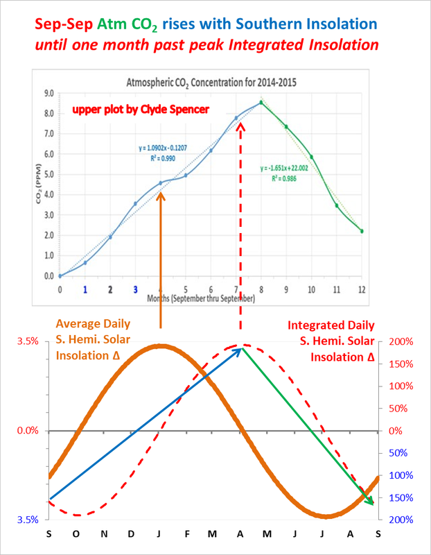
The 10-12 months lag of ML CO2 12mo∆ from monthly HadSST3:
That isn’t what I found in my analysis of the seasonal variations. See Fig. 3 at
https://wattsupwiththat.com/2021/06/11/contribution-of-anthropogenic-co2-emissions-to-changes-in-atmospheric-concentrations/
Nice reference. Thanks.
It pretty much jibes with what my friend has found. ENSO has a large correlation with CO2./
CO2 review number three.
There is poor understanding of the dynamics of CO2 concentrations in the air.
As one example, please refer to the pictures from Clyde’s article, caption “Figures 1a and 1b. CO2 maps from the OCO-2 satellite. (Source: NASA JPL)”
Let us assume that we are seeking locations above the Earth where there are major sinks and major sources. The easy initial assumption is that CO2 in air will show a positive anomaly over sources and a negative one over sinks. The frequent absence of data showing this in satellite observations should have caused pause and a re-examination of the simple starting point.
Let us next assume that roughly, sinks and sources are in balance. Take a simple case of an Earth with one dominant, discrete sink and one dominant, discrete source and think of flow from source to sink. If the sink is very efficient – think of it like a vacuum cleaner sucking away – then yes, there will be a negative anomaly because the CO2 disappears from the air as soon as it gets to the sink.
But what if the sink acts slowly? Like on a scale of years? In our model, this one sink has to consume all the extra material the source is emitting, so we get a build-up of CO2 over the sink, like jets at Heathrow airport on a bad day. Our slow sink model leads to a positive anomaly, NOT what is expected. (Of course, it is affected by the source dynamics, like if LAX is having a slow or fast day as the source.)
Of course, real life is more complicated, with pattern shifts with the seasons and intensity shifts that give those 7 ppm wriggles each year at Mauna Loa. The lesson is, the place-to-place abundance of CO2 in the air is more complicated than is commonly presented in papers. Geoff S
I’ll drink to that!
It is why time series analysis is so important as compared to simple annual averages. Variance in averages can result in a false correlation between variables. Truly, we barely have enough data to adequately analyze some of the cyclical phenomena and their interrelation. Long time resolution proxies have little value in trying to correlate casual relationships.
CO2 review number four.
The work done by the Keelings and associates has been valuable – I do not criticise it. However, users of the Mauna Loa data in particular sometimes use the data without much consideration of its limitations. It is wrong to describe it as the usual atmospheric abundance of CO2 for several reasons. One simple reason is enough to cause concern.
It is often stated that CO2 in air is well mixed. Let us contest this. Imagine a smokestack at an electricity generating station that is powered by fossil fuels. The CO2 that comes out of that concentrated source is assumed to mix will before eventually reaching Mauna Loa for measurement.
But, what if it never gets there? What if trees nearby take up a significant fraction of the CO2 from the air? Why have people assumed so often that it does get to Mauna Loa?
It is easy to envisage many types of sinks that can trap CO2 along the way, leading to concepts of many local micro cells of action, like in a corn field that emits CO2 from photosynthesis cycles part of the day and consumes it at other times. Is this daily cycle largely confined to the corn field and little more distant, or does it really all get into the air to contribute to the well-mixed average?
A great deal of present interpretation of CO2 level in air depend on sorting out the flow mechanisms as to time and place and rate. For example, patterns are different at the Mauna Loa and the South Pole. Geoff S
Actually, as a result of orographic uplift of air masses on the windward side of the island, ocean air has to pass over a considerable amount of vegetation that subtracts CO2 in the daytime and adds CO2 at night.
One wonders that people have not thought to measure it other places as well.
CO2 review number five.
Any interpretation involving measured data has to pay respect to the accuracy and precision of that data. There is little value in claiming evidence for effects that are no more than wandering in the weeds of measurement errors and overall uncertainty.
I gave some views on accuracy to WUWT here –
https://wattsupwiththat.com/2020/05/22/the-global-co2-lockdown-problem/
In summary, it is likely that the usual case applies, namely, that users of data imagine the error are smaller than reality. Geoff S
Clyde,
Great information. It is nice to see data based science related on this site. We need more and more of this as politicians move forward with destroying our fossil fuel based societies.
You got a single down-vote, probably from Tom, who doesn’t agree with you. He seems to have a very large burr under his blanket.
A mass balance on the atmosphere shows that a net emission of about 8 gigatonnes (GT) of CO2 would raise the average CO2 concentration in the atmosphere by 1 ppm. Net emissions means anthropogenic emissions plus natural emissions (including outgassing from oceans) minus absorption by natural sinks (including photosynthesis).
Anthropogenic CO2 emissions are running about 33 GT/year, which would raise the CO2 concentration by about 4.1 ppm/yr if there were no natural sources or sinks. If the actual concentrations are rising at a rate of 1.8 ppm/yr, then natural processes are removing a net 2.3 ppm/yr, or about 18 GT/yr of CO2, from the atmosphere, which amounts to about 56% of anthropogenic emissions.
As noted by Clyde Spencer, the absorption rate of CO2 by photosynthesis varies seasonally (and geographically) due to whether trees are active (in spring and summer) or dormant (late autumn and winter). In tropical areas, vegetation retains its leaves year-round, but since photosynthesis requires water as well as CO2 and sunshine, photosynthesis rates will vary with rainfall.
If Figure 1a above corresponds to October and Figure 1b corresponds to December, there is an interesting pattern in Africa. Southern Africa tends to emit more CO2 in October (early spring there) than in December (near the summer solstice), when trees will be very active. Equatorial west Africa seems to be a net CO2 absorber in October (trees very active) but a net emitter in December (likely the dry season there, when the Equatorial Convergence Zone moves south).
The southern oceans seem to be outgassing more CO2 in October (early spring) than in December (summer solstice). Despite the high insolation there in December (which warms the ocean), photosynthesis by plankton also speeds up, which neutralizes the warming effect.
Photosynthesis actually speeds up with increasing CO2 in the atmosphere, meaning that if anthropogenic CO2 emissions are reversing what would otherwise be a decreasing trend in CO2 in the atmosphere, they are also causing the Earth to be greener and more fertile in food production.
As for net CO2 emissions or absorption in oceans, according to Henry’s Law, CO2 emission rates from the oceans increase with water temperature, but increasing CO2 in the atmosphere tend to promote absorption of CO2 by the oceans. CO2 can also be used by marine organisms to form carbonates for their shells, so the CO2 balance in the oceans can be very complex, and depend also on concentrations of cations dissolved in the oceans, particularly Ca++ and Mg++. The inventory of CO2 in the oceans, either as dissolved gas or as bicarbonate or carbonate ions, is huge compared to the amount in the atmosphere, so that the oceans are the largest source and sink for CO2.
But the CO2 balance on the atmosphere shows that anthropogenic emissions are adding about 33 GT/yr of CO2 to the atmosphere, but the net sum of natural emissions and absorption are removing about 18 GT/yr of CO2 from the atmosphere. It is entirely possible that the current consumption of fossil fuels is removing carbon previously buried miles under the surface and converting what would otherwise be a net decline in CO2 in the atmosphere to a net increase. Anthropogenic CO2 emissions may actually be rendering the Earth more green and fertile, and may actually be preventing or postponing the onset of a new ice age, particularly if the sun may be entering a quiet phase.
Hello,
I am the lead author of the Kieft et al., 2021 study that you cite in your article. Your sentence states:
This is not what we conclude in our paper, nor is 13C even relevant to our findings because we only used it as a chemical tracer in our methods. We do not measure carbon concentration mechanisms, and we certainly do not measure CO2 in any way. You misinterpreted our work.
I strongly request that you rescind my publication from your post and citation list. I do not appreciate having the research I worked hard on to be twisted in this way.
I expect to return here in a few days to see that my work has been removed from this article.
Please contact me if you have further questions.
Brandon Kieft
Dr. Kieft, thank you kindly for your contribution both in your paper and your comment.
I understand that you only used 13C as a tracer and did not measure CO2 in any way.
However, if I understand your work correctly, you’ve shown that there are different kinds of dissolved carbon-containing organic materials (DOC), coming from the lysing and the exudates of various classes of phytoplankton. These are taken up preferentially by other microbial communities which cycle and recycle carbon through the ocean at different rates in different places and times.
Now, we need to couple your most interesting results with the known carbon fractionation properties of phytoplankton, e.g. from Isotopic fractionation of carbon during uptake by phytoplankton across the South Atlantic subtropical convergence:
and from Effect of phytoplankton cell geometry on carbon isotopic fractionation
Combining these two facts, a) that different types of plankton take up different ratios of 13C, and b) your finding that the carbon from different types of plankton moves via different metabolic pathways through different microbial communities, it would seem logical that in some areas at some times, 13C will be either concentrated or dispersed …
Am I correct in this conclusion, and if not, why not?
Many thanks,
w.
I’m surprised at your strong reaction to me saying,
I didn’t say that you made the claim. It is my interpretation of the statements (as shown below) from the article cited.
I may well have misunderstood key points of the paper inasmuch as the subject matter is outside my areas of expertise; however, considering that you make statements such as,
1) “We observed significant 13C labeling of the coastal microbial community after only 15 h of 20 °C incubation with all four labeled substrates …; however, the two phytoplankton species (diatom or cyanobacteria) and two cell fractions (lysate or exudate) did not elicit the same frequency or magnitude of 13C assimilation into heterotroph biomass.”
And,
2) “We propose that this observation supports two possible conclusions. First, Pelagibacteraceae cells are synthesizing more proteins in the substrate-addition treatments compared to the no-substrate control, but they are not efficiently using 13C-labeled resources for anabolism and are instead relying on existing (un-labeled) substrates for biomass synthesis.”
And,
3) “While our data cannot definitively rule out this zero-sum-game scenario, our results do show that most other dominant taxa did exhibit high 13C-enrichment and activity, undermining the latter option that other abundant taxa were decreasing in biomass relative to the Pelagibacteraceae. Furthermore, there is precedence for a mechanism of metabolic partitioning that supports the former option describing a low carbon use efficiency model and that may be worth considering for future studies of Pelagibacteraceae physiology.”
Finally,
4) “Low-abundance taxonomic groups showed similarly low levels of enrichment in substrate treatments on the time scale we used in our experiments. Given that we observed relatively little 13C assimilation by low-abundance groups, their contribution to ecosystem-scale carbon cycling appears to be proportional to their low representation.”
It is commonly known that plants have a preference for the light 12C carbon isotope. I would be surprised if other organisms didn’t have similar preferences, and that it didn’t vary with the species, depending on what they typically fed on, and perhaps even what the carbon ratios were when the organism first evolved.
When I looked for evidence, I came across your paper. I recognize that you did not intend to demonstrate isotopic fractionation in your research and might be a little surprised that you uncovered implicit evidence for it. Just because you didn’t specifically look for isotopic fractionation in bacteria doesn’t mean that you didn’t inadvertently provide evidence for it.
I think that we should let the readers decide if I erred in citing your work to support my conjecture that isotopic carbon fractionation may occur when marine bacteria decompose algal blooms. Thank you for the opportunity to expand on the single sentence in my article.
The m&m analogy would have been better if each guest had brought ones which had been treated with radioactive trace elements of varying half-lives. Atmospheric CO2 contains istotopes of carbon (C12, C13, and C14). The source of m&m’s cannot be differentiated as we can with CO2 based on its isotopic makeup. Fossil CO2 is completed depleted of C14, for instance. This affects the C12:C14 ratio in atmospheric CO2.
The above statement is clearly wrong or highly misleading, or it is a truism. It would be impossible to say with complete certainty that there is nothing but anthropogenic CO2 emissions affecting the global atmospheric CO2 concentration. The real argument is that the increase is primarily due to anthropogenic CO2 emissions, for which there is ample empirical evidence.
Regarding WE’s comment above, doesn’t it matter a great deal whether 13C is being concentrated or dispersed? This just boils down to idle speculation. Citing the BK, et al paper leaves the casual reader with the impression that there is something in it which strongly supports Clyde’s argument, which there isn’t.
Clyde’s post makes no mention of 14C. How can he dismiss completely the evidence for an anthropogenic source for the CO2 increase without addressing this?
Perhaps that is all that you are capable of seeing. However, someone with more vision would immediately recognize that it exposes an area that hasn’t been explored sufficiently to be able to say whether the impact is negligible or important. It reinforces the position that the science is not settled.
The article is almost 2700 words, which is large for this forum. Some things have to be left out — even when writing a book. I think that your complaints are little more than whining.
However, I will point out that CO2 and methane released from the tundra are deficient in 14C, as is CO2 from melting Greenland and Antarctic ice. CO2 associated with upwelling of deep ocean water is about 1,000 years old and is deficient in 14C. Limestone exposures throughout the world are millions of years old, and are completely depleted in 14C. Therefore, when they are dissolved by acidic rain and organic acids (e.g. humic acid), the released CO2 contains no 14C, other than what was in the rain. Although relatively small in volume, volcanic CO2 is also depleted of 14C. Most of these sources are not taken into consideration when calculations are performed on the atmospheric 14C ratio. Therefore, I would judge that the 14C ‘evidence’ used to support the view that the atmosphere is changing because of anthropogenic activities is less than rigorous.
I think that readers are also entitled to know, if the current upward trend in CO2 is not due to anthropogenic CO2 emissions, and is instead due to isotopic fractionation in the biosphere or some other phenomenon, what has caused the change? Is there an argument that isotopic fractionation in the biosphere is somehow different than it was 100 years ago? What caused that?
May I recommend this paper by Keeling et al (2017):
Atmospheric evidence for a global secular increase in carbon isotopic discrimination of land photosynthesis, Proceedings of the National Academy of Sciences, 114(39), 10361-10366. DOI: 10.1073/pnas.1619240114.
https://www.pnas.org/content/pnas/114/39/10361.full.pdf
They concluded (as recently as 2017!) that:
“Using updated records, we show that no plausible combination of sources and sinks of CO2 from fossil fuel, land, and oceans can explain the observed 13C-Suess effect unless an increase has occurred in the 13C/12C isotopic discrimination of land photosynthesis”.
They do not claim that the change in isotopic fractionation (disequilibrium) is the cause of CO2 growth, but they do claim that it is is necessary to explain 30% of the enormous mis-match in isotopic mass balance terms between the observed decline in atmospheric δ13C and the theoretical value of adding estimated CO2 emissions from fossil fuels (see table S5).
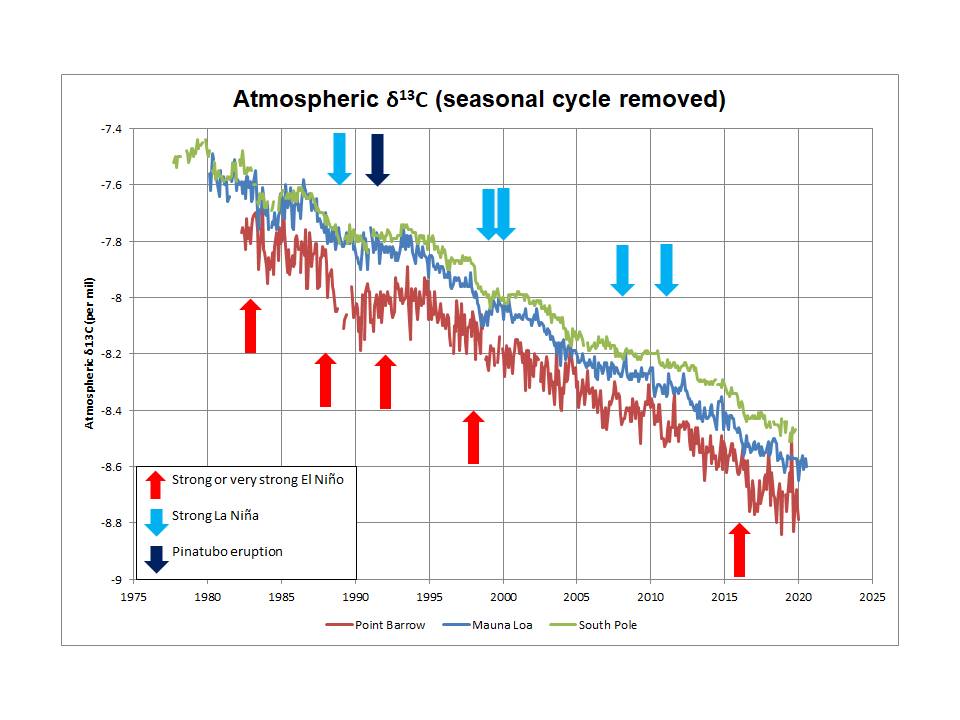
They appear to have failed to recognize a critical constraint on models which is that the decline in atmospheric δ13C reflects a net value of -13 per mil for the additional atmospheric CO2 (averaged over a few years to remove the effect of fluctuations due to ENSO and Pinatubo).
More importantly, in my view, is that they do not attempt to match the inter-annual variations in δ13C – these changes are extremely important in understanding the behavior of CO2 in terms of sources and sinks since they reflect, in part at least, the impact of ENSO on atmospheric δ13C.
See: van der Velde et al (2013): Biosphere model simulations of interannual variability in terrestrial 13C/12C exchange, Global Biogeochem. Cycles, 27, 637–649, doi:10.1002/gbc.20048.
https://agupubs.onlinelibrary.wiley.com/doi/full/10.1002/gbc.20048
They note that: “But the year-to-year variability in the isotopic disequilibrium flux is much lower (1σ=±1.5 PgC per mil yr−1) than required (±12.5 PgC per mil yr−1) to match atmospheric observations, under the common assumption of low variability in net ocean CO2 fluxes”.
Bottom line: despite the constant claims that the observed decline in atmospheric δ13C is due to the addition of anthropogenic emissions, there are currently (to my knowledge) no published models that are able to replicate the observed behavior, especially the inter-annual variations, but also the evidence from the Law Dome ice core data (which also shows an average δ13C of -13 per mil for all additional atmospheric CO2 since around 1760).
Thanks for those insights, Jim. I would have to go back and read more to fully appreciate what you’ve written. But on first glance, I’ll note that this goes way, way beyond the silly (as I see it) arguments of Clyde Spencer. Clyde was not merely casting doubt on the validity of attributing all CO2 increase to fossil fuel combustion, he was rejecting that argument out of hand. Secondly, he, and you, never discuss 14C, the declining presence of which, suggests strongly a fossil carbon source.
I do not discuss 14C here mainly because I have focused most of my analysis on the stable isotopes of 12C and 13C to which mass balance applies. As such, this permits investigation and meaningful conclusions about data relationships based solely on observations, which then provide important constraints on possible physical explanations (models).
The above, from the reference you cited makes complete sense to me, As vegetation globally responds to the increase in CO2, it makes sense that the atmospheric CO2 balance should take this into account, and it should be an area of study. However, I believe some feel this has been accounted for already:
Global Monitoring Laboratory – Carbon Cycle Greenhouse Gases (noaa.gov)
Please let me know if I’m missing a key point.
See my comment above at December 18, 2021 10:19 am
I am out of time, so will respond more fully tomorrow. In the meantime, two key points are that the average δ13C of additional atmospheric CO2, possibly since 1760, has been constant, and there appears to be no current published models that are able to explain the inter-annual variations in atmospheric δ13C.
I apologize for the length of this comment, but the underlying basis for one my key points has not been published by others, as far as I know, so I cannot simply link to more detailed articles elsewhere. I have sub-divided the text in several parts because of the length. Very happy to be corrected, provided such points are supported by actual numbers.
Part 1
First, a few introductory remarks,
Unless otherwise stated, the monthly data used in the following comments and plots were downloaded from the site of the Scripps CO2 program and are either the ‘raw’ monthly values (i.e. including the seasonal cycle) or those with the seasonal cycle removed by Scripps. Missing data are shown as data gaps herein, although in-filled datasets are also available from Scripps. This also applies to the Keeling plot I showed above; my apologies for forgetting to provide the source of the data used in that plot (which I created).
I am not about to argue how much or how little additional atmospheric CO2 is from anthropogenic emissions. This requires a number of assumptions or estimates based on models which are, by definition non-unique possible physical explanations of what we observe. We cannot prove that a specific model is correct. We can, however, prove that a model is invalid if it deviates from observations, including known data relationships, which must constrain the model. It is establishing these known data relationships that I focus on.
In case there is anyone still reading here who are not familiar with the δ13C nomenclature as applied to CO2, here is a brief explanation. Put simply, the δ13C of a CO2 sample is the difference between the measured 13C/12C ratio and the 13C/12C ratio of a fixed standard, expressed in per mil terms. Thus, a negative δ13C means that the sample has a lower 13C/12C ratio than the standard. The units of ‘per mil’ mean per thousand, so exactly the same as if expressed as a percentage (per hundred) but multiplied by 10. So, for example, a δ13C of -13 per mil means that the sample has a 13C/12C ratio that is 1.3% lower than the 13C/12C ratio of the standard.
Above, I showed a Keeling plot for the South Pole observations; this is a plot of pairs of measurements of δ13C and the reciprocal of CO2 and is based on isotopic mass balance equations. The paper by Kőhler et al (2006) provides a fairly good summary of the basis for such plots, including the relevant equations, where a linear relationship indicates a constant value for the δ13C of the incremental CO2 and the intercept gives the δ13C value. The authors highlight two caveats with respect to the application of Keeling plots:
“There are two basic assumptions underlying the Keeling plot method: (1) The system consists of only two reservoirs. (2) The isotopic ratio of the carbon in the added reservoir [source of the additional CO2] does not change during the time of observation”.
Point 2 is certainly true, but point 1 is not strictly a requirement. There could be more than two reservoirs (sources/sinks) but the method will still work provided that point 2 is maintained. Of course, the probability of a multi-reservoir source/sink system, with varying fluxes with different δ13C contents and fractionation characteristics, having a constant net δ13C over time would be extremely small. Conversely, if the Keeling plot does show a strong linear relationship, this can only occur if the net δ13C of CO2 being added to the recipient reservoir (the atmosphere) is not changing significantly over time. This is precisely what the observations show, so either we have an amazing coincidence or we have a dominant source which is not changing over time.
I think that the two most important points that you make here are:
1) “the average δ13C of additional atmospheric CO2, possibly since 1760, has been constant, and there appears to be no current published models that are able to explain the inter-annual variations in atmospheric δ13C.”
2) “… this can only occur if the net δ13C of CO2 being added to the recipient reservoir (the atmosphere) is not changing significantly over time.” Clearly, anthro’ is changing!
Yes, Clyde, I agree.
If we refer to the model of Keeling et al (2017), we find that it is based on five different inputs to the predicted behavior of atmospheric δ13C – refer to Table S5 in the appendix, accessible from the paper itself. Let me know if you have trouble accessing it. So their model requires the combination of these five different source/sink interactions to maintain a consistent net δ13C flux of -13 per mil over time, which seems rather unlikely to me. Indeed, the model failed to do this before they added the new variable.
In isotopic mass balance terms, simply adding fossil fuels to the atmosphere leads to huge decrease in δ13C, much larger than actually seen in the observations (almost eight times too much in isotopic mass balance terms). So the model needs to offset that with source/sink interactions which ‘correct’ that mismatch: 20% of the correction is derived from uptake of CO2 by the oceans and the land, as required by the model to achieve a mass balance of CO2, but 80% is attributed to ocean and land disequilibrium fluxes which occur by ongoing exchanges in CO2 between sources and sinks (due to differential fractionation) without adding or removing CO2.
These disequilibrium fluxes seem to me to be rather poorly constrained and yet are crucial (in the model) to obtaining a match with the observations.
I will respond separately regarding the inter-annual fluctuations.
Part 2
Let’s look at the simple mass balance of 13C first (equation 4 in the Kőhler et al paper referenced above). This provides a long term average net δ13C of the incremental CO2 without any need to consider sources/sinks separately or the fact that increases in atmospheric CO2 have not been linear since the start of CO2 growth. If we take the ‘initial’ values of CO2 and δ13C respectively as 280 ppmv and -6.4 per mil at 1760 or thereabouts based on Law Dome ice core data, and direct atmospheric measurements in January 1980 as 336 ppmv and -7.50 per mil and in January 2019 as 406 and -8.44 per mil, we can determine the average δ13C between those dates as follows:
From 1760 to 1980:
(-7.50*336 + 6.4*280)/(336-280) = -13 per mil
From 1980 to 2019:
(-8.44*406 + 7.50*336)/(406-336) = -13.0 per mil
Incidentally, the above equation contains a very small (insignificant) approximation since it is based on multiplying CO2 and δ13C (effectively the 13C/12C ratio) to get the quantity of 13C. It should be using 12CO2 rather than total (measured) CO2. However, since 12CO2 is 98.9% of total CO2 this has no material effect and is widely used in the literature (and is easily checked by converting δ13C back to the actual 13C/12C ratio and correcting for the difference).
The above calculated long-term averages are valuable since they require only mass balance calculations to confirm them. We do not need to understand anything about sources and sinks, because we are looking solely at the net effect. However, we are (or should be) interested in how these averages may have deviated over time and hence we need to look at the linearity (or otherwise) of the relevant Keeling plots.
First, the Keeling plot of the Law Dome ice core data is shown in the Kőhler et al paper referenced above in Figure 1. The intercept is -13.1 per mil and the r-squared is 0.96. The South Pole plot shown earlier gives an intercept of -13.0 per mil, r-squared of 0.99. Keeling plots (seasonal cycle removed) for Mauna Loa and Point Barrow give intercepts of -13.4 per mil and -13.2 per mil, respectively, with r-squared values of 0.98 and 0.96.
Part 3
Moving on to the Keeling et al (2017) paper referenced previously, their model was initiated in 1765 using CO2 of 278 ppmv and δ13C of -6.4 per mil. They then used an average of the observations from Mauna Loa and South Pole, with the seasonal cycle removed, so we need to do the same for selecting the appropriate CO2 values (though averaging two sets of observations is not something I would normally choose to do).
We can see in their Figure 1A that the “standard model run” failed to match both the starting point of δ13C observations in the late 1970s and the gradient of δ13C decline through to end of 2014. So how would the observed data relationship (my ‘model’) of a constant value of -13 per mil have performed?
February 1980 was the first month for which both sites had CO2 and δ13C observations, giving an average of 337 ppmv and -7.52 per mil. Based on their graph, their standard model run predicted about -7.75 per mil. My ‘model’ predicts -7.56 per mil, much closer to the measured value of -7.52.
(278*-6.4 + (337-278)*-13)/337 = -7.56.
December 2013 was the last month used in the Keeling et al (2017) model, where observations gave an average of 396 ppmv and -8.36 per mil. Based on their graph, their standard model run predicted about -8.78 per mil. My ‘model’ predicts -8.37 per mil, again much closer to the measured value of -8.36 per mil. Note that my ‘model’ estimate is based solely on the values used by Keeling et al for 1765, the measured CO2 in December 2013, and an assumption of a constant δ13C of -13 per mil.
(278*-6.4 + (396-278)*-13)/396 = -8.37.
The main point of this exercise was to demonstrate that using a constant δ13C for incremental atmospheric CO2, even going back as far as 1765, provides a much better match to observations than the “standard model run” of a recent and highly sophisticated mass balance model constructed by experts. The value of that constant δ13C was derived entirely from observations and did not require any assumptions about sources and sinks. The linearity of the Keeling plots demonstrated the validity of their interpretation, and this was separately confirmed by application of simple mass balance calculations over extended periods, again without any consideration of sources and sinks.
The failure of the Keeling et al (2017) standard model run to match observations (prior to adding further to its complexity by invoking variability in a previously fixed parameter) proves that the model in that form was invalid. The revision to their model was designed to derive a closer match to the observed δ13C decline rate and this was achieved by adding a CO2-dependent nature to a parameter that was previously fixed. This would appear to be in conflict with the known data relationship of a constant δ13C of the incremental CO2. This does not mean the new version of the model is necessarily incorrect; however, it should be of some concern that it is necessary to add further complexity in order to match what is apparently a very simple relationship.
I will have to address the other key point of δ13C behavior during ENSO events another day. This was not addressed by Keeling et al (2017) and potentially has a direct bearing on the validity of any explanatory model of atmospheric growth in CO2.
Might it be that the unexplained atmospheric δ13C interannual variations are related to weather and El Nino cycles affecting temperature?
Yes, I think ENSO could be a key element of the inter-annual variations in atmospheric δ13C. After all, it is well established that ENSO drives such variations in CO2 growth rate, but the key question is this: does the net δ13C content of the incremental CO2 change during such events (and Pinatubo as well).
First, I draw your attention to the following plot which I generated fairly recently:
We can glean several key points.
I have prepared a simple to model to evaluate this point. The numbers used in the model for δ13C are not meant to be definitive, but they do need to be directionally correct to explain the observations.
Figure 1 shows the observations (seasonal cycle removed) for Mauna Loa for the El Niño of 1997-1998 and subsequent La Niña. The increased rate of growth in atmospheric CO2 is clearly evident, starting in late 1997 and finishing in mid-1998. Atmospheric δ13C shows a rapid drop in late 1997 through to mid 1998, which is synchronous with the CO2 rate changes.
Figure 2 shows the same δ13C data in red, while the green data is calculated from the CO2 data shown on Figure 1 by assuming that the CO2 trend reflects a constant net δ13C content of -13 per mil for the incremental CO2. While it shows an increase in the rate of decline of atmospheric δ13C as expected, the drop is nowhere close to the observed change.
The basis for Figures 3 and 4 are stated on the figures. In Figure 4, the model δ13C was changed to -26 per mil from late 1997 to mid 1998 during El Niño and then to 0 per mil until late 1999.
So, it would appear that higher CO2 growth rates broadly correspond to a lower net δ13C content of CO2 than the average of -13 per mil, while lower CO2 growth rates associated with La Niña events (and Pinatubo as well) coincide with a higher net δ13C content of CO2 than average, generally closer to the then current atmospheric δ13C level and possible even higher on occasion.
Looking again at this Keeling plot below, changes in net δ13C content (which is seen in the intercept of a linear fit to the data) appear through time and show periods of lower than average δ13C content of the incremental atmospheric CO2 (steeper gradient) offset from time to time by short periods of higher than average δ13C content.
I would speculate, therefore, that the reason that there are no current models that explain the inter-annual variations in atmospheric δ13C is that the models do not capture changes in the net δ13C content of CO2 during major ENSO (and volcanic) events. I would certainly welcome comments and alternative explanations of observed data relationships.
“I think that readers are also entitled to know” that you obviously don’t understand the issue! I never claimed that isotopic fractionation is responsible for the upward trend in CO2. My argument is that the evidence, based on isotopic ratios, used to support the claim that anthropogenic CO2 sources are solely responsible for the upward trend, does not take into account other possible mechanisms for changing the isotopic ratio. Therefore, it amounts to Cherry Picking.
Measurements after the atmospheric nuclear bomb tests showed carbon in CO2 has a 16 year half life in the atmosphere.
residence time = half life / (nat-log2)
= half life / 0.693 or half life x 1.44
= 23 years.
That’s the beginning and the end of CO2 kinetics in the atmosphere.
Talk of recycling and e-folding time and compartments etc. is just wishful bluster aimed at extending the CO2 residence time toward infinity, to meet political needs.
The assertion is made that it is assumed that only anthropogenic emissions are responsible for the increase atmospheric CO2 level. I don’t know of any credible source that insists that it’s only CO2 and cannot be anything else, but I would await a citation on that. I do think that it is widely believed that anthropogenic emissions are the predominant reason for the increase. To support the claim of no empirical evidence, the author cites the failure of the 2020 reduction in global annual anthropogenic CO2 emissions to alter the seasonal variation in the Keeling curve. If one does the calculations, the 9 ppm annual runup is equivalent to 7×10^13 Kg of CO2. The 5% decrease for the year 2020 is equivalent to 1.7×10^12 Kg of CO2. The seasonal variation is roughly 40 times greater than the impact of the 2020 decline. It is possible that the change in anthropogenic emissions gets washed out or overwhelmed by natural changes. I think it is a fair point, but in order to make any more of it, a more detailed analysis might be required. The author has also emphasized that the total flux of CO2 in and out of the atmosphere is very much greater than the influx due to anthropogenic emissions. I think this supports the notion that the 5% drop of the 4% (CO2 emissions as a percent of total flux) is de minimis, and therefore might not show up in the short term. I assume someone will check my calculations.