Clyde Spencer
2021
PARTY TIME
Imagine that someone decides to throw a theme party and the theme they choose is ‘blue.’ They invite 10 of their friends and ask each of them to bring a plastic baggie filled with blue M&Ms™ candies. When the guests arrive, they empty their baggies into an empty punchbowl. The host(ess) places the filled bowl on the hors d’oeuvres table. Assuming that each of the guests brings on average about 100 pieces, there will be about 1,000 pieces total. Throughout the evening, the guests partake sparingly of the contents of the punchbowl (the host(ess) abstains.). At the end of the evening, there are still some candy pieces left. As they are leaving, one of the guests claims them, boldly stating that there are about half as many candy pieces as he brought, and they must therefore be the same ones he brought, despite having brought noticeably fewer pieces of candy than the others had! Other than being a bit boorish, what can we conclude about the claim?
Strictly speaking, we are dealing with a situation of sampling without replacement, which means that the probability of drawing a piece of candy contributed by any person varies over time, depending on how many of a particular person’s contribution remains after withdrawals. Unfortunately, we don’t have that information. I’m assuming, for the sake of illustration, that approximately equal numbers of candy from all the guests are drawn, and that the total number of pieces of candy is large enough that, at least initially, there is a negligible change in the ratio of the pieces drawn to the number remaining. Therefore, the probability remains approximately constant until we get below 10 pieces. Thus, the following reliance on the initial probability. As is the practice in climatology, I’m going to ignore probability uncertainties and their propagation. I’ll just work with orders of magnitude.
If there were only one piece of candy left, we could trivially conclude that there was 100% probability that one person brought it. However, who? Probably the first person to arrive and put their candy in the bowl if the contents hadn’t been mixed. FILO – First In, Last Out! Alternatively, more probably, the person who brought the most candy, if the contents are well mixed. However, in the absence of information on the quantity and order of the candy placed in the bowl, the best we can probably do, assuming that everyone brought approximately the same number of pieces of candy, is to say that the single remaining piece has about a 1:10 chance of belonging to a particular person, or 0.1. Although, that doesn’t allow us to determine who that person is.
Things get a little more interesting and complicated if there are two pieces of candy left over. What is the chance that the same person brought both pieces? The probability of a sequence of events is the product of the probabilities of each event. That probability is about 0.1 x 0.1 or 0.01, in the well-mixed case, which I will assume. What if there are five pieces left? The probability that the same person brought all five remaining pieces would be about 0.1 raised to the 5th power, or 0.15 ≈ 10-5. It should be obvious that attribution of source rapidly becomes uncertain as the number of sources increases and the number of events (pieces of candy) increases! Therefore, it becomes very unlikely that the same person brought all of the remaining pieces. That is, having a large number of pieces of candy left over, all from the same person is highly improbable. However, the probability increases to 1 as a limit as the number of pieces of candy declines to 1.
ANALOGY TIME
In the above story, the punchbowl represents the tropospheric atmosphere, the contributed blue M&Ms the annual flux of well-mixed CO2 that is added over the Winter, and the candy consumed represents the annual flux of CO2 that is captured by the global sinks, principally during the Summer. The number of pieces of candy remaining at the end of the party represents the annual net increase in CO2. It is claimed commonly that, because the atmospheric concentration of CO2 is increasing annually by an amount that is almost half the estimated anthropogenic emissions, humans are solely responsible for the increase in atmospheric CO2, and ergo, eliminating anthropogenic emissions will stop the rise of CO2 and therefore stop the rise in temperature of the globe.
One problem with the assumption that only anthropogenic emissions are responsible for the annual increase in CO2 is that there is no empirical evidence for it. The decline in anthropogenic emissions during the height of the COVID pandemic did not result in any measureable decline in the total increase during 2020, or rate of increase for any of the months; nor was the decline faster than typical. I have discussed this in detail here: https://wattsupwiththat.com/2021/06/11/contribution-of-anthropogenic-co2-emissions-to-changes-in-atmospheric-concentrations/
Summarizing the above linked article, the atmospheric CO2 concentration varies seasonally. It increases about 8 PPMv from Oct thru May, and decreases about 6 PPMv from June thru Sept. During the ramp-up phase, Fall thru early-Spring, photosynthesis is significantly reduced and the net change is an increase in atmospheric CO2 concentration. However, during April of 2020, there was a pandemic-induced decline of about 18% in anthropogenic CO2, but there was no observable change in the rate of increase; the curve essentially looked like the previous year. Similarly, the maximum concentration reached in May was virtually the same as in 2018-2019, despite there being reduced estimated anthropogenic CO2 emissions, December 2019 through May 2020.
The anthropogenic sources of CO2, not all of which are from burning fossil fuels, only amount to about 4% of the total CO2 flux in the Carbon Cycle, which strongly suggests that the small flux of anthropogenic CO2 is dwarfed by the biogenic sources and outgassing from warming water, leading to a negligible residual anthropogenic accumulation in the atmosphere.
All CO2 is partitioned into the various sinks (air, water, terrestrial plants, phytoplankton) in proportion to the fractional abundance compared to the annual total. The sinks cannot tell the difference between CO2 sourced from fossil fuels, plant respiration, or bacterial decomposition! That is, if all fossil fuel emissions were to magically cease tomorrow, we could only expect to see <4% decline in the rate of atmospheric CO2 concentration growth, not the 50% we are being told to expect.
The problem is that sources and sinks are more sensitive to the abundance of CO2 (partial pressure) than other differences such as the atomic weight of the CO2 molecules. Therefore, the sources can’t significantly differentiate between anthropogenic and natural sources, such as biogenic CO2 or ocean outgassing. The same is true for sinks, with the notable exception of photosynthetic organisms showing a slight preference for light CO2 molecules with a 12C isotope. That is the point of the little story above about the M&Ms. That is, if the person claiming the remaining pieces of candy had not brought any, there would still probably be some candy remaining, although it obviously could not have been his.
Another way of looking at this issue is that, for a first-order approximation ignoring isotopic fractionation, the sinks should extract CO2 out of the atmosphere in direct proportion to the relative abundance of the source CO2. That is, if there is a net annual gain of 2 or 3 PPM, almost all of that has to be from the sources with the greatest abundance – oceanic out-gassing and biogenic respiration. The same argument about the trivial contribution from volcanic activity applies equally to anthropogenic emissions.
Most of the claimed supporting evidence for anthropogenic CO2 concentrating in the atmosphere is based on changes in the isotopic carbon proportions. The argument is that fossil fuels have a small deficit of 13C and the measured increase in the relative proportion of atmospheric 12C must therefore be from CO2 derived from fossil fuels. The situation is more complex than suggested because recent work (Kieft, et al., 2021) has shown that bacterial recycling of dissolved organic matter in the oceans may concentrate the 13C isotope!
During nighttime, plants respire CO2. Dormant deciduous trees still respire (during Winter) through their roots. However, evergreen trees in boreal forests respire more because they retain their needles. I would expect this respiration, which contributes to the Winter CO2 ramp-up to be deficient in 13C.
Another flaw in the isotope defense is that there should be a preference for light (12C-rich) CO2 outgassing from the ocean surface because it takes less energy for wind to strip it out than for the heavier molecules. I’m unaware of anyone having taken this into consideration when defending the claim of the increase in atmospheric CO2 being the result of anthropogenic emissions, despite some early work having been done (Doctor, et al., 2008) with freshwater. Additionally, Mayorga et al. (2012) show that isotopic fractionation occurs between the dissolved carbon species carbonic acid, aqueous bicarbonate, and aqueous carbonate, during conversion between species, with pH change, as well as with outgassing. Earlier work by Wanninkhof (1985) left some questions unanswered, but stated:
“A box model of Keeling et al. (1980) shows a difference in δ13C change in the atmosphere from 1956 to 1978 of 0.15 ‰ depending on whether an air-seawater fractionation constant of -14 ‰ or 0 ‰ is used. This is quite significant if we consider that the total δ13C change in the atmosphere for the past 100 years is about -I ‰, based on tree ring data (Peng et al., 1983).”
EVIDENCE TIME
Since the launching, in late-2014, of the Orbiting Carbon Observatory-2 (OCO-2) satellite, I have seen many CO2 maps. I was unable to find most of them with a general online search. They were not available at the NASA JPL OCO-2 website. The entire archive apparently has been reprocessed, but all that I was able to find was 2015 through 2017 data. At least one video was deleted (the link is not functioning) from the NASA JPL OCO-2 website. The recent maps are not as user friendly as the original graphics released to the public. In searching for suitable OCO-2 CO2 maps, I was impressed by two things: 1) How difficult it was to find previously published maps, and 2) How much variation there was in the few available maps.
Despite being characterized as “well-mixed,” within the limits of quantitative resolution, CO2 varies considerably in concentration, location, and with the seasons. The earliest CO2 map from the OCO-2 satellite is probably the most useful for this discussion because it shows the distribution of concentrations for a 5-week period during the beginning (low point) of the seasonal ramp-up phase for the northern hemisphere (NH).
Figure 1a (below) is the first release of OCO-2 data at the 2014 American Geophysical Union meeting. It appears that the major sources are on land, such as the Amazon Basin and southern Africa, with secondary sources from outgassing in the oceans in an Equatorial belt. These are not regions of either high population density or concentrated industrial activity.
Following that up with another map, Figure 1b, made with data from about two months later, shows how much the location of the major sources changed in just a month in the early NH ramp-up phase. None of the red and little of the yellow that is shown is from cars or factories. Clearly, natural biogenic sources associated with decaying detritus lying on the ground, and evergreen tree respiration, particularly in the boreal forests of North America and Siberia, dominate the Northern Hemisphere sources. The outgassing from the tropical oceans is gone, perhaps because it is early-Winter and the surfaces waters have cooled. It appears that there is still a band of northerly CO2 source from the ocean; however, it may be the result of dead, decomposing phytoplankton still near the surface.


The curve for the 2014-2015 CO2 ramp-up phase (See Figure 2, below.) is typical for the last 30-years, albeit the maximum in May is lower than in recent years. However, the following year was an El Niño year and the May high was typical of recent years. This suggests temperature controlling the CO2 concentration.
Note that the deviations from the linear regression lines recur in most years and are not just random variations in interannual variance.
Fundamentally, it appears that the increase in CO2, as exhibited during the Fall-Spring ramp-up phase, is not being matched by the drawdown phase in Summer, despite the slope of the Summer curve being steeper.

The months marked in blue (1 & 3) correspond to the two maps in Fig. 1a and 1b.
SUMMARY TIME (and the living is easy)
The major sources of CO2 are not spatially associated with high population densities or industrial activity during the seasonal ramp-up phase, with the possible exception of China.
It is improbable that more than a small fraction of the annual anthropogenic emissions remain in the atmosphere because its proportion of total source annual-flux is <4%. The stated fact that the annual increase in atmospheric concentration of CO2 is about one-half the anthropogenic emissions is probably a spurious correlation.
The accounting for the change in atmospheric CO2 isotopic composition resulting from fossil fuel emissions is not rigorous for all the potential sources of isotopic fractionation.
An alternative interpretation for the current paradigm is that, against a background of relatively constant anthropogenic emissions, the warming Earth forces an increase in ocean out-gassing and biogenic emissions during the seasonal CO2 ramp-up phase. During the drawdown phase, the warming high-latitude waters are less effective at capturing the CO2 in the atmosphere. Also, during the drawdown phase, the increased CO2 in the atmosphere results in increased growth of vegetation and photosynthetic plankton; however, the increase is only sufficient to capture an amount of CO2 that is equivalent to about half of the annual anthropogenic emissions. Therefore, in the absence of anthropogenic emissions, one might expect the growth in atmospheric CO2 to be 96% of the current total annual CO2 flux. The average annual net growth in atmospheric CO2 is about 1.8 PPM over the last 30 years. Therefore, one could expect that in the absence of anthropogenic CO2, the annual increase might be about 1.7 PPM. However, because fossil fuels only represent about 95% of anthropogenic emissions, and it is impractical to stop making cement and quit using CO2 as an industrial feedstock, the net annual gain would be somewhat greater than 1.7 PPM. Thus, even draconian emission reductions of anthropogenic CO2 cannot be expected to have more than negligible effect!
It is a common alarmist refrain that when temperatures go down, it is weather; however, when temperatures go up, they call it climate. There is a similar situation with atmospheric CO2. When atmospheric concentrations go up, it is claimed to be solely the result of increasing anthropogenic emissions. When anthropogenic emissions go down, we are told that natural variability masks the expected decrease.
CITATION TIME
Brandon Kieft, Zhou Li, Samuel Bryson, Robert L. Hettich, Chongle Pan, Xavier Mayali, Ryan S. Mueller (2021). Phytoplankton exudates and lysates support distinct microbial consortia with specialized metabolic and ecophysiological traits. Proceedings of the National Academy of Sciences Oct 2021, 118 (41) e2101178118; DOI: 10.1073/pnas.2101178118 https://www.pnas.org/content/pnas/118/41/e2101178118.full.pdf
Doctor, D. H., Kendall, C., Sebestyen, S. D., Shanley, J. B., Ohte, N., & Boyer, E. W. (2008). Carbon isotope fractionation of dissolved inorganic carbon (DIC) due to outgassing of carbon dioxide from a headwater stream. Hydrological Processes, 22(14), 2410-2423. https://doi.org/10.1002/hyp.6833
Mayorga, E., A.K. Aufdenkampe, C.A. Masiello, A.V. Krusche, J.I. Hedges, P.D. Quay, J.E. Richey, and T.A. Brown. (2012). LBA-ECO CD-06 Isotopic Composition of Carbon Fractions, Amazon Basin River Water. Data set. Available on-line [http://daac.ornl.gov ] from Oak Ridge National Laboratory Distributed Active Archive Center, Oak Ridge, Tennessee, U.S.A. http://dx.doi.org/10.3334/ORNLDAAC/1120
Wanninkhof, Rik (1985) Kinetic fractionation of the carbon isotopes 13C and 12C
during transfer of CO2 from air to seawater, Tellus B: Chemical and Physical Meteorology, 37:3,
128-135, DOI: 10.3402/tellusb.v37i3.15008 https://www.tandfonline.com/doi/pdf/10.3402/tellusb.v37i3.15008
Dr. Happer shows that a doubling of CO2 will have no effect as he says this is saturated.
I wonder what if CO2 was cut to 50%.
This slide has been shown at WUWT often :
The human contribution to the annual CO2 outgassing is less than 5% of the total. To make wild assumptions about the whole EARTH doubling Co2 emissions is simply preposterous. that simply is not within the slightest possibility. If the HUMAN contribution was doubled, we would probably not notice a change in climate. Likewise, if ALL human emissions were halted, the climate would not take notice. Why? Because natural emissions vary by about 15% annually, and we don’t notice.
And really we would only know by sampling since ,due to saturation, there would be no temperature rise caused by CO2, regardless of the source …so obviously that leads to a different causal relationship with the rise in temperature.
Because of the fixation with CO 2 there seems to be very little research towards alternate causes
That chart doesn’t really help an anti-alarmist viewpoint very much. It shows a difference of 3 W/sq.M. for a CO2 doubling. That is about double the 1.6 W/sq.M that the IPCC says is the net present anthropogenic contribution for 280 ppm to 400 ppm…so to an alarmist, it is “confirmation”…
But instead of 800 ppm, try 3200 ppm in Modtran, which is about 25 times the amount of “anthro”CO2 increase since civilization began, or 50 times if you assume oceans absorb half….and you will come to the conclusion that the resultant temperature increase versus the current rate of fossil fuel depletion is not worth any effort other than to not waste fuel. Fossil fuels will run out (in the sense of requiring more energy to exploit than they can produce) and humanity will have to go to nuclear power before we hit 1000 ppm CO2….
And this chart doesn’t see the significance of energy in/output.
http://homework.uoregon.edu/pub/class/es202/GRL/ghgfig1.PNG
Note although the curves are drawn with the same size, they have different scales.
In is at 2,000 and out is at 8.
Increase per his reckoning would prevent more from getting to the surface.
The only real effects CO2 has on the atmosphere is to change the specific heat of dry air and to increase the mass. This would alter the lapse rate also.
The forcing equation for the doubling does not take into account the increased mass so it is useless.
Thermodynamics says IR has no effect as to warming by CO2.
But which termodynamics book. And was it written some time ago, or after the introduction of Post-Modern Thermodynamics?
Good review of aspects of the CO2 cycle by Clyde Spencer. The whole issue appears tp be reaching an alarming conclusion, that there is not sufficient atmospheric CO2 to support plant life when we plunge into the glacial cycle of the ice age we live in. If anthropogenic sources aren’t providing enough what are we supposed to do? Certainly not converting to “green energy” as that not only does not help, it damages our chance of survival. Be sure you live near a nuclear reactor if it gets cold..
“… what are we supposed to do?” Build lots and lots of greenhouses and create CO2 to use in them, at about 1000 ppmv.
I have justified CCS to myself as storing plant food for future generations. If this article is correct, human ccs will never affect CO2 atmospheric levels in a notable way.
Since it’s all paid for by tax money (carbon tax, caps, etc) and I pay a lot of taxes, therefore I get rich saving the future while getting my money back.
Just not in the way the climate Scientologists imagine.
“…recent work (Kieft, et al., 2021) has shown that bacterial recycling of dissolved organic matter in the oceans may concentrate the 13C isotope!
Hmm.
Well done, Clyde. That the satellite data is not readily available is a huge tell for me.
Me too. When the news came out that NASA was launching a CO2 mapping satellite, I thought, “Oh here we go, all the industrialized countries are going to show a huge CO2 foot print. Apparently that didn’t pan out, in other words, the results weren’t what the climate crazies were looking for.
Perhaps these OCO-2 satellite imagery?
NOAA and NASA are trying desperately to hide the results of their first two CO₂ sensing satellites. Many of the links I saved have gone dead.
Their current, the third CO₂ satellite data is heavily processed before release.
https://www.bing.com/videos/search?q=Oco+2+Satellite+Fairing&&view=detail&mid=4AB841FBC832322B5B924AB841FBC832322B5B92&&FORM=VRDGAR
http://www.republicbuzz.com/raw-co2-satellite-data-environmentalist-nuts-dont-want-you-to-see-%E2%8B%86-dc-gazette
This one includes CO₂’s reach in altitude… i.e., CO₂ is not an upper atmosphere molecule. Which also destroys alarmist belief that they can multiply the entire estimated atmosphere by 415 ppm to estimate total atmospheric CO₂.
https://www.bing.com/videos/search?q=Oco+2+Satellite&&view=detail&mid=54F2D3BEC8AEEC0EB1F354F2D3BEC8AEEC0EB1F3&&FORM=VDRVRV
Of course we include WUWT’s own analysis into CO₂ satellite imagery. Though I apparently failed to save Willis’ investigation into satellite CO₂ data.
https://wattsupwiththat.com/2015/10/04/finally-visualized-oco2-satellite-data-showing-global-carbon-dioxide-concentrations/
Here’s an alleged animated visualization of OCO observations July 2020-21:
https://svs.gsfc.nasa.gov/4949
Doesn’t look well mixed.
Actually starts in June.
OCO-2 data:
https://ocov2.jpl.nasa.gov/product-info/
“Page could not be found.”
https://ocov2.jpl.nasa.gov/galleries/videos/#images-1
“This video is unavailable.”
OCO-2 global visualization, September 2014 to October 2016.
That was my experience also, despite having previously seen both animations and map sequences.
Thank you for finding and sharing this. I think that it is important to note that the description says, “Despite these advances, OCO-2 data contain many gaps where sunlight is not present or where clouds or aerosols are too thick to retrieve CO2 data. In order to fill gaps and provide science and applications users a spatially complete product, OCO-2 data are assimilated into NASA’s Goddard Earth Observing System (GEOS), a complex modeling and data assimilation system used for studying the Earth’s weather and climate.” Thus, much of the apparent detail is synthetic, and not actual measured data.
Considering that this product was made specifically for the recent COP-26 meeting, I’d take it with a grain of sea salt. It surprisingly shows high CO2 over the Sahara Desert. Notice that for a color they chose the color of dirt or airborne Saharan dust, making it look like some kind of pollution!
I had high hopes for OCO satellites. I had some concerns about the methodology in practice rather than theory. Unfortunately, it’s become a rather expensive propaganda tool rather than a source of useful data.
Like sea level satellites.
And with greater intensity the smoke becomes fire, SCARY!!
Take too many ‘grains of sea salt’, and the oceans deepen.
I had no idea that microwave sounding units on satellites in space were disabled by darkness, clouds and aerosols in the atmosphere. One must then wonder why we waste trillions of dollars on satellite sensors when we can just use complex computer models here on earth to assimilate data.
The CO2 is measured using light, not microwaves.
I’m convinced that they modeled in and out a ton of bs data to dampen out the outgassing from the oceans with that animation to mislead us.
There should be a well defined band of higher CO2 horizontally(same latitudes) across the entire globe that follows the peak sun angle………that corresponds to the warmer oceans below and resulting increase in outgassing of CO2.
This image at the link below clearly shows it, in a wide band south of the equator, going across the entire globe from west to east…..where the suns highest angle is heating the oceans below.
https://www.nasa.gov/jpl/oco2/pia18934
The animation from 2020/2021 has nothing like this in the Southern Hemisphere………..so it’s not representing the reality of what’s really happening.
Over the oceans, there should be an observable band of higher CO2 that shifts north of the equator during the Northern Hemisphere’s Summer and especially noticeable south of the equator during the Southern Hemisphere’s Summer(that is more ocean and less human emissions) …..because that’s what actually happens.
And they would have to intentionally alter the data to hide it/make it almost impossible to recognize.
I agree that the early map releases made more sense than what they are peddling now.
The author is mixing time scales. When talking about increasing CO2 levels, we are averaging decades worth of data. Annual variation is averaged out.
The “decrease” in emissions caused by covid was only a few months in length, much less than annual and hence easy to hide in the annual variation.
“The author” begs to differ. I’m referring to what others are saying. Annual variation is not averaged out. The ramp-up phase is longer in time than the drawdown. Thus, there is an annual increase.
If you had read my two articles with the intent of understanding them, you would have seen I purposely avoided looking at the net annual results of decreased anthropogenic emissions and focused on what was happening at the monthly level.
Just playing devil’s advocate, so don’t start screaming, everyone:
This pattern is what would be seen if you superimposed a sinusoidal change on a linear rise. Here is added a 12mo annual cycle and a tropical 6mo climate to a steady linear increase. Fits pretty closely and has the steeper , shorter features noted by Clyde.

https://climategrog.wordpress.com/co2_daily_2009_fit/
Greg,
I am not “screaming” but I beg to differ with your interpretation of the saw-tooth pattern of rising atmospheric CO2 concentration which you cleverly provide as a graph in your post (I wish I could do that). Anyway, I write to provide my explanation of the saw-tooth.
As I see it, in each year there is seasonal variation of the CO2 concentration that plummets then reverses before climbing at a slower rate than it fell. The annual rise is the residual of the cycle of seasonal variation of each year.
This pattern is not consistent with sinks progressively filling until the concentration reverses when the sinks have all filled.
The pattern is consistent with the rapidly acting sinks being capable of sequestering all the emitted CO2 (both natural and anthropogenic) each year but they don’t. It seems that the atmospheric CO2 concentration is varying with changing equilibrium of the carbon cycle.
1.
The seasonal variations in the carbon cycle provide the seasonal variations in the atmospheric CO2 concentration.
2.
The long term variations in the carbon cycle (e.g. in response to rising global temperature) provide the annual increases to the maximum and minimum CO2 concentration of each year.
3.
The annual increases to the maximum and minimum CO2 concentration of successive years provides the annual increase to the annual rise of CO2 concentration.
Richard
To whomever it concerns.
I gave an interpretation of the data,
You have given my interpretation a negative vote but have not said why.
Your response to my interpretation is not helpful.
If there is a flaw in what I wrote then I want to know what it is.
If you cannot say a flaw then your vote is misleading.
This is not the first time I have said this in response to a troll vote.
Richard
I’ve given some thought to this since writing the article. The draw-down is driven primarily by photosynthesis. It appears that the trees and phytoplankton either significantly curtail photosynthesis in the early Fall, and/or shutdown completely at some sunlight threshold. This suggests that the CO2 will be impacted by the precession of the axis of rotation of Earth. With the axis perpendicular to the plane of the ecliptic, the ramp-up and drawdown phases are likely to be about equal, and reduced in amplitude, with the seasons driven primarily by ellipticity of the orbit. As the axis of rotation precesses to the opposite of what it is currently, I suggest that the length of time of the two seasonal phases will reverse, leading to a decline in CO2. This further reinforces the idea that the annual change in CO2 might be the result of temperature changes rather than the cause.
Don’t forget that the drawdown is also driven by cooling oceans in the S, hemisphere which reabsorb CO2 at the same time the increasing photosynthesis is doing the same in the N. hemisphere. This reinforces your conclusion that temperature is the driver I think.
Ocean surface temperature is an inverse function of the net evaporation rate. The faster the evaporation, the cooler the surface.
The ocean insolation peaked in 1585. It has been reducing since so ocean temperature is increasing as the upwelling slows down This process will continue for 10,000 years when the land masses reach their maximum insolation and the oceans are at a minimum.
More insolation over oceans cause them to cool. They just transfer more water to land.
There are only a few parts of the land masses that are consistently warmer than the oceans abutting them; notably the Sahara and central Australia. Both experience low moist air advection. The Sahara will benefit from the Mediterranean warming up and going into monsoon conditions as the current precession cycle advances. Australia remains the dry continent unless Antarctica warms up but improbable with the present distribution of land and water.
Clyde Spencer,
Thanks for your considered response to my comment addressed to Greg. I write to add to your response and not to oppose it.
There clearly is what you call a “draw down”.
This “draw down” is indicated by the difference between rates of seasonal rises and seasonal falls which I mentioned. Indeed, the annual rises being the residuals of the seasonal variations could lead to an assumption of seasonal rises being faster than seasonal falls, but the opposite happens.
As I said elsewhere in this thread, Ed Berry has copied a paper from me on his blog at https://edberry.com/blog/climate/climate-co2/limits-to-carbon-dioxide-concentation/
That paper is from 2008 and expands on work we (i.e. Rorsch, Courtney & Thoenes) published in the formal literature in 2005.
It says
and my paper also says,
and
Ed Berry rose to the challenge and has disproved my assertion in the last quoted sentence in the previous paragraph.
As I say elsewhere in this thread, Berry has also posted on his blog a preprint of his paper that reports his quantification of the natural and anthropogenic contributions to the rise in atmospheric CO2 concentration. This can be seen at
https://edberry.com/blog/climate/climate-co2/preprint3/
His formal paper is available from behind a paywall at
The impact of human CO2 on atmospheric CO2 – SCC (klimarealistene.com)
I hope this is helpful comment on your fine article.
Richard
Similarly, if one does a linear regression on the data, and then subtracts the linear component to de-trend it, one is left with a sinusoid. I think that the answer to your “Devils Advocate” question is that a complex waveform can be constructed in different ways. However, it doesn’t answer the question of cause and effect.
That is to say, one can do a Fourier decomposition of a complex wave form and end up with many sinusoids. That doesn’t necessarily mean that all the sinusoids have a physical reality.
Now that is surprising.
Clyde,
That is a good statement of a point that I have been trying to make for some time now.
Well done Clyde! The M&M analogy is easily understood and a good picture of the CO2 cycle process. The Skeptical Science jelly bean analogy that I was led to by a NASA scientist early in my climate trip is flawed in several ways but no one there wants to admit it. The fact that our emissions are trivial in the carbon cycle is the fact that will end this nonsence of emissions reductions if it can become widely known.
I much doubt the activists would care in the least other than that they would have, as a target for trashing, anyone who accepted the logic and math.
Xmas & New Year parties:
Always take bottle of CO2 to a party you might be invited, don’t expect the host to take care of everyone’s CO2 footprint.
British imports of French CO2 have doubled since Paris COP accord, the Americans are not far behind.
French CO2 ends as the methane, the deadly green house gas which is subsequently freely released into atmosphere.
Have not these people heard that there is Climate Change Emergency?
Cannot imagine the UK imports French CO2 unless its Champers or Crémant ?
Pretty much what I pointed out back in 2012 here:
https://www.newclimatemodel.com/evidence-that-oceans-not-man-control-co2-emissions/
and around the same time I suggested that the isotope ratio would not be a good guide because of the involvement of organic materials in the oceans in the outgassing process.
The truth must be that human emissions (CO2 being heavier than air) are absorbed by the biosphere local to those emissions otherwise there would be plumes of CO2 downwind of heavily populated areas and there aren’t .
The CSIRO here in Oz say:
Hmmm . . perhaps it could be visualised as a flow of CO2 from north to south.
That brings up some interesting notions as to ‘well mixed’ if no CO2 actually flows south to north!
https://www.csiro.au/en/research/natural-environment/atmosphere/Latest-greenhouse-gas-data
NASA initially put out a sequence of maps that showed migration of CO2 sources and sinks correlating with the seasons, which doesn’t agree well with the animation that Tillman found that was created for COP-26. It is reminiscent of the adjustment of temperatures that several have reported on.
I beg to differ with respect to the local biosphere absorbing the CO2. If this were true then Phoenix, Arizona would have a larger footprint than, say, Houston, Texas due to the surrounding desert at Phoenix, while Houston is in the middle of a lot of trees, not all of them deciduous. Phoenix does have grass in some areas, but I’ve not seen any data that would lead me to believe it is a super effective CO2 absorber.
The chart is not yet sufficiently detailed to distinguish between individual cities with differing vegetation.
Prevailing winds in Phoenix are west to east. Drive just a few minutes (well, maybe an hour during evening rush hour) east of Phoenix and you start rising into the mountains – where there are <i>plenty</i> of trees.
Grasslands, too. Actually, grasslands are better net absorbers of CO2 than mature forests – carbon is absorbed by plants to increase their mass, which grasses do from scratch every year. Very little mass is gained by a mature tree over a year. Left undisturbed, most of that carbon is then sequestered into the soil, less some that is returned as CO2 and methane from decomposition.
However, native grasses routinely becomes senescent after the Spring bloom. Trees usually function all Summer, unless they are unusually stressed and they lose their leaves.
Not sure I’m following the analogy.
Suppose people in a twenty-four-person office contribute to the office candy bowl at about the same rate as they take candy from it so that the level in the bowl remains roughly constant. Now suppose that in order to fit in a new guy additionally contributes even though he doesn’t like candy and therefore never takes candy out. We can say that he’s responsible for all the resultant rise in the candy-bowl level even though he’s contributing only 4% of the candy and people will be taking candy he contributed to just about as great a degree as they’re taking candy contributed by anyone else.
What am I missing?
You’re missing the idea that when the candy in the bowl increases, the people take more candy out. The greening of the earth due to more CO2 available.
You’re right that my analogy didn’t include the likelihood that people would have responded to more candy in the bowl by taking more, which (at least I believe) is indeed more analogous to the carbon-dioxide-enrichment situation. But I don’t think that really answers the question.
I don’t profess to be an expert, but the belief I’ve formed after reading about this stuff for a while is that the carbon-dioxide concentration today would be much less than it is—probably by more than 100 ppm—if human emissions over the past 300 years had been what they’d been over the 300 years before that. I believe this even though I accept that humans are responsible for only about 4% of the carbon-dioxide flow, and I see no reason in the proposition that “sinks cannot tell the difference between CO2 sourced from fossil fuels, plant respiration, or bacterial decomposition” for changing that belief.
But perhaps that wasn’t his point. That’s why I asked the question.
Joe, I think you’re exactly right here with your revision to the M&M model, helpfully further corrected by DrEd.
Clyde implies that the CO2 molecules contributed by humans need to be the CO2 molecules that remain in the atmosphere in order for human emissions to be responsible for a slow rise in concentration.
That is a strawman argument. When the natural sources are 24x the human emissions (96:4 accepting Clyde’s 4% for the sake of discussion) and the sinks are similarly huge and all natural (just as your office worker who contributes a tiny percentage but doesn’t consume any candy), it should be obvious that nearly all of the CO2 molecules added by man will be stripped out quickly. As you point out, that doesn’t mean that there won’t be an accumulation of CO2 molecules or M&Ms. It may be helpful to point out that nearly all of the CO2 molecules that are contributed by natural sources are also quickly removed by natural sinks. The residence time of any CO2 molecule is short, a few years. It is completely irrelevant what the source of a molecule was. What is relevant is whether there are more total molecules from any source.
The accumulation is caused by the imbalance between total sources and total sinks over many seasonal cycles.
I was basically paraphrasing what the alarmists routinely say, that about half the anthropogenic emissions end up increasing the atmospheric CO2 concentration.
You said, “What is relevant is whether there are more total molecules from any source.” I agree. And, I think that there are more CO2 molecules coming from the warming oceans, and increased biomass decomposing in the Winter.
Clyde,
Let me suspend disbelief for a moment and try to see a way to reconcile your ideas with the mass balance.
You say that it’s a spurious correlation that the increase in total atmospheric CO2 is about half the amount of anthropogenic emissions. In other words, a coincidence.
The necessary conclusion is that there is some mechanism whereby our emissions are rapidly and thoroughly consumed by dynamic sinks very close to the point of emission. What sinks could that be other than photosynthesis? So we posit a biosphere sink that rapidly consumes CO2 when at an elevated concentration above the global bulk atmospheric average, acting faster than diffusion and turbulent mixing during advection. (Which is also to dispute the well-mixed gas assumption). No matter how much CO2 we emit (at least within the range of historical emissions), this sink will thoroughly absorb it. Whether we increase or decrease, it can have no impact on the bulk atmosphere. Thus your explanation for why pandemic lockdown reductions had no noticeable effect at Mauna Loa.
At the same time, we must posit an imbalance between the natural sources and sinks over the oceans that is coincidentally equal to half the quantity of anthropogenic emissions during that year. So the logical candidate is ocean outgassing actually being much greater than absorption and plankton photosynthesis.
Now logically, any natural sources occurring on land would be indistinguishable from anthropogenic sources to the dynamic sinks that consume our emissions, therefore the hypothesis would need to be that all land-based sources are rapidly consumed close to the point of emission. It would thus be the oceans alone controlling atmospheric CO2 levels.
But if that were the case, how to explain the seasonal sawtooth shape of the Keeling curve? There is more ocean in the Southern Hemisphere than in the Northern Hemisphere. So, in the SH winter/NH summer, there will be less net ocean outgassing than in the SH summer/NH winter when more of the ocean is warmer.
I don’t say that this is impossible but Ockham wouldn’t like the complexity. Also the mechanism to explain a rapid drawdown of CO2 locally whenever elevated will need to explain why CO2 is not drawn down close to zero. What is the limiting factor? Similarly, shouldn’t there be a difference in the dynamic sink between a desert area such as Phoenix and a warm wet climate such as Florida?
I’d be curious to see you reconcile your hypothesis with the mass balance. It seems that there should be numerous testable implications.
Limey muds continuously precipitate out of the sea water in the Bahamas and other warm places in the world, sequestering the CO2 in the lime. This shifts the balance from saturation to under-saturation, so that as the water cools, it is able to absorb more CO2. Actually, any cooling of water in equilibrium will allow CO2 to be absorbed.
Calcifiers remove (bi)carbonate from sea water, allowing more CO2 to enter the water to replace the (bi)carbonate used to create the biogenic calcite/aragonite. That is no small amount considering the volume of limestone in places like the White Cliffs of Dover.
Rainwater (pH~5.5) removes CO2 from the atmosphere. This also is a substantial quantity of CO2.
The photosynthesis system is not in equilibrium. NASA has documented an increase in vegetation of about 6-18% over the last couple of decades. Therefore, more CO2 is being sequestered today than previously.
The various sources and sinks don’t operate at the same effectiveness all the time, being controlled by the differences in temperature and sunlight during the seasons.
But Clyde you need an explanation that quickly sequesters only the land-based emissions (presuming most of our emissions are land-based). There needs to be a coupled dynamic sink that removes our emissions (whatever their quantity), before they can mix into the bulk atmosphere.
If the sink also acts over the oceans then it’s not going to allow for the necessary imbalance to make the oceans a big net source. Then we’re back to the oceans being a net sink and the math of the mass balance tells us that the increase in atmospheric CO2 concentration is from our emissions.
Apart from mentioning photosynthesis which I also suggested, what you’ve mentioned is one way that the oceans are a sink. And another sink that is certainly not limited to land areas. Rain falls disproportionately over ocean (71% ocean) so that’s no help to your theory. Global greening is a dynamic, land-based sink, but again, there needs to be a mechanism to explain why our emissions should be rapidly consumed but the ambient 415-420ppm isn’t rapidly consumed.
Well, I tried to keep an open mind, but it doesn’t seem that you’ve thought through how our emissions can be completely absorbed while simultaneously having the oceans be a big net source.
What you’re missing is, the assumption that everything was “in balance” before the “new guy” contributed candy, without any actual measurement of the amount going in and the amount going out, which was nothing more than guesswork based on “estimates.”
So in essence, without any measurement of how much goes in and without any measurement of how much goes out and no tracking of how many people were actually in the office, how many times somebody forgot whether they made their contribution and doubled up on it, how many parties there might have been that increased or decreased contributions and/or consumption, etc. you have fixated on a single variable you have some quantification of and assigned that as the cause of a change in the level of candy in the dish.
Sinking in yet?
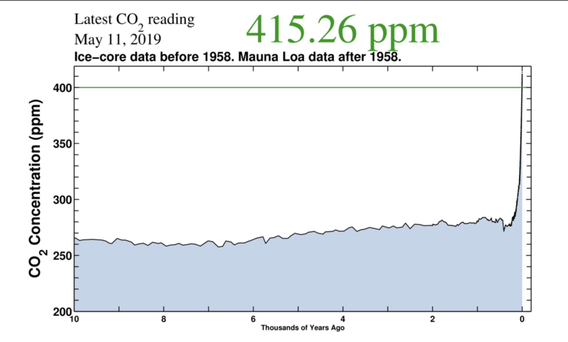
If pre-industrial there wasn’t an equilibrium we would have seen a spectacular rise which we did not see. QED
Hans Erren,
Ice core data lack temporal resolution to show rises similar to those measured at Mauna Loa. Also, early publications of ice core data show pre-industrial values of atmospheric CO2 concentration that were over 400 ppmv (i.e. similar to present day Mauna Loa atmospheric CO2 values) but all such values are now assumed to be “biological contamination” and are deleted from recent publications of the data sets.
Stomata data show pre-industrial atmospheric CO2 rises similar to those measured at Mauna Loa since 1958. Ice core data cannot show such rises.
If pre-industrial there was an equilibrium we would have seen a spectacular rise indicated by the stomata data, which we do. QED
Richard
During the several glaciations there was a spectacular decline in CO2, probably primarily because CO2 is more soluble in cold water than in warm water. It is reasonable to expect that as the oceans warmed, there was “a spectacular rise,” which anthropogenic emissions contribute to. However, it is less than 4% of the total flux. That rise is continuing, although not necessarily at the same rate as the decline because the dissolved CO2 is sequestered in the ocean bottoms for about a thousand years before it can outgass.
“What you’re missing is, the assumption that everything was “in balance” before the “new guy” contributed candy, without any actual measurement of the amount going in and the amount going out, which was nothing more than guesswork based on “estimates.””
Estimates that are good enough when using the Grisp2 ice-core to justify a global temp correlation from a single location I might say.
The “amount going in” vs the “amount going out”, when in ~ balance will result in a quasi-stationary CO2 ppm.
Thus:
CO2 ppm barely changed by 20 ppm in the thousands of years prior to the Industrial revolution and land use changes before it.
And where has CO2 ppm gone since?
OH NOES! A HOCKEY SCHTICK!
Anthony Banton,
The two data sets you have spliced in your graph have different temporal resolution.
Assuming the ice core data show ancient atmospheric CO2 concentration (they don’t but I am trying to be kind to you) then the UN IPCC says they have temporal resolution of 83 years.
The Mauna Loa data have resolution of individual months or years.
So, to compare the two data sets you need to average your Mauna Loa data with an 83 year running mean, but that is not possible because the Mauna Loa time series started in 1958 so is twenty years too short for you to obtain a single smoothed comparable datum!
You have compared ‘apples to sticks of Blackpool rock’ then said, “See, there is a coconut”. Who taught you this trick, Michael Mann?”
Richard
“So, to compare the two data sets you need to average your Mauna Loa data with an 83 year running mean”
Garbage.
Mike Edwards,
The “garbage” is yours.
Glacial ice is formed from precipitation (i.e. snow). The settled snow is porous and is called fern. The firn takes time to solidify and to seal (for explanation see e.g. https://www.britannica.com/science/firn ).
The IPCC says the Grisp-2 glacial firn takes 83 years to seal.
Air is pumped in and out of the porous firn by variations in air pressure (i.e. weather), and this mixes the air in the firn until the firn seals to become solid ice., Hence, any sample of air trapped in the solid ice is a mixture of air compositions from the 83 years when that ice was firn.
Your comment adds nothing to the thread except to cast doubt on any other contribution you choose to make.
Richard
How come you start your graph at the end of the last glaciation? And, why are you splicing high resolution data to low resolution data? David Middleton has remarked about this several times!
Please see my response to DrEd.
Nope. All you’re doing here is emphasizing uncertainty. The claim that there is an assumption of prior state being in equilibrium is just another strawman argument.
It doesn’t matter if the office was at steady state prior to the new hire coming on board. There could have been a trend either way—accumulation, depletion, or steady state.
It doesn’t change the fact that if someone contributes without consuming, that increases an accumulation trend or reduces a depletion trend.
I think that the major flaw in your analogy is the assumption that the sinks continue to absorb at the same rate even in the presence of an increase in the partial pressure of CO2 in the atmosphere.
Analogies are useful, but they also have limitations in that they are rarely exactly like the real world, which is why they are useful!
See my reply to DrEd.
I did see your reply to DrEd. I don’t think that it is responsive to my comment. I basically gave a reason why the office staff would increase their take of candy.
Yes, yes, the office staff may increase its candy intake, and the biosphere may increase its carbon-dioxide intake. But if that’s all you’ve got, I don’t think you’ve demonstrated what you think you have.
Again, maybe I’ve misunderstood you. But my impression is that you seem to think your candy analogy establishes that carbon-dioxide concentration would still be about what it is today even if our last 300 years’ emissions had been no greater than they were over the 300 years before that. If so, your logic is as bad as I had feared, for the reason given above by Rich Davis.
You did misunderstand me. The primary point of the candy analogy was to show that it is highly improbable that the annual increase in CO2 is the CO2 emitted by humans. Therefore, the other sources must also be increasing, and/or the sinks are decreasing. The latter is probable because CO2 is less soluble in warm water than cold water.
Despite my attempts to get clarification I still can’t tell for sure whether what you think you’ve established is merely the relatively non-controversial proposition that human emissions aren’t the only cause of the carbon-dioxide-concentration change we’ve observed over the past century even though most of the change wouldn’t have occurred in the absence of human emissions.
But I’m not going to beat a dead horse.
oh good lord … to talk about measuring “global” CO2 … when 1) we can’t measure it globally 2) its not even close to a well mixed gas is simply nonsense on stilts …
just curious- and just wondering, is it well understood- the degree to which that gas is well mixed, globally? Quantified?
The real problem is that there is no official, accepted definition of “well mixed” with respect to CO2. It obviously isn’t as well mixed as nitrogen, but is not as heterogeneous as water vapor.
How heterogeneous is water vapor? How do you know that?
Simple observation. One can observe rain falling in one area while standing in an area that is dry. Sometimes the rain never makes it to the ground, evaporating on the way down.
Mr. Zorzin:
I hope you find the below helpful.
Your WUWT ally for science truth,
Janice
P.S. I admire your persevering enthusiasm for truth (from reading many of your comments) 🙂 .
___________________________
“1.1.1 Descriptions of atmospheric behavior The mobility of a fluid system makes its description complex. Atmospheric motion redistributes mass and constituents into a variety of complex configurations. Like any fluid system, the atmosphere is governed by the laws of continuum mechanics. They can be derived from the laws of mechanics and thermodynamics … .”
(Source: Physics of the Atmosphere and Climate, 2d Ed. (2012), Murry L. Salby, Excerpt, Cambridge University Press 978-0-521-76718-7, p. 1
https://assets.cambridge.org/97805217/67187/excerpt/9780521767187_excerpt.pdf )
“Of the factors influencing atmospheric behavior, gravity is the single most important.”
(Ibid. at 2)
“The Earth’s rotation, like gravity, exerts an important influence on atmospheric motion and, hence, on distributions of atmospheric properties. … rotation tends to stratify properties meridionally, just as gravity tends to stratify them vertically. ***
… interwoven in a complex fabric of radiation, chemistry, and dynamics that govern the Earth-atmosphere system”
(Id. at 3)
“Below 100 km, the mean free path is short enough for turbulent eddies in the circulation to be only weakly damped by molecular diffusion. At those altitudes, bulk transport by turbulent air motion dominates diffusive transport of atmospheric constituents. Turbulence stirs different gases with equal efficiency. Mixing ratios of passive constituents are therefore homogeneous in this region. Those constituents are said to be “well mixed. …”
(Id. at 9, 10)
“Table 1.1. Atmospheric Composition. Constituents are listed with volume mixing ratios representative of the Troposphere or Stratosphere, how the latter are distributed vertically, and controlling processes Tropospheric Vertical Distribution
Constituent *********Mixing Ratio (Mixing Ratio)********* Controlling Processes
N2 .7808 ****************Homogeneous ***********************Vertical Mixing
O2 .2095 ****************Homogeneous ***********************Vertical Mixing
…
∗CO2 380 ppmv ********Homogeneous **********************Vertical Mixing
…
∗ Radiatively active
(Id. at 4)
***********************
Edit was mainly to insert all the ******* (the only way I could put spaces into the copied table — the “space” char doesn’t “stick” for me 😐)
https://www.bing.com/videos/search?q=Oco+2+Satellite&&view=detail&mid=54F2D3BEC8AEEC0EB1F354F2D3BEC8AEEC0EB1F3&&FORM=VDRVRV
You ain’t gonna know what you got till its gone..
Can’t recall where I found this so here it is on my Dropbox
https://www.dropbox.com/s/2fcj8k4m7pqq5lj/USA%20Swichgrass%20CO2%20Flux%20-%20Copy.PDF?dl=0
The pic is a screenshot off the first page:
See where it says:
“Knowledge of the factors controlling…blah blah”
In no special order those are:
## The ‘Biomass’ you see, the trees. plants and ‘Fuel Load’ are not the major source of of the CO2 – its coming from the soil and the dirt – controlled by bacteria and hence the noted ‘Temperature dependence’
Look downwards instead of up at the Dancing Angels – you might find something to keep you warm down there.
The Angels nor Phlogiston are not gonna help you survive desert life
I see you got a down vote so I helped by canceling it. If you believe that molecules emit at certain frequencies then you must also ask where does the 15 um radiation from the surface of the globe arise. It only makes sense that as the sun warms the soil, that CO2 in the soil begins to emit at 15 um. Otherwise all the other molecules of various substances would have to add together to arrive at the power that is supposedly emitted by the earth at 15 um.
Those singular troll down votes are as insidious as spray-painted graffiti. You paint over it and there is more the next day.
Gas molecules absorb/emit at certain frequencies, however solids and liquids will emit as black bodies. So the 15micron radiation from the surface is not due to CO2 but due to all the surface molecules. In the atmosphere though the absorption is predominantly by H2O, CO2 and O3 at their respective wavelengths.
Shame on NASA for highly unscientific suppression of Global CO2 maps. What else can we conclude but that this organization presents data that supports totalitarian science with fanfare, but buries meme threatening data or ‘reanalyzes’ (destroys) it and makes it impossible to download.
They did the same thing with the “Great Greening” of the planet. They presented their finding in 2014(?), but the Dark Side obviously wasn’t happy about this because it drew attention to the overwhelming benefits of added CO2- both for wildlife habitat and a remarkable doubling and redoubling of global harvests.
The Dark Side tried to sell the proposition that this was bad news indeed and then fell silent. NASA. Recently, their scientists published a worrying article on greening in the high Arctic, meanwhile ignoring the the real elephant, the expanding forests and shrubs fringing and penetrating hot arid regions of the globe and India becoming a supplier of grain exports.
These innovative satellite projects belong to the taxpayer! Importantly, they provide valuable data that is being obscured, refiddled and made difficult to access because it tells us that their Lysenko science is wrong.
Unfortunately nothing belongs to the taxpayer any longer. They belong to quasi-judicial agencies and bloated bureaucracies. The taxpayer, like an indentured servant, exists only to carry the load.
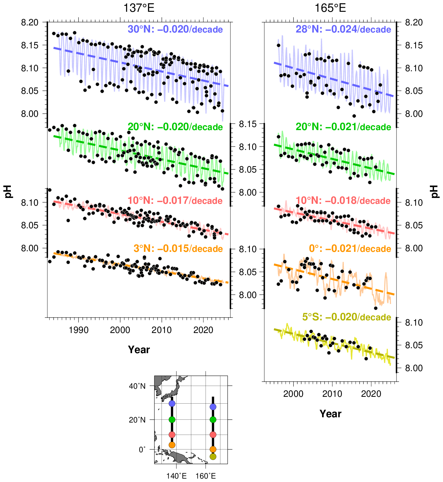
“An alternative interpretation for the current paradigm is that, against a background of relatively constant anthropogenic emissions, the warming Earth forces an increase in ocean out-gassing and biogenic emissions during the seasonal CO2 ramp-up phase.”
Seasonal CO2 follows the annual insolation temperature cycle response like clockwork.
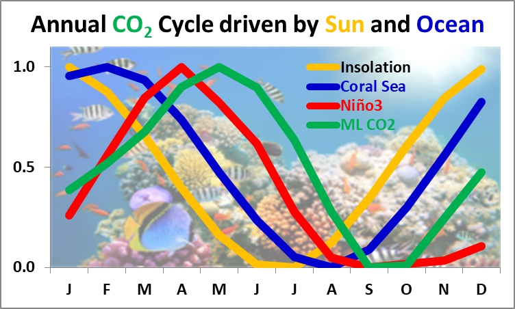
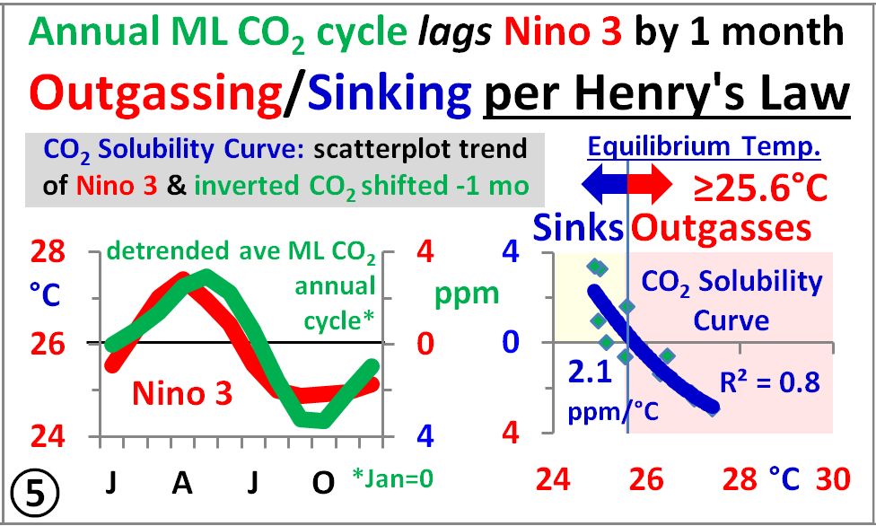
The important subject of what caused the upwards CO2 trend is answered by Henry’s Law, as temperature partitions the ocean into sinks and sources that have changed in relative sizes and temperatures since the early 1900s. The CO2 trend was driven by the growth in SST≥25.6°C, which increased nearly 50% in the last century as the modern maximum in solar activity warmed the ocean.
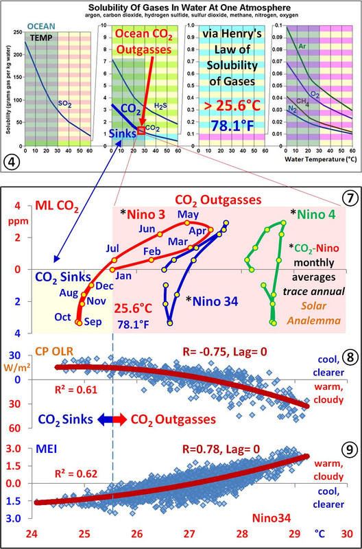
Panel 7 of the last image shows monthly CO2 vs Niño3, Niño34, and Niño4, which all trace out a solar analemma relative to location, further verifying the annual insolation control over atmospheric CO2.
This means the ocean sources/sinks allow more/less CO2 to remain in the atmosphere regardless of source, as Clyde Spencer generally said.
That may be a spurious correlation because the drawdown is a function of both temperature (above freezing) and duration and intensity of sunlight for photosynthesis. It appears that the ramp-up is a result of bacterial decomposition and tree respiration, which is less sensitive to land temperatures. Oceanic outgassing is temperature driven.
“That may be a spurious correlation …. Oceanic outgassing is temperature driven.”
Make up your mind. Why did you originally make the statement I responded to?
I provided direct evidence to support your point on outgassing and now I’m told outgassing is spurious? Which is it please? You’re not unknowingly engaging in some kind of doublespeak are you?
As far as I can see no one else but me has provided any detail here at WUWT as to how Henry’s Law operates in the ocean, which I started to do in 2019 after determining the outgassing threshold temperature.
Your otherwise nice article is speculative without this knowledge.
The point Greg Goodman made about imposing a sinusoid, in this case annual insolation, is shown to work perfectly in the composite I made just for you below, which has same one month lag as monthly Nino3 and ML CO2.
Mauna Loa CO2 is directly driven by southern insolation and integrated insolation warming, perfectly correlated with a one-month lag, accordingly, outgassing/sinking therefore greatly dominates the annual NH CO2 vegetative drawdown.
The point is, there are several things that directly impact the emission and absorption of CO2. Some of them, like bacterial decomposition, seem relatively insensitive to temperature, while outgassing is driven exclusively by temperature. Also, land responds differently than the oceans.
I’m afraid I’m missing something here. It looks to me like you are demonstrating a 3-month lag.
Clyde, the SH ocean warming starts when the thick gold line representing SH seasonal insolation starts increasing in September, and continues until the season changes at the top of the integrated SH insolation curve in early April, the red dotted line. Follow the blue arrow.
Peak CO2 in May follows April by one month, hence the one month lag.
SH summer insolation keeps the ocean warm enough for one more month of outgassing in May, until the season changes after the sub-solar point crosses the equator going northward, and then the southern ocean starts cooling from May to September, when the cycle starts over.
Dear Clyde
You will find a complete set of 30 images here. I communicated with OCO2 scientists leading up to the 15th April 2016 release.
I had the commentary figured out before I received the images.
I need to update the commentary as I have increased my knowledge a bit more since I posted this in June 2016. But you will get the idea. I should have looked at the 80 and 90km altitude movement timing rather than the 100km.
The 30 images are time sequenced against Mauna Loa for reference.
Just here to help, as I knew they would disappear.
https://blozonehole.com/blozone-hole-theory/blozone-hole-theory/carbon-cycle-using-nasa-oco-2-satellite-images
These images look familiar. Interestingly, your Fig. 2, which corresponds in time with my Fig. 1a, looks very different. Your pictures do not look like the COP-26 animation that Tillman linked to. How do we know what maps to trust?
I disagree with your interpretation of the CO2 actually migrating, but thank you for providing the imagery.
Clyde.
I have not seen the ones that Tillman referred to.
These are the first original images that were released. They were on a youtube video so I cut them from there before they removed the video. I also have the larger higher resolution ones that I downloaded from the OCO2 website a short time later. Take a copy of the ones from my site. If you want the larger higher resolution ones send me your email.
The NASA OCO2 folks later replaced them when they extended the time coverage and altered the density calibration eliminating the contrast and great detail that these provide. They are the real deal. The ones you provide are of little value for your post.
Clyde disagrees.
And yet the CO2 recorded at the Antarctica sites is always remains the same few ppm behind the NH sites. The only reason the Antarctica values are consistently slightly lower is the dilution factor when mixing into the SH lower emission atmosphere. Over 90% of all emissions are NH sourced.
Also how do those nasty chemicals that are produced and released in the NH that are consistently replenished annually and measured above Antarctica get there. The ones that theoretically destroy ozone,
Then, please explain why in my images the CO2 levels in the SH suddenly increase over a few weeks, when there are very few emissions down here. Look at my image #30 with the higher concentration of CO2 and then the dilution of Ozone in the same atmospheric tract in the following image.
They are inert and relatively insoluble, so they get transported presumably by the Brewer-Dobson circulation cells. CO2 dissolves readily in rain and sea water, and is taken out of the air by photosynthesis.
https://en.wikipedia.org/wiki/Brewer%E2%80%93Dobson_circulation
Three new peer-reviewed studies show that mankind’s emissions are irrelevant.
https://scc.klimarealistene.com/produkt/the-impact-of-human-co2-on-atmospheric-co2/
https://scc.klimarealistene.com/2021/10/new-papers-on-control-of-atmospheric-co2/
These detailed analyses also show a key feature of the observed increase of atmospheric carbon dioxide, one that was found earlier by Humlum (2013): Increased carbon dioxide comes from the tropics, not from temperate latitudes where mankind’s emissions are concentrated.
The truth is that there is no net accumulation of CO2 (either natural or anthropogenic) in the atmosphere beyond a year. The big sink in the Arctic is cold open water with some assistance of trees and grass. The annual ramp up is directly associated with the freezing of the Arctic ocean. The rapid decline is directly associated with the thawing of that ice. Within a year all the CO2 being delivered to the Arctic is absorbed by cold open waters and is readily consumed by phytoplankton blooms.
The biggest sink is cold water in clouds which returns CO2 to the surface in rain. Most of all CO2 emissions (both natural and anthropogenic) are returned to the surface by rain. The observed year-to-year increase in concentration is the result of year-to-year increases in natural emission rates. The more negative values of the isotope index reflect a greening of the oceans with a year-to-year increase in the decay of phytoplankton.
What then is your explanation for the Keeling curve?
Do a multi-linear regression of the MLO data on Artic sea ice concentration with a long-term function of 2*@pi*time(year). I have used cos(x/200)+sin(x/200) for the long-term function. Numbers greater than 200 make little difference in the resulting degree of fit which has an R^2 of better than 0.995, Thus, only four calculated coefficients produce an extremely good fit. The long-term function shows the year-to-year increase in natural emission rates.
What are the functions that you are using as independent variables in your multi-linear regression?
Fred
The image below may allow you to think that there is a direct relationship, but it is not correct. Both are controlled by the same atmospheric dynamics. There are bigger forces at play.
The image below is from Greg – climategrog
No accumulation beyond a year? How do you go from 280ppm to 420ppm without accumulation?
I think you’re confusing accumulation with residence time. Except for isotopic variety, all CO2 molecules are interchangeable. It doesn’t matter how long a particular molecule remains in the atmosphere, it matters how many CO2 molecules are in the atmosphere at any given time.
If I’ve said this a hundred times, I’ll say it a hundred more. When our annual “contribution” is 3-4%, then the “null hypothesis” should be that we are responsible for 3-4% of any increase in atmospheric levels, absent detailed measurements of all of the “sources” and “sinks” which tell a different story, which simply do not exist.
Assumptions of things being “in balance” based on what is essentially, scientifically speaking, crap for “data” is not a “fact,” is not “reality,” is not “truth” and is not even “data.” And it certainly isn’t “science.” It is just an assumption.
And policy should not be based on poorly supported assumptions, of which the notion that human emissions account for changes to atmospheric CO2 levels is just one of many, ALL of which have no solid empirical basis.
“The major sources of CO2 are not spatially associated with high population densities or industrial activity during the seasonal ramp-up phase, with the possible exception of China.”
As is to be expected as, as you say, ~ 96% comes from natural sources and China is the world’s major anthropogenic emitter.
“….. the warming Earth forces an increase in ocean out-gassing and biogenic emissions during the seasonal CO2 ramp-up phase. During the drawdown phase, the warming high-latitude waters are less effective at capturing the CO2 in the atmosphere. ”
Then how do you explain the reduction in oceanic ph?


For there to be a decreasing ph then the oceans must be a net sink of atmospheric CO2.
https://www.ipsl.fr/en/article/socat-version-2021-for-quantification-of-ocean-co2-uptake/
“Figure 1. Left: Map of the new sea surface CO2 fugacity (fCO2, µatm) added in the SOCAT version 2021 (mainly for the period 2018-2020). In the Atlantic and Southern Ocean one identified the sailing route of the Vendée Globe race (Sea-Explorer, skipper Boris Herrmann). Right: All data in SOCAT for the period 1957-2020. Squares identified CO2 probes on moorings. The atmospheric CO2 level in the atmosphere being around 410 ppm today, the blue-green region (resp. yellow-orange-red) identified ocean CO2 sink (resp. source). Note few observations available in recent years in the south Pacific and Indian Oceans that calls to use data-based approaches to extrapolate the fCO2 field and calculate integrated air-sea CO2 fluxes at large scale (Figure 2) or to estimate change in pH (ocean acidification) in the oceans (Figure 3). D. R.”
Also, given that burning fossil fuels uses atmospheric O2, then you need to explain this also …..
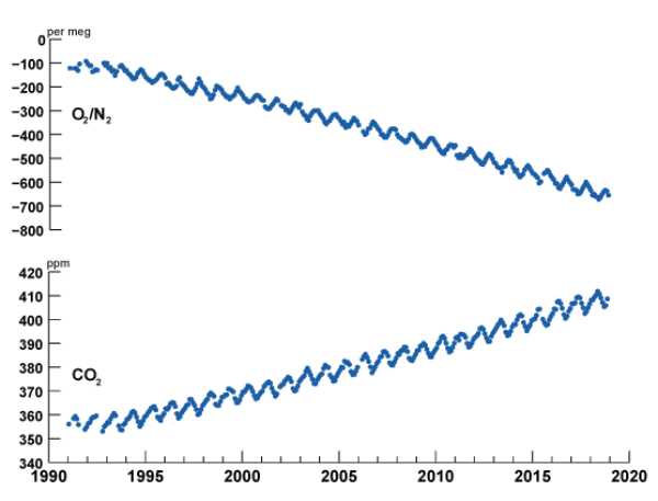
https://library.ucsd.edu/dc/collection/bb9492732t
HOTS = Station Aloha


Context… What a concept!
Thank you for the contextual graphs, David. 🙂
I could have broken out Sverdrup, Johnson & Fleming… 🍻
There is no question that the CO2 is increasing in both the atmosphere and oceans. The question is whether it can be attributed to anthropogenic sources exclusively or even principally.
Your data shows a clear seasonality, which suggests a correlation between pH and temperature and/or sunlight. Runoff from agricultural land is fertilizing the oceans, providing a stimulus to phytoplankton, as is increasing temperatures. As calcifiers proliferate, they extract (bi)carbonate, which will drive down pH. As phytoplankton blooms die off, they will consume oxygen in the water.
I don’t think that a qualitative analysis will answer the issues you raise to anyone’s satisfaction. Someone is going to have to address the quantitative analysis.
As I understand it, the OCO-2 satellite has now been superseded by OCO-3 which is attached to the International Space Station.
There’s also a link to OCO-3 Data, Maps etc. at the below:
https://ocov3.jpl.nasa.gov
OCO-3 has a different focus. It is trying to define the industrial and urban emissions, to the exclusion of what is going in the Amazon and Congo, and the northern boreal forests.
Yep, while OCO-3 apparently has increased resolution, it can also be ‘aimed’.
They’ll create a mosaic of industrial emissions to show it’s all our fault.
When the only tool you have is a hammer . . .
In the 1970s, urban mapping came into vogue with the Clean air Act. The intent then was to identify those structures (apartment complexes, government buildings, et alia) whose heating systems were not being maintained or were of older technolgies, so that change could be directed in replacement with systems that provided heat without burning fuels with high sulfur content thus polluting the urban atmosphere and causing breathing issues with the local population.
I suspect, as you indicate, OCO-3 will used for other purposes.
Already being done!
2017 OCO-2 data analyses and paper releases in SciMag destroyed the Bern Model and NASA super computer simulation of it produced in 2014. This was an “the emperor really is naked” moment in the whole Emperor’s New Clothes bamboozling of the public on CO2 growth.
Without CO2 growth being causally linked to global temperature increases of the last 70 years, the climate scam unravels rather calamitously.
So something had to be done when those SciMag papers destroyed many of the assumptions in the climate scriptures of the Bern model.
1)No more OCO-2 data papers.
2) make OCO2 data difficult for anyone but deep pocketed researchers on the government dime to process and interpret.
3)the climate clothiers had to move on to OCO-3, a much more footprint nadir focused and exclusionary instrument on the ISS rather than a broadly global view from a satellite in the A-train of our polar orbiting science sat array.
“Therefore, it becomes very unlikely that the same person brought all of the remaining pieces. That is, having a large number of pieces of candy left over, all from the same person is highly improbable. ”
What a strawman of an analogy. Nobody who understands the carbon cycle says that every additional CO2 molecule in the atmosphere came from a human source. The claim is that all, or most, of the increased CO2 level was caused by the additional CO emissions. It doesn’t matter which specific molecule goes back into a sink, what matters is how many are left over each year.
Suppose you have a stable bank balance, with your annual income equaling your annual expenditure. Then someone (no questions asked) starts putting in a sum each year equal to 4% of your income, and you increase your spending by 2%, what happens to your bank balance? Is all the increase because of the extra money going in? Is it a defense to argue that it’s impossible to tell which of the additional dollars in your balance came from which source?
Nobody who understands the carbon cycle
will do anything but scoff at your bank account strawman of an analogy.
Native Source of CO2 – ~150 (96%) gigatons/yr : Human CO2 – ~5 (4%) gtons/yr.. (Salby at 36:34) Native Sinks Approximately* Balance Native Sources (i.e., net CO2) (37:01).
*Approximately = even a small imbalance can overwhelm any human CO2 (Native = 2 orders of magnitude greater than human)
(Source Murry Salby, Hamburg, 2013 (times above from this video):
******************************************
A plausible bank analogy would compare a typical personal savings account of < $15,000 with the balance sheet of the bank as a whole. The billions of debits and credits to the bank’s account, roughly in balance, would obliterate any debits and credits to that personal savings account.
EDIT (to my 12/16/21, 11:11AM comment) “The billions [of $$ in] debits and credits… .” 🙄
I’m lost with your bank analogy. Is the billions of dollars of debits and credits meant to represent the natural sinks and sources, and your < $15,000 meant to represent the human emissions? If so you need an analogy where your one bank account represents 4% of all the banks debits, and then explain why adding this extra 4% isn’t going to affect the banks holdings.
Then all you have to do is explain how the fluctuations which will obliterate the affects of your savings account applies to the real world, where there is no evidence that the 4% is being obliterated by natural fluctuations. If that were the case it’s difficult to see how we could be seeing such a consistent raise in CO2 levels.
You: “I’m lost.”
Me: Yes.
To find your way, watch the 2015 Murry Salby video here:
You may want to start at 4:30.
See also, Murry Salby, here in 2018:
Also, because you obviously did not watch it yet, please see also the Murry Salby 2013 Hamburg lecture linked in my 12/16/21 comment to you just above, at 11:11AM, on this thread.
“You: “I’m lost.”
Me: Yes.”
I apologize for trying to be polite about your feeble analogy. What I should have said is it’s meaningless and you need to come up with a better one if you expect me to take it seriously.
And if you think I’m going to waste 3 hours of my life plowing through lectures, just to figure out what you were trying to say, you may need to lower your expectations.
So. You don’t want to know the facts. Someone seeking truth would want to listen to a world class expert on climate. So be it, O Pitiful One.
Or you could just point me to his written work, or summarize his arguments for yourself.
OK, I’ve got as far as 3:53, and he already seems to mistaken and or misleading. He claims CO2 emissions were increasing linearly from 1990 to 2002, and then linearly from 2002 to 2014, but increasing at twice the rate. Then he compares this with CO2 levels, but for some reason only starts in 1995. He says the rate of increase was linear between 1995 and 2002, and then continued at the same rate after 2002.
Firstly, starting at 1995 is obviously a cheat as you can seen in his graph the overall trend is not linear, and his green line is below the CO2 level prior to 1995.
Secondly, these figures don’t agree with my calculations. True the rate of increase after 2002 is just over 2ppm / year, but the rate of increase from 1995 to 2002 is 1.7ppm / year. According to Salby the two rates are identical. According to my figures the later rate has increased by about 17%.
If you compare like for like, the trend between 1990 and 2002 is only 1.6 ppm / year, so there was actually an increase of 25%.
He’s also misleading by showing a graph for emissions that starts at 6 GtC, thus exaggerating the amount of change post 2002. It isn’t the rate of change that matters, it’s the total emissions each year. Eyeballing his graph, the average annual emissions in the 1990s were about 6.5 GtC, and after that about 8.5 GtC. That’s very roughly about a 30% increase, which is not that different than the observed change in the rate of CO2 increase.
Playing around with the data a bit, just to see how much Salby’s graph held up, I compared cumulative emissions, with the annual average CO2 level. Data from 1959 to 2020.
A statistically significant correlation with an r^2 value of 0.9996.
Made a bad mistake with the previous graph, which meant I was double counting different countries and also I think the units are wrong.
Hopefully this graph is more correct, though it doesn’t really change the result. r^2 is 0.9991.
My god, I also have to agree with Bellman. Might as well have griff chime in for my ultimate mortification.
So if my bank is profitable, my checking account increases and if my bank is losing money, my checking account is going down?
For once Anthony is right. I admit, having to agree with him gives me pause. (He probably feels the same if he’s paid any attention to my previous blathering).
Look, I don’t say that it matters that CO2 is rising (other than that it’s beneficial for plants). What I do say is that it’s pretty clear that we’re causing the rise from 0.028% to 0.042%, and so what?
Trying to argue that because we can’t empirically measure each source and sink with precision therefore we can’t reasonably acknowledge that humans caused this slight change is not reasonable. It helps discredit the skeptical argument about “climate change”.
We should be arguing that this is all good. We’re turning India into an exporter of grain. The empirical evidence of what ECS is would imply only more benefit until we exhaust economically-extractible fossil fuels.
The real future crisis is that the next glaciation will come and we will have used up the fossil fuel.
So if anything is urgent, it’s getting safe, inexpensive, abundant energy from nuclear power in place while we still have the capital to do so. But truth to be told, urgent is a major exaggeration. My children’s children’s children might start to see urgency if nothing is done during my grandchildren’s lifetime.
Further — in agreeing with Bellman/Anthony(??), you are arguing against two of the greatest current experts in climate: 1) Richard Lindzen and 2) Murry Salby. It will take a LOT evidence to refute those two… .
FYI: you mischaracterized my analogy (which was ONLY a quick counter to B.man’s nonsense and not AT ALL an attempt to analogize the CO2 budget/source/sink to any fine degree of accuracy).
Janice,
Did I miss something where you cited Lindzen on the topic of the impact of human emissions on atmospheric CO2? I’d be interested in reading/watching that.
“Anthony is the Bellman”
Libel.
Specious claim.
For clarity—Anthony Banton, not our gracious host. Of course I always agree with that Anthony!
That’s what I assumed. It’s still libelous. (Not sure which of us would find it most libelous!)
Since you’re making appeal to authority claims rather than discussing the actual hypothesis, I doubt that any further words from me will persuade you, Janice. I don’t see how to improve on this old WUWT posting by Rud Istvan:
https://wattsupwiththat.com/2017/05/13/is-murry-salby-right/
Rud referred to an earlier post by Willis Eschenbach that is also very well worth reading:
https://wattsupwiththat.com/2015/04/19/the-secret-life-of-half-life/
Clyde Spencer,
Thank you for your fine article which is timely because Ed Berry has today announced publication of his paper in the formal literature.
As you say, there is much evidence that human emissions of CO2 do not directly effect the rise in atmospheric CO2 concentration as observed first at Mauna Loa (since 1958) and now also measured at several other places.
Importantly, changes to atmospheric CO2 concentration follow changes to global temperature at all time scales.
At long term the ice core data indicate CO2 increases after warming at centennial and millennial time scales
Present day circumstances are indicated by direct measurements which indicate changes at the shortest term. The seminal work on this was
Kuo C, Lindberg C & Thompson DJ, “Coherence established between atmospheric carbon dioxide and global temperature” Nature 343, pages 709–714 (1990)
Its Abstract says,
(emphasis added: RSC)
That study was conducted using Mauna Loa data. Subsequent studies confirm its findings but show the lag of atmospheric CO2 concentration changes behind global temperature varies with latitude and is in the range 5 to 9 months.
Total anthropogenic CO2 emissions (i.e. CO2 emitted by human activities) are less than the cumulative errors in the measurements of CO2 emissions from nature. This suggests that nothing can be shown about causality of atmospheric CO2 concentration with any certainty, and that is what I concluded in my studies of the subject. However, Ed Berry has developed from some of my thoughts to obtain a breakthrough in understanding which I and all other authors failed to make, and this has enabled him to devise a method to quantify the natural and anthropogenic contributions to the rise in atmospheric CO2 concentration.
Ed Berry posts a paper of mine on his blog and has colour (blue) coded my thoughts from which he developed his own ideas. This can be seen at
https://edberry.com/blog/climate/climate-co2/limits-to-carbon-dioxide-concentation/
and Berry has has also posted on his blog a preprint of his paper that reports his quantification of the natural and anthropogenic contributions to the rise in atmospheric CO2 concentration. This can be seen at
https://edberry.com/blog/climate/climate-co2/preprint3/
His formal paper is available from behind a paywall at
The impact of human CO2 on atmospheric CO2 – SCC (klimarealistene.com)
By way of explanation, I add two facts about the carbon cycle for consideration.
(a)
The carbon cycle affects atmospheric CO2 concentration and is affected by the equilibrium state of the climate system. For several reasons (e.g. the earth’s orbit and axial tilt), the climate system is always ‘seeking’ equilibrium and never attains it. Also, the climate system is observed to be bi-stable ( i.e. it is stable in glacial and in interglacial states) and its equilibrium condition must differ for each stable state.
(b)
The carbon cycle is part of the global climate system which is more complex than the human brain (e.g. the carbon cycle has more interacting components, e.g. biological organisms, than the human brain has interacting components, e.g. neurones). Nobody claims they can construct a predictive model of the human brain but some people claim they can construct a predictive model of the global climate by assuming one parameter (atmospheric CO2 concentration) controls all global climate behaviour(s).
Again, thanks for your fine article above.
Richard
Thank you Richard for your excellent comments regarding Ed Berry’s recent paper.
I was going to post here until I saw your note.
Best wishes for the Holidays, my friend.
Post Script
In other news, it’s going to be a cold Christmas in Europe:
We can expect further extreme cold in January and February 2022, based on the cold Nino34 area and the vagaries of the Polar Vortex.
EUROPE FORECAST A BITTERLY COLD AND SNOWY CHRISTMAS, VIRUS LEAK, + WASHINGTON POST (& GOOGLE) ATTACKS ELECTROVERSE…?
December 16, 2021 Cap Allon
The truth always prevails… eventually.
And yet, we see the seasonal ramp-up peak in the northern hemisphere in May, which is about the time that the trees begin to leaf out. That suggests to me that the lag is probably no greater than a couple of weeks for terrestrial photosynthesis to start drawing down the CO2. It may be longer for the oceans. Also, the decline in photosynthesis might be slower as a result of different species reacting differently to declining sunlight and temperature.
I also have a friend who is a pretty good statistical analyst and this is what he found using time series analysis. His independent variable was ENSO 3-4, but it indeed showed the similar amount of lag for the rise in both temperature and CO2.
Jim Gorman,
Thanks for that info.
Do you have a formal reference to your friend’s work, please?
My request is solely because I would like to cite the work.
Richard
To whomever it concerns,
Again an unexplained negative vote has been given to a post I made. In what way is a negative vote warranted by a request for additional information together with a statement of the reason for the request?
Richard
The following plot is just a simple visualization of the direct relationship between a major El Niño (2015-2016) based on reported Oceanic Niño Index (ONI) values (3-month rolling average of Niño 3.4 region sea surface temperature) and the CO2 trend at Mauna Loa, as published by NOAA in November 2018.
NOAA: “The red lines and symbols represent the monthly mean values, centered on the middle of each month. The black lines and symbols represent the same, after correction for the average seasonal cycle.”
I added the approximate longer term trend in CO2 growth rate (dashed blue line) before and after the obvious increase (about double the pre- and post-rate of growth of CO2) and added a schematic representation of the ONI data.
The dates can be derived from the monthly data points on the black line: the first value is for January 2014. The start of El Niño is in November 2014 and peaks in November/December 2015. Hope this is of some interest.
The fact is that natural emission rates increase from year-to-year much more than anthropogenic emission rates increase from year-to-year. Using your bank account, this is like getting a cost of living raise each year amounting to 4%.
Do you have any evidence for that claim?
My main objection to all these claims of natural emissions being the cause of the increase, is that it’s a huge coincidence if these natural changes coincided so well with the known increase in human emissions, causing a very smooth increase which perfectly matches the rate of human emissions.
Human emissions are a function of the global population. The global population increase is assisted by increasing temperatures and a CO2-enriched atmosphere, which helps increase agricultural production. Not such a “huge coincidence!”
So now you just have to show how and why CO2 increased at such a steady rate over the last 60 years, and how it caused the population to increase at just the right amount, that their emissions just happened to be such a perfect fit for the increasing CO2. And why that’s easier to accept than the human emissions being the cause of the increased CO2.
Then you could try to explain where all the human released CO2 went.
See this graph from:
https://wattsupwiththat.com/2016/02/26/analysis-of-the-relationship-between-land-air-temperatures-and-atmospheric-carbon-dioxide-concentrations/
If you are going to put the equation in the graph it would help if you use a different scaling, so that you can see the coefficients. As it stands your equation is just saying y = 296.232.
Apart from that I’m not sure what you think this correlation demonstrates. You say that anthropogenic emissions are a function of population size, then claim that population size strongly correlates with CO2 levels. An obvious corollary would be that there is a correlation between anthropogenic emissions and CO2 levels.
At best you could be arguing that either rising CO2 levels are caused by emissions, or directly by population size.
But you want to argue the converse, that population size is caused by CO2 levels, with something else causing the rise in CO2. The trouble is from the statistics any of these is possible because we have three smoothly rising data sets, so any correlation will be near perfect. The question is which is more plausible.
1) Humans put additional CO2 into the atmosphere, which leads to a rise in atmospheric CO2.
2) CO2 starts rising for other reasons, which leads to a rise in population and us burning fossil fuels, which leads to an increase in CO2 emissions, which has almost no effect on the rising CO2 levels.
You remarked, “So now you just have to show how and why CO2 increased at such a steady rate over the last 60 years, and how it caused the population to increase at just the right amount, that their emissions just happened to be such a perfect fit for the increasing CO2.”
Well, first off anthropogenic emissions is not “such a perfect fit.” The annual increase is about 40% of the anthro’ emissions.
The graph addresses your remark. The assertion is that increasing temperatures and CO2 have allowed an increased production of food, increasing the fecundity of humans. More humans use more fossil fuels. They are all interconnected. It is not a simplistic case of y=mx+b.
https://scitechdaily.com/new-research-shows-plants-are-photosynthesizing-more-in-response-to-more-co2-in-the-atmosphere/
Cumulative emissions are a very good fit to the increase CO2, see the graph I posted elsewhere. It doesn’t prove anything, anymore than your graph proves that population increase is causing the CO2 rise, or the CO2 rise is increasing the population.
But the logic that putting extra CO2 into the atmosphere will increase the amount of CO2 in the atmosphere is stronger than the argument that CO2 rose for some unspecified reason and that caused more people to appear.
The fact that as you admit we are putting more CO2 into the atmosphere than the amount needed to increase it, is the point. You do not need any additional source of CO2 to explain the rise, our emissions more than explain it. It’s absurd to assume that nearly all the CO2 we put into the atmosphere goes into sinks and then try to find another explanation for why the CO2 is increasing.
It is partitioned into all the sinks in proportion to the size of the reservoirs.
You again seem to be obsessed with the actual carbon atoms rather than the number. If I put x amount of carbon atoms into the atmosphere, maybe for some weird reason they all end up in sinks, but everyone of my atoms that ends up in a sink prevents a natural atom from going there. Hence the number of carbon atoms in the atmosphere goes up regardless of which particular atoms remain.
Your proposition assumes a linear response across the board from seasonal flora to seasonal temperatures across the ocean to ENSO cycle variation. IOW, well mixed turbulent flow. None of what you claim has any basis in actual analysis of data.
Nothing in this climate is linear, it is all based on cycles with varying phases amongst the various phenomena including CO2 absorption by the oceans and land. CS has tried to analyze some of this using actual data. You have not. Annual averages hides so much activity from the sun and orbital changes that one can not simply look at annual averages and surmise what changes are happening due to anything throughout the year.
The only assumption I make is that carbon atoms do not vanish.
To paraphrase Bill Clinton, it all depends on what the meaning of “vanish” is.
CO2 can hide in trees for decades. It can hide in the deep ocean for almost 1,000 years. It can hide in permafrost for thousands of years. It can hide in rocks for hundreds of millions of years, both as coal and limestone. If subducted into the mantle, it may hide for billions of years. When hiding, or sequestered, it has the properties of something that actually did vanish — it is difficult to impossible to measure.
Somehow I don’t think the CO2 we’ve released has already turned back into coal. And if it has, why has it only happened to the anthropogenic CO2?
However, this might be an answer to the question “why, despite putting lots of CO2 into the atmosphere, has atmospheric CO2 not increased?”. But the question I’m interested in is why, given the CO2 did increase in line with what we’ve put in, do some think it’s plausible that all the CO2 we’ve added immediately vanished, but at the same time some other process increased the CO2? How did the vanishing processes distinguish between anthropogenic and the other sort of CO2? And why, if the increase in CO2 is coming from existing sources, do we not see a reduction in the CO2 sinks?
No, it does not. Never he claimed this. A strawman again.
Spencer need not prove anything of the sort. Simple logic tells us that increased industrialization (with the inherent increase in human CO2 emissions) more likely than not increases human welfare and population.
The burden of proof is on YOU.
Time for YOU to come up with some data.
“Simple logic tells us that increased industrialization (with the inherent increase in human CO2 emissions) more likely than not increases human welfare and population.”
I’m not denying that at all. It’s Spencer who seems to be denying any relation between industrialization and population. He’s claiming that CO2 increased, and that’s what caused the population increase.
It is
turtlesfeedback loops all the way down.You were much too kind to his analogy.
A number of replies, all along the lines that changes to natural sinks and sources could cause some of the increases, but not referencing my main objection to this article, which is the strawman argument that it’s very unlikely that every M&M could belong to the same person – and hence by analogy that it’s very unlikely that every additional molecule of CO2 in the atmosphere came from an anthropogenic source. If that isn’t the point of the article, then the author needs a better analogy.
How do those two statements differ functionally? That is, how can the atmospheric CO2 concentration increase be caused entirely by additional CO2 emissions unless all the additional CO2 is anthropogenic?
I’m saying that less than 4% of the increase is anthropogenic and the rest of the increase comes from the other natural sources.
I have a jar with 300 green M&M’s in, every so often I pour in another 25 green ones, mix everything up and then pull out 25 at random. Over the cycle the jar is in equilibrium, always has 300 green M&M’s in. Now someone, for no good reason, throws in an extra red M&M in every time I put my 25 in. I still mix it up and pull out 25 at random. This may or may not include that red one.
Each cycle the number of M&M’s in the jar increases by 1, so after 100 cycles there are 400 M&M’s in the jar. What proportion will be red? I’m not sure, but it’s highly unlikely to be 100 as that would imply I’ve never pulled a red one out. If this went on long enough the proportion of red ones would approach 4%, but for most of the time the proportion is likely to be well below 4%.
So the question is, what proportion of that rise in M&M’s was caused by those additional red ones being added?
Also note, that for this example to be more correct, you have to imagin I have a big bag of M&M’s I use to add to the jar, but also where I put the ones I take out. The natural sources of CO2 are also mostly the sinks. CO2 goes into the oceans and plants, and comes out again some time later.
This means that as I start pulling out red M&M’s, I’m putting them into the big bag, and there’s then the possibility that I will be adding some red ones back, even though this appears to be a natural source.
What you again have missed is that as the number of M&Ms increases, the analogue, the partial pressure of CO2, causes an increase in what is absorbed by the sinks. That is, your extraction doesn’t stay constant at 25. Instead, it has to increase.
I was trying to keep it simple, in order to illustrate how it’s possible to have all the increase caused by adding additional M&Ms, but not have all the additional M&Ms coming from the new source.
But if you prefer, change the number each cycle to 50, have our interloper add 2 new red ones each cycle, whilst you take out 51 each cycle. How many red M&Ms do you expect to see in the jar, once the total has increased by 100?
In the mean time, the analogy now requires that your big bag of M&Ms is also getting fuller, entirely caused by these additional red M&Ms.
Your analogy is flawed. For your theory that anthropogenic CO2 is responsible for the entire accumulation of CO2 you must assume that red M&M’s are never withdrawn from the jar and that only green ones are removed so that the increase is only attributable to the red M&M’s.
There are a multitude of other permutations, but the end result is that there are more red ones added each year that green ones taken out.
As far as CO2 is concerned, I have seen no experiments that show quantitively where the various isotopes enter sinks at varying rates. Perhaps you could provide some references that deal with this. I would appreciate the educational benefits.
“…you must assume that red M&M’s are never withdrawn from the jar and that only green ones are removed so that the increase is only attributable to the red M&M’s.”
The whole point of the analogy is that you don’t have to assume that. You could remove every red one, have a jar full of nothing but green M&Ms, and it would still be the case that all the increase was caused by adding the red ones.
There are all sorts of problems with your analogy, and so your understanding of the carbon cycle.
CO2 in the atmosphere is rising approximately linearly, while mankind’s release of CO2 is going up exponentially. If there was some magic balance already in place then we should see atmospheric CO2 going up in concert with anthropogenic CO2 – instead they seem decoupled except for they are both going up.
You seem to be imaging that nature had some magic hard line boundary on how much CO2 it can consume, and somehow it balanced this. The fact is nature will simply adjust to any increase OR decrease in CO2 over a suitable amount of time, with a lower limit set by plant’s requirements for photosynthesis. Nature will gladly expand consumption of CO2 if it’s available – some going to biology and some to chemistry in sea water.
The belief in a magic optimal “PPM for atmospheric CO2” is not scientific. The belief that atmospheric CO2 concentrations do not vary is not scientific either. Ice cores are a poor proxy for measuring CO2 levels – one can only hope they represent an average over 100 year periods if CO2 chemistry is indeed completely halted within the ice over thousands of years.
“CO2 in the atmosphere is rising approximately linearly, while mankind’s release of CO2 is going up exponentially.”
I’m pretty sure neither of those things are true. I’ll check for you when I have more time.
“If there was some magic balance already in place…”
There’s nothing magic about a balance. Everything else being equal it follows from the fact that it’s the same carbon being passed around all the time.
If there wasn’t a balance then there would be nothing stopping CO2 from decreasing to nothing, or increasing indefinitely.
“Ice cores are a poor proxy for measuring CO2 levels – one can only hope they represent an average over 100 year periods if CO2 chemistry is indeed completely halted within the ice over thousands of years.”
In other words, you’ve no evidence that CO2 levels have varied, you just don;t think the evidence is strong that they haven’t. This means is quite possible that past warm periods were caused by increased CO2, or the mini ice age was caused by a reduction in CO2.
There is no balance in the climate. That would require equilibrium amongst all the different phenomena that make up this planet.
Orbital changes, cloud changes, seasons, and on and on, keep tipping the climate constantly. Each variable has its own cycle and is influenced by a multitude of others. If something was in balance, it would be easy peasy to observe what that balance was and monitor it.
The fact that there are multiple sinks and sources, each with their own varying contribution to the whole makes the term “balance” simply impossible.
Think of climate as an orchestra where each time the conductor (the sun) signals a change, the sound originating from all the pieces vary also. Time is an essential part of this and is too often ignored thru averaging varying phenomena with no analysis of how other variables are changing at the same point in time. Even when using proxies, which are the ultimate averaging of the phenomena that occurred during their creation people only look at one or maybe two variables and ignore all the processes that went into creating that sample.
You missed the part where I said “everything else being equal”. Big changes in the environment can cause a change in the equilibrium – ice ages for instance cause a big drop in CO2. And seasonal changes cause a seasonal change in CO2. Year on year temperature changes can cause small fluctuations. But measured over any reasonable time frame the CO2 level is quite stable.
Bellman,
You say to Jim Gorman,
“You missed the part where I said “everything else being equal”.”
No, he addressed that when he told you,
“There is no balance in the climate. That would require equilibrium amongst all the different phenomena that make up this planet.”
Your contributions to this thread are sophistry worthy of Nick Stokes: they seem to be spin with no substance. Some are ridiculous (e.g. Your reply to some facts was, “I’m pretty sure neither of those things are true. I’ll check for you when I have more time.” An appropriate – and ridiculing – response is to say I’m pretty sure you are an idiot. I’ll check for you when I have more time.)
Richard
” Some are ridiculous (e.g. Your reply to some facts was, “I’m pretty sure neither of those things are true. I’ll check for you when I have more time.” An appropriate – and ridiculing – response is to say I’m pretty sure you are an idiot. I’ll check for you when I have more time.)”
Thanks, for reminding me. The two “facts” I was responding to, were
“CO2 in the atmosphere is rising approximately linearly, while mankind’s release of CO2 is going up exponentially.”
Let’s check the first fact.
Here’s the annual average of CO2 from Mauna Loa, with a linear fit. This does not look linear to me.
And here’s the same data with a cubic trend. It’s an almost exact fit. R^2 = 0.9994.
On to the second “fact”. Here’s anthropogenic emissions over the same period, with a linear fit.
It’s not so easy to tell if this is exponential or linear as there are periods of more rapid increase, especially after 2002, but also a flattening in the last decade.
Here’s the log of emissions.
So, yes, I think both of Robert Of Texas’ points were wrong.
He went on to say
“If there was some magic balance already in place then we should see atmospheric CO2 going up in concert with anthropogenic CO2 – instead they seem decoupled except for they are both going up.”
As I’ve said before the real test is to compare cumulative emissions, rather than year to year. Here they are, fitted with another quadratic fit.
And here’s what it looks like when I lay the cumulative emissions over atmospheric CO2.
The point of the final graph isn’t to prove that emissions caused the rise in CO2, but that one of the main claims made throughout this thread, that somehow there’s no statistical link between emissions and CO2 levels, is plainly wrong.
But given the fact that it would seem logical to assume that adding additional CO2 into the atmosphere would rise the amount of CO2 in the atmosphere, combined with the obvious strong correlation shown in the above graph, means I’m still wondering why so many here feel that something over than human emissions are the main cause of rising CO2 levels.
Argh – that’s a quadratic fit, not a cubic. (Why do I only notice these things after the edit period has ended?)
I agree there is no objective support to the claim that rising CO2 in the atmosphere is entirely due to human activities. I also agree that at least part of the increase must be due to warming if warming is happening in the ocean since water that warms has reduced capacity to hold CO2. I don’t feel this analogy is entirely relevant however. The bowl of candy could have the same amount left at the end of the party (the annual increase in atmospheric CO2) regardless of whether the few candies left came from one person or another (from natural or anthropogenic sources).
The argument alarmists are making isn’t that the extra CO2 molecules that remain in the atmosphere each year are only those from human activity, it is that the increase is entirely the net result of human activity even though clearly the CO2 molecules added from human activity have the same chance as any other molecules of being removed into carbon sinks.
As far as I am concerned no matter how much of the increase is due to human activity, we should be glad for the increase since the only objective effects we can measure are positive.
The point I was trying to make is “that the increase is entirely the net result of human activity” is improbable.
Clyde Spencer: “The point I was trying to make is “that the increase is entirely the net result of human activity” is improbable.” CORRECT
Andy Pattullo: “As far as I am concerned no matter how much of the increase is due to human activity, we should be glad for the increase since the only objective effects we can measure are positive.” CORRECT
Richard S Courtney: https://wattsupwiththat.com/2021/12/16/co2-party-having-fun-with-probabilities/#comment-3411944 CORRECT
Ed Berry’s latest is certainly a very important paper. In any case, the catastrophic human-made global warming (CAGW) hypothesis was disproved long ago – it is a decades-old fraud.
It is proved that atmospheric CO2 changes lag atmospheric temperature changes in the modern data record, and also by longer times in the ice core record. “The future cannot cause the past“– end of the phony CAGW crisis.
The (simplified) sequence is Nino34 Area SST warms, seawater evaporates, Tropical atmospheric humidity increases, Tropical atmospheric temperature warms, Global atmospheric temperature warms, atmospheric CO2 increases.
Pro-CAGW arguments have adopted the thuggish propaganda tactics of Lenin and Goebbels – Don’t argue the science, just incessantly repeat the same falsehoods and shout down / intimidate the opposition.
The alleged CAGW crisis is a decades-old scam that was concocted by scoundrels for political and financial gain – wolves stampeding the sheep – it never had any scientific credibility.
To understand how life came into being you have to understand the first reaction:
HCO3- + heat/UV = > CO2 (g) + OH- (around zero latitude . the equator)
To understand what stops life:
CO2 + 2H2O + cold = > HCO3- + H3O+ (+ /- 90 latitude)
There is been little or no change in the Antarctic, so CO2 continued to dissolve as normal.
Unfortunately, in the north, there has been explosion of heat,
According to this report: Sea Surface Temperature (noaa.gov) it appears that the rate of the warming of the Arctic ocean at the highest latitude is now about 0.7K/decade…..
Hence the zig zag of CO2 noted in Hawai…
Can’t have been me, I haven’t been to Hawaii for years!
Here in Southern California, when we have high temperatures, they are “higher than normal”, but when we have low temperatures (such as now), they are “lower than average”. A not so subtle attempt to push the argument?
The MSM is not above trying to manipulate their readership!
They may not be above it, but they’re certainly behind it!