By Andy May
My previous post on sea-surface temperature (SST) differences between HadSST and ERSST generated a lively discussion. Some, this author included, asserted that the Hadley Centre HadSST record and NOAA’s ERSST (the Extended Reconstructed Sea Surface Temperature) record could be used as is, and did not need to be turned into anomalies from the mean. Anomalies are constructed by taking a mean value over a specified reference period, for a specific location, and then subtracting this mean from each measurement at that location. For the HadSST dataset, the reference period is 1961-1990. For the ERSST dataset, the reference period is 1971-2000.
Most SST measurements are made by moving ships, buoys, or Argo floats, the reference mean is done on a specific location from a variety of instruments and at a variety of depths. In the case of HadSST, the reference is computed for 5° by 5° latitude and longitude “grid cells.” The cells are 308,025 square kilometers (119,025 square miles) at the equator, a square that is 556 kilometers (345 miles) on a side. The distance between each degree of longitude gets smaller as we move closer to the poles, but at 40° latitude, north or south, 5° of longitude is still 425 kilometers or 265 miles. These “reference cells” are huge areas in the mid to lower latitudes, but they are small near the poles.
To make matters worse, the technology used in the reference periods, either 1961-1990 or 1971-2000, is far less accurate than the measurements made today. In fact, NOAA weights Argo float and drifting buoys, introduced in the early 2000s, by 6.8X, relative to the weight given to ship’s data (Huang, et al., 2017). The Hadley Centre says that Argo floats reduce their uncertainty by 30% (Kennedy, Rayner, Atkinson, & Killick, 2019). During the two reference periods almost all the data was from ships. This means that the greater inaccuracy of the measurements, relative to today, in the 30-year reference periods is significant. We might assume that the additional uncertainty is random, but that is unlikely to be the case.
On land, all measurements made in the reference period can be from the same weather station. That weather station may have stayed in precisely the same location the whole time. There are serious problems with many land-based weather-stations, as documented by Fall, Watts and colleagues (Fall, et al., 2011), but at least the weather stations are not constantly moving. Land-based stations are fixed, but their elevations are all different and since air temperature is a function of elevation, creating anomalies to detect changes and trends makes a lot of sense. Weather stations, on sea and land, are distributed unevenly, so gridding the values is necessary when coverage is insufficient. In some areas, such as the conterminous United States (CONUS), there are so many weather stations, that arguably, gridding is unnecessary and, if done, can even reduce the accuracy of the computed average temperature trend.
CONUS occupies 3.1 million square miles and has 11,969 weather stations in the GHCN (Global Historical Climatology Network). This is about 260 square miles per station. Each station provides roughly 365 observations per year, more in some cases, at least 4.4 million observations. This amounts to about 1.4 observations per square mile. The coverage is adequate, the stations are at fixed locations and reasonably accurate. The world ocean covers 139.4 million square miles. In 2018, HadSST had a total of 18,470,411 observations. This is about 0.13 observations per square mile, or 9% of the coverage in the conterminous U.S.
Any computation of an average temperature, or a temperature trend, should be done as close to the original measurements as possible. Only the corrections and data manipulations required should be done. More is not better. Sea-surface temperature measurements are already corrected to an ocean depth of 20 cm. Their reference depth does not change. The source and the quality of the measurements at any ocean location changes constantly. The computation of the reference period temperature is not made from one platform, not even one type of equipment or at one depth so the reference is very prone to error and severe inconsistencies. Who is to say the reference temperature, that is subtracted from the measurements, is as accurate as the measurement? It is generally acknowledged that buoy and Argo float data are more accurate than ship data and by 2018, the buoy and float data are more numerous, the reverse was true from 1961-1990 (Huang, et al., 2017).
On the face of it, we believe that turning accurate measurements into inaccurate anomalies is an unnecessary and confounding step that should be avoided. Next, we summarize how the anomalies are calculated.
HadSST anomalies
First the in-situ measurements are quality-checked, and the surviving measurements are divided into 1° x 1° latitude and longitude, 5-day bins. The five-day bin is called a pentad. There are always 73 pentads in a year, so leap years have one 6-day “pentad” (Kennedy, Rayner, Atkinson, & Killick, 2019). The pentads are grouped into pseudo-months and augmented by monthly values from cells partially covered in ice. Finally, each one-degree pentad is turned into an anomaly by subtracting its mean from 1961-1990 mean. The one-degree pentad anomalies are named “super-observations” (Rayner, et al., 2006). Finally, the one-degree pentads are combined with a weighted “winsorized mean” into a monthly five-degree grid that is the basic HadSST product. An attempt to correct all the measurements to a 20 cm depth is made prior to computing the monthly mean value for the five-degree grid cell.
Over the past twenty years, the average populated five-degree cell has had 761 observations, which is one observation every 156 square miles (404 sq. km.) at the equator. We subjectively consider this good coverage and consider the populated cells solid values. However, as we saw in our last post, not every five-degree cell in the world ocean has a grid value or observations. In round numbers, only 37% of the world ocean cells have monthly values in 2018, this is 8,186 monthly ocean cells of 22,084. Notice that the polar cells, which are most of the cells with no values are small in area, relative to the mid-latitude and lower latitude cells. Thus, the area covered by the populated cells is much larger than 8,186/22,084 or 37% of the ocean. I didn’t compute the area covered, but it is likely more than half of the world ocean.
ERSST anomalies
The basic units used in constructing the ERSST dataset are 2°x2° latitude and longitude monthly bins. A 1971 – 2000 average of quality-controlled measurements is computed for each bin. This average is subtracted from each measurement taken in the bin to create an anomaly. After this is done the various measurements (ship, buoy, and Argo) are adjusted to account for the global average difference in their values. The adjusted values are then averaged into 2°x2° monthly “super observations.” Buoy and Argo data are weighted by a factor of 6.8X the ship observations (Huang, et al., 2017). Since the year 2000, Argo and buoy data have dominated the ERSST dataset, both in quality and quantity. This is easily seen in Figure 1 of our last post, as the Argo dominated University of Hamburg and NOAA MIMOC multiyear temperature estimates fall on top of the ERSST line. This is also verified by Huang, et al. (Huang, et al., 2017).
The 2°x2° bins used for ERSST are 19,044 square miles or 49,324 sq. km. at the equator. Once the ERSST gridding process is completed and the interpolations, extrapolations and infilling are complete, 10,988 cells of 11,374 ocean cells are populated. Only 3% are null, compare this to the 63% null grid cell values in HadSST. The number of observations per cell was not available in the datasets I downloaded from NOAA, but this is less important in their dataset, since they use a complicated gridding algorithm to compute the cell values.
The justification for creating SST anomalies
No justification for creating SST anomalies is offered, that I saw, in the primary HadSST or ERSST references. They just include it in their procedure without comment. One reason we can think of is that anomalies make it easier to combine the SSTs with terrestrial records. Anomalies are needed on land due to weather station elevation differences. But this does not help us in our task, which is to determine the average global ocean temperature trend. Land temperatures are quite variable and only represent 29% of Earth’s surface.
In the WUWT discussion of my last post, Nick Stokes (his blog is here) said:
“Just another in an endless series of why you should never average absolute temperatures. They are too inhomogeneous, and you are at the mercy of however your sample worked out. Just don’t do it. Take anomalies first. They are much more homogeneous, and all the stuff about masks and missing grids won’t matter. That is what every sensible scientist does.
So, it is true that the average temperature is ill-defined. But we do have an excellent idea of whether it is warming or cooling. That comes from the anomaly average.”
So, even though the reference periods, 1961-1990 for HadSST and 1970-2000 for ERSST, are computed using clearly inferior and less consistent data than we have today, we should still use anomalies because they are more homogenous and because “every sensible scientist does” it? Does homogeneity make anomalies more accurate, or less? Nick says anomalies allow the detection of trends regardless of how the area or measurements have changed over time. But, the anomalies mix post Argo data with pre-Argo data.
As we saw in the last post the anomalies show an increasing temperature trend, but the measurements, weighted to Argo and drifting buoy data by 6.8X, show a declining temperature trend. Which do we believe? The recent measurements are clearly more accurate. Huang, et al. call the Argo data “some of the best data available.” Why deliberately downgrade this good data by subtracting inferior quality reference means from the measurements?
Nick explains that the anomalies show an increasing temperature trend because, in his view, the climate is actually warming. He believes the measured temperatures are showing cooling because the coverage of cold regions is improving over time and this creates an artificial cooling trend. The cooling trend is shown in Figure 1, which shows plot of measured HadSST and ERSST temperatures over the same ocean region. Only 18% of the world ocean cells, in 2018, are represented in Figure 1, mostly in the middle latitudes. The ocean area represented in Figure 1 is much larger than 18%, because the missing northern and southernmost cells cover smaller areas.

Figure 1. The ERSST and HadSST records over the same ocean area. Both show declining ocean temperatures. The least squares lines are not to demonstrate linearity, they are only to compute a slope. Both trends are about -3.5 degrees C per century.
The plot below shows almost the whole ocean, using the ERSST grid, which only has 3% null cells. The cells are mostly filled with interpolated and extrapolated values. The measured temperatures are heavily weighted in favor of the highest quality Argo and buoy measurements.

Figure 2. Using NOAA’s ERSST gridding technique we do see a little bit of an increasing trend in surface temperatures, roughly 1.6 degrees C per century.
The ERSST trend of 1.6 degrees per century is close to the trend seen in the HadSST and ERSST anomalies, as seen in Figure 3.

Figure 3. The HadSST and ERSST anomalies moved to the same reference period.
So, Nick has a point. Figure 2 shows the ERSST trend, which is mostly composed of extrapolated and interpolated data, but represents nearly the entire ocean. It shows warming of 1.6°/century. This is close to the 1.7°C/century shown by the HadSST anomalies and the ERSST anomalies. The real question is why the HadSST anomalies, which use the same data plotted in Figure 1 and cover the same ocean area, are increasing? ERSST is consistent between the measurements and the anomalies and HadSST is not, how did that happen? Nick would say it is the continuous addition of polar data, I’m not so sure. The ERSST populated cell count is not increasing much and it trends down over the HadSST area also.
It is more likely that the ocean area covered by HadSST is cooling and the global ocean is warming slightly. If CO2 is causing the warming and increasing globally, why are the mid- and low-latitude ocean temperatures decreasing and the polar regions warming? See the last post to see maps of the portion of the oceans covered by HadSST. One of the maps from that post is shown in Figure 4. The white areas in Figure 4 have no values in the HadSST grid, these are the areas that do not contribute to Figure 1. The area colored in Figure 4 has a declining ocean temperature.

Figure 4. The colored area has values, these values are plotted in Figure 1. The white areas have no values.
By using anomalies, are we seeing an underlying global trend? Or are anomalies obscuring an underlying complexity? Look at the extra information we uncovered by using actual temperatures. Much of the ocean is cooling. Globally, perhaps, the ocean is warming 1.6 to 1.7 degrees per century, hardly anything to worry about.
Another factor to consider, the number of HadSST observations increased a lot from 2000 to 2010, after 2010 they are reasonably stable. This is seen in Figure 5. Yet, the decline in temperature in Figure 1 is very steady.

Figure 5. Total HadSST observations by year.
Conclusions
One thing everyone agrees on, is that the ocean surface temperature trend is the most important single variable in the measurement of climate change. It should be done right and with the best data. Using inferior 20th century data to create anomalies generates a trend consistent with the ERSST grid, which is a reasonable guess at what is happening globally, but there is so much interpolation and extrapolation in the estimate we can’t be sure. The portion of the ocean where we have sufficient data, the HadSST area, has a declining trend. This is something not seen when using anomalies. The declining trend is also seen in ERSST data over the same area. This suggests that it is not the addition of new polar data over time, but a real trend for that portion of the world ocean.
Probably the full ocean SST is increasing slightly, at the unremarkable rate of about 1.6°C/century. This shows up in the anomalies and in the ERSST plot. But this ignores the apparent complexity of the trend. The portion of the ocean with the best data is declining in temperature. Bottom line, we don’t know very much about what ocean temperatures are doing or where it is happening. Since the ocean temperature trend is the most important variable in detecting climate change, we don’t know much about climate change either. Nick was right that anomalies were able to pick out the probable trend, assuming that ERSST is correct, but by using anomalies important details were obscured.
None of this is in my new book Politics and Climate Change: A History but buy it anyway.
Download the bibliography here.
Re smoothing of time series data, my thoughts go back to the early hockey stick years and this admonition from a statistician:
file:///C:/Users/Geoff/Documents/ALL%20GLOBAL%20WARMING%20GENERAL%20ALL/GLOBAL%20WARMING%20NEW%20FILE%20JAN%202019%20START/NO%20SMOOTHING%20statistics%20William%20M.%20Briggs.html
Statistician William M Briggs, year 2008.
Geoff S
Geoff, your link is to your “C:” drive and can’t be accessed by anyone else.
Maybe you meant this article on smoothing by Briggs:
https://wmbriggs.com/post/197/
It’s a good one.
Sorry Andy, my error, copied wrong link.
The one I meant has the title “Do not smooth time series,you hockey puck!”
Try
https://wmbriggs.com/post/195/
Good article, Andy. I am horrified that any scientist would think that massaged data, especially when the massaging utilizes questionable data not directly comparable, is preferred over the actual raw data. Despite the bright colors in fig. 4, the presented data suggests you would only need to move poleward 333 km every hundred years to maintain the same “climate”. Or switch from Cabernet to Syrah, which would be my choice.
One can see the movement of eddy or gyre patterns in global sea surface temperature data, because the centres of these swirls are not at the same temperatures as the spaces between them.
Andy mentions the silly way that a reference period is declared for the maths of creating an anomaly, because measurement quality in these older reference periods is not as good as now. But suppose that a location sees a number of gyres within it and passing through, giving greater local variability than a location with few or no comparable gyres. Factors like the standard deviation would be different at the two locations.
In a clumsy way I am trying to show that a reference period has more problems than Andy mentioned. All other factors need be the same when you compare two locations. Also, when you compare two parts of a time series as with the reference period method.
It follows that I concur with the assertion that raw temperatures, carefully used, should produce more authentic T trends over time than the anomaly method does.
You cannot make a better dial speedo for your car by putting a magnifying glass over the 95 to 105 kph section of the dial. The cop with the radar gun measures your velocity irrespective of how much you optimise your view of your area of interest. That is what the anomaly method does. Bring on the radar gun equivalent! Geoff S
Probably the best SST dat comes from the tropical moored buoys. It is not without its gaps but not too bad:
https://www.pmel.noaa.gov/gtmba/
Obviously not global coverage but a useful point of calibration for data sets claiming global coverage. There is no trend in the tropical moored buoys.
Then there is this gem from the Australian coastline. It gives an idea of the data gaps. Also you can imagine how hard the BoM have to work to tease catastrophic warming out of this data.
This site gives temperature monitoring for Australian waters. It really highlights the difficulty of getting data from anything exposed continuously to a saltwater environment.
http://maps.aims.gov.au/index.html?intro=false&z=4&ll=142.91883,-17.51872&l0=aims_aims:AIMS%20-%20Temperature%20Loggers,ea_World_NE2-coast-cities-reefs_Baselayer
Numerous data gaps. The Australian BoM manages to tease catastrophic warming out of this mess. Hats off to the people at the BoM for making something out of nothing. This stuff is making and breaking political futures and political parties.
If only they knew the “global temperature” is stuck where it by extraordinarily powerful thermostats until the orbit changes to something different; an asteroid hits or possibly the Bering Strait gets nuked; would be bad for Europe but good for Pacific Rim countries in the northern hemisphere..
Here is the trend from the tropical moored buoys.
I put this dataset light years ahead of any other measurement for their particular location. It is a simple matter to compare the data from other sets for the same region. That gives an indication of their usefulness.
Those graphs are nice but all the MSM needs to do is trot out Brian Cox to tell the public that there is an obvious upward trend and its worse than we thought. Done.
Your “nice” graphs are just of one patch of tropical ocean. Here’s another nice graph that shows the rest of it https://ds.data.jma.go.jp/tcc/tcc/products/gwp/temp/ann_wld.html showing above the trend for the last twenty years so probably accelerating. It doesn’t need Brian Cox, even Andy above admits the trend is a 1.6-1.7C increase per century.
Your “nice” graphs are just of one patch of tropical ocean. Here’s another nice graph that shows the rest of it”
No it doesn’t. It shows global ocean plus land.
Global ocean from your link shows + 0.7 (aprox) compared to your 1.25C
http://ds.data.jma.go.jp/tcc/tcc/library/MRCS_SV12/figures/png/7_sst_trend/sst_trend_1.PNG
Andy stated:
I know for certain – it is not changing. It cannot change. It is stuck by powrerful thermostats that control energy in and out to set temperatures related to the phase change of water to ice and the buoyancy of moist air in dry air.
Any data set that shows a multi-decade trend is WRONG. Look for the errors. Usually you do not need to look very hard. If you have not unearthed the errors then you have not looked hard enough.
This chart demonstrates how sharply net energy uptake drops off once the SST reaches 28.5C. There is next to no ocean surface warmer than 30C.
“It cannot change”, and yet it does. You think you can bluff your way around it by calling it “noise” but its’s not noise if it’s all in the same direction.
And what of the CONUS CRS?
Perhaps I missed it in the description but I assume that when averaging all of the grid cells, that they are weighted by area? Also a thought on the placement of instruments. You can equally space them across the ocean, or place more where the temperature changes more during the year, since changes there will make more difference to an average than areas that stay more constant.
Both Huang, et al. (2017) and Kennedy (2019) say their final averages are weighted by grid-cell area. I applied no weights to my averages.
“Nick explains that the anomalies show an increasing temperature trend because, in his view, the climate is actually warming. He believes the measured temperatures are showing cooling because the coverage of cold regions is improving over time and this creates an artificial cooling trend. “
This is probably the most ignorant statement I have ever read. Of course better coverage of colder regions will make the GAT look cooler. Nick seems to think the bias will then be toward cooler. Does he not realize that the bias now is toward hotter temps?
If he wants to argue temperature per square mile, let him do that. But to argue that better coverage biases the record is just ignorant.
Andy, you are not hard enough on how uncertainty destroys anomalies. If the past records have an uncertainty of +/- 1 degree, this doesn’t disappear when calculating anomalies, it remains with the new number. IOW, an anomaly might be 0.1 degree, but that still carries with it an uncertainty of +/- 1 degree (0.1 +/- 1). Anomalies are basically swamped by the uncertainty of measurement.
Another issue is the bias anomalies introduce. Let’s use 10 +/- 1 deg as a temp, with an anomaly base of 9.9. The temp could range from 11 at the high and 9 at the low. Calculating anomalies would give +1.1 and -0.9, i.e. 0.1 +1.1 to – 0.9. That is a bias toward higher temps. Try using an anomaly base from 1925 – 1930 and see what happens. Anomalies will be biased toward cooler.
Why not do a comparison of SST measurements to ocean expansion? Account for aquifer depletion, reservoir fill up and any glacial ice depletion/addition and then use the average sea level increase to calculate the increase in ocean temperature that would account for the level increase observed.
Of the many sea level readings shown on WWUT, all appear to show a steady increase over a long period, since at least 1850’s when we were clearly out of the Little Ice Age. I would expect the same with SST’s.
I posted this over on Dr. Spencer’s Blog. For the oceans to be warming due to CO2, you have to prove the CO2 and 15 Micron. Those wavelengths don’t penetrate of warm water.
Dr. Spencer, I think I have a lab experiment that can answer many of the questions that are discussed on your blog. The experiment would be to isolate the impact of LWIR on CO2. I think there is a lot of confusion about the conservation of energy, but this issue involves the conversion of energy from one form to another. EM radiation travels through outer space without ever losing any energy. Only when the EM radiation strikes a molecule is that energy converted to thermal energy. Shine visible light through a flask of CO2 and the light simply passes through the gas without causing any warming. If the molecule doesn’t absorb the photons, it doesn’t get converted to heat energy.
Because LWIR of 15 Microns is consistent with a black body of temperature -80 degree C, the experiment would be to:
1) Fill a flask with pure 100% CO2.
2) Place a 15 Micron LWIR Filter on the top of the flask
3) Use dry ice to get the CO2 below -80 degree C
4) Administer LWIR of 15 micron to the CO2
5) Make sure that the flask either transmits or reflects LWIR, and does not thermalize it
6) Record the temperature of the CO2
My bet is that the LWIR won’t increase the temperature of the CO2 above -80 degrees C. If it does, CO2 would be emitting radiation at a higher energy than it is absorbing. If that is the case, CO2 is better than cold fusion 🙂
Science Fair Project Debunking AGW that every student should do:
https://youtu.be/ZUVqZKBMF7o
Nobody has ever claimed that the 16 micron radiation is what is warming the water.
What warms the water is the same thing that has always warmed the water. The sun. The role warmer air plays is by slowing down the rate at which the energy being put in by the sun can escape.
Once again, the air over the oceans is saturated with H2O. With or without CO2, 100% of the LWIR is absorbed in the atmosphere by the H20. Adding CO2 can’t make the air absorb more than 100% of the available photons. H20 is measured in parts per hundred. Adding CO2 in parts per million doesn’t do much at all.
Exactly so. In fact, the extinction depth for 14.98352 um radiation in the troposphere is ~10.4 m. Doubling CO2 atmospheric concentration would reduce that to ~9.7m.
So where is this ‘backradiation’ the climate alarmists claim occurs coming from? They have three problems:
1) They must claim that the ‘backradiation’ comes from a layer shallower than the extinction depth for that wavelength… in this case, they must claim that all the ‘backradiation’ comes from that very thin ~10.4 m layer of air immediately above the surface.
2) They claim that CO2 thermalizes this radiation from the surface, and thus increases air temperature… so which is it? Is that energy flowing to translational mode energy of other molecules in the lower atmosphere, or is it being emitted as ‘backradiation’? You can’t have both… that’d be double-counting the same energy, a blatant violation of the fundamental physical laws.
3) Of course, that energy is thermalized… and the net effect of that is to increase CAPE (Convective Available Potential Energy), which increases convection. Thus that energy, entrained in the specific heat capacity of polyatomic molecules such as CO2 and the latent heat capacity of polyatomic molecules such as H2O is convected to the upper atmosphere, where it is then emitted, the great majority of that radiation being emitted to space (because the mean free path length for radiation increases with increasing altitude and decreases with decreasing altitude, so any downwelling radiation is absorbed and eventually re-emitted upward… the net vector for terrestrial radiation in the atmosphere is upward because of this).
In fact, CO2 is one of the prevalent coolants in the upper atmosphere… a higher CO2 concentration more effectively cools the upper atmosphere, while also shifting the lapse rate more vertically (ie: polyatomic molecules increase thermodynamic coupling between heat source (the surface) and heat sink (space))… so one would think that the upper atmosphere would warm because of this (in fact, this is why the climate alarmists initially claimed that a signature of CAGW was a ‘hotspot’ in the atmosphere)… but polyatomic molecules (which have higher specific heat capacity (and in some cases, high latent heat capacity) than the homonuclear diatomics) radiatively cool the upper atmosphere more quickly than the more-vertical lapse rate can warm it via convection.
Thus, because the upper atmosphere cools with increasing CO2 concentration (and it has cooled… dramatically and over a long time period), air at lower altitudes has more buoyancy, which increases convection.
So the net effect of increasing atmospheric concentration of CO2 (any polyatomic molecule, really) is to increase convection and to increase radiative cooling of the upper atmosphere… both of these effects cool the planet.
In fact, water acts as a literal refrigerant (in the strict ‘refrigeration cycle’ sense)… it evaporates at the heat source (the surface), is transported (convected… moist air is more buoyant than dry air), undergoes phase change to a liquid by emitting its latent heat energy (and sometimes undergoes a second phase change to solid, emitting more energy), is transported (falls back to Earth), and repeats the process. While in the liquid or solid phase in the atmosphere, it also increases albedo, reflecting solar insolation back out to space. Water vapor is most certainly not a “global warming” gas. It is a thermal moderator, and a coolant.
It is the homonuclear diatomics which are the ‘greenhouse’ gases… they can receive energy via conduction with the surface just as polyatomics do, they can convect just as polyatomics do… but they have much lower specific heat capacity (a mol of CO2 has ~5.44 times the specific heat capacity of a mol of N2, for example), and once they’re in the upper atmosphere, the only way they can emit is when they are perturbed via collision (it requires a collision to perturb their net-zero magnetic dipole to allow them to absorb or emit radiation), but the upper atmosphere density is low, so radiative processes dominate, not collisional processes.
In a purely-homonuclear diatomic atmosphere, there would be very little upper atmospheric cooling, the lapse rate would be much larger, the surface would be much warmer, because radiative emission to space is the only way our planet can shed energy, and the homonuclear diatomics can’t do that as effectively as the polyatomics.
And if the upper atmosphere warms in a purely-homonuclear diatomic atmosphere, that reduces buoyancy of lower-altitude air, reducing convection. Remind me again… what does an actual greenhouse do? Oh, that’s right, it hinders convection.
Ergo, the homonuclear diatomics are ‘greenhouse’ gases. The polyatomics are atmospheric coolants. A higher concentration of them will cause more cooling.
But then, this isn’t the first time the liberals / socialists / communists have been diametrically opposite to reality, right? LOL
LOL, Well said. You packed a lot into a short essay. I agree convection is the key system at work, and it accommodates warming, balancing it.
As you’ve pointed out elsewhere, CO2 absorbs mostly around 15 µm. Water, on the other hand, absorbs in a number of different bands from CO2, a few of which overlap those of CO2.
However, as with every other gas or vapor, water vapor does not absorb 100% of everything at all wavelengths. For starters, there’s the “atmospheric window” which lets about 40 W/m2 escape to space with no absorption.
Then, in a number of the bands where energy is absorbed, not all of it at that wavelength is absorbed. Here’s a diagram of the atmospheric transmittance. The solid areas show the amount transmitted. Note that at a number of frequencies, only part or none of the radiation is absorbed.
And importantly, the wavelengths where water vapor absorbs radiation are mostly either above or below those where CO2 is absorbed.
As a result, your claim that “100% of the LWIR is absorbed in the atmosphere by the H20″ is not true in the slightest. Not even close.
I gotta say … the number of misconceptions you have about the climate is only matched by the size of your self-assurance in proclaiming them.
GO PLAY WITH MODTRAN, your claims are a joke.
w.
But the warm air enhances evaporative cooling of the ocean skin this is why blown air dryers heat the air. The cooling is apparent on wet hands until they are dry when the dryer airflow can feel uncomfortably hot.
So hot air cools the water surface and cannot warm it.
I still have not seen any reference to how the edges of the Arctic sea ice fields are handled. I think this is critical to getting a valid average SST. Back in the 20th century the sea ice fields were larger. If portions of those fields were included in the grids then those areas would have looked much colder. This is because they would have been air temperatures and not ocean temperatures. Today, those areas could be all ocean and thus much, much warmer.
Even small areas of sea ice included in the grids could create a moderate trend. The only way to assure this is not happening is to remove any grid that would have contained some sea ice in the reference periods.
Richard, the maximum average Antarctic sea ice extent was reached in 2014.
see here: https://www.pnas.org/content/116/29/14414
Although the recent maximum in the Arctic is in the 20th century.
The way partially ice covered grid cells are handled by HadSST and ERSST is described in their papers. Generally, they assign -1.8C to the sub-ice portion.
They say the polar areas are warming the most. Very possible, but how is the measurement coverage in polar areas? The last time I looked much of that temperature was calculated by guessing from instruments man miles to the south.
There are some tethered buoys in both the arctic and Antarctic, but you are correct, the data is very sparse.
You have to start with the basics. The one and only mechanism by which CO2 can warm the oceans is if LWIR of 15 Microns can warm water. CO2 isn’t a blackbody, it only affects the transmission and absorption of a few narrow bands of LWIR. LWIR of 15 microns won’t penetrate or warm water. If you can prove that visible radiation and not LWIR is warming the oceans, you can debunk the AGW theory. The sun warms the oceans, the oceans warm the atmosphere above it. Define what warms the oceans and you define global warming. 15 Micron LWIR won’t warm the oceans. Simply look at the cloud cover over the oceans during the warming period. Fewer clouds means warmer oceans, CO2 has nothing to do with it.
Experiments to run:
https://youtu.be/ZUVqZKBMF7o
Sorry, but your claims about LW radiation are not correct. Please read the link.
https://wattsupwiththat.com/2011/08/15/radiating-the-ocean
for the reasons why.
w.
Also, let me say I HATE this new format. It won’t let me use hyperlinks or post images other than as raw URLs, which SUCKS.
Show me a single experiment where CO2 LWIR of peak 15 micron can warm water, just 1. LWIR of peak 15 microns is consistent with -80 Degree C. 15 micron LWIR doesn’t penetrate or warm water. How can LWIR warm a molecule if it is 20 m below the surface if it never reaches that depth?
Once again, CO2 only affects 15 micron LWIR. If you can prove that 15 micron LWIR can warm the oceans you just created an eternal engine machine because you are using something consistent with a -80 degrees Black Body to warm something around 15 degrees C. That is better than cold fusion. Also, where are all the Greenhouse gas effect cars? If backradiation can actually warm something, a position would simply expose and shield a gas from IR backradiation. Where is that infinite energy machine?
Willis, comments are no longer accepted on your original post so I’ll post them here:
Argument 1 Debunked:
Land is a black body and doesn’t evaporate. Land absorbs 15 micron LWIR, and will also emit is back. Water isn’t a black body, evaporates, and won’t allow LWIR of 15 micron to penetrate it, it simply increases cooling surface evaporation. 15 micron LWIR is consistent with a black body of -80 degree C. Adding more 15 micron emitting ice to a drink won’t warm it up, the W/M^2 aren’t additive.
Argument 2 Debunked:
Evaporation is endothermic. What additional energy LWIR does provide to the oceans, it is to the very surface layer, and assists in evaporation, not warming. CO2 used to be 7,000 ppm and the oceans didn’t boil away. Why? Because CO2 concentration and LWIR of 15 microns are logarithmically related in a decay function. Show me any controlled experiment showing that LWIR of 15 microns can warm water. You can’t. Reason? They don’t exist. Increasing CO2 from 270 to 410 PPM barely adds any additional energy to the system, certainly not enough to warm the oceans. A single cloudy day can be the equivalent of months if not years of 15 LWIR back-radiation.
Argument 3 Debunked:
Warm water doesn’t sink, it floats to the top, mixing of the water is taking water warmed by visible radiation down to the lower depths. Once again LWIR simply causes greater surface evaporation an endothermic reaction. Once again, CO2 used to be 7,000 ppm, and guess what? Sea Life thrived, coral reefs formed, cephalopods and mollusks evolved. Once again, this experiment can easily be run in a University Lab? Where are the results of a controlled experiment?
Argument 4 Debunked:
You don’t understand quantum physics. You need to isolate your argument to 15-micron LWIR, which is the only back-radiation that is attributed to CO2. The other radiation isn’t due to CO2, largely H20. Do you know if water vapor has increased over the oceans as they warmed? I bet it has. Did you rule that out? Nope. Also, what warms the oceans? Certainly not LWIR, if it could the oceans would never cool even if the sun burned out. What warms the oceans is exactly what every text book claims warms the oceans, that being high energy visible radiation. Have you ruled out that more visible radiation may be reaching the oceans? Of course not. If you go to WoodforTrees.org you will see that cloud cover has been decreasing for years. Fewer clouds, more radiation reaching the oceans, the oceans warm. It has nothing to do with CO2.
More info:
https://youtu.be/ZUVqZKBMF7o
Let me start by saying that if someone says something is “debunked” I call bullshit. That assumes that what I wrote is bunkum, which is known as “begging the question”, a logical fallacy.
1) We know that downwelling IR is not just from CO2. Much of it is from water vapor.
2) We know downwelling IR is ~ 340 W/m2. If all of this went into evaporation as you claim, that would create ~ 4 metres of rain … not happening.
3) Something cold can indeed leave something warmer than it would be without the cold thing. The blankets in your bed and your clothing are both colder than you are … would you be warmer or colder without them? See here for a more detailed explanation.
1) Not all the LWIR is at 15 microns.
2) Show me an experiment that shows that LWIR cannot warm water.
3) Per the NCBI:
Do you think these folks just imagined those particular wavelengths? People measure this stuff for a living. Read the references as well.
4) For an actual experiment (which is what you wanted) see here.
1) I fear you know little about the ocean. As you point out, warm water floats to the top … but ONLY during the day. During the night the upper mixed layer overturns, mixing the top layer downwards.
2) In general, there are five different mechanisms which mix the mixed layer:
a) Nocturnal overturning, as described above. How do I know about that? Lots of night diving. The water descends in columns which are spaced apart, with rising water between them. You can feel it clearly when you scuba dive at night, because you swim in and out of the columns.
b) Wind action. This is the main mixing method in the Southern Ocean, for example, and is the reason that the mixed layer is deeper than anywhere else.
c) Geostrophic mixing. This is where the wind piles up the ocean under the effect of the coriolis force. There’s a good description of geostrophic mixing here.
d) Vortices, such as those shed by the Algulhas Current and the Antarctic Circumpolar Current where they pass by the capes. These extend out thousands of miles from where they are generated.
e) Conduction. Water, like any other object, conducts heat. As you point out, the LWIR heats the top layer … but that heat is conducted downwards immediately. As a result, although the LWIR is absorbed in the top few microns of the surface, it quickly transfers that heat downwards. If it didn’t, the top layer of the ocean would boil away but the water 20 microns down would still be cool … not happening.
2) Per MODTRAN, 400 ppmv gives us ~ 325 W/m2 downwelling LWIR at the surface. At 7000 ppmv we get ~ 357 W/m2, about a 7% increase. You’ll excuse me if I don’t find this would change things a lot
My argument 4 is that without DWIR, the ocean would be a block of ice. Why? Solar alone is only ~ 160 W/m2, but we know from S-B that the ocean radiates about 390 W/m2. If it radiates more than it absorbs it has to cool, and cool radically. You have NOT explained where this additional energy is coming from to keep it from such cooling.
As to your claim that “every textbook” says that LWIR can’t warm the ocean, my advice would be to go buy the marvelous textbook “The Climate Near The Ground”, which is my bible for all of these matters. Written in 1959, back when people did experiments instead of computer models, it has lots of descriptions of not only the fact that LWIR can warm the ocean, it has measurements of how much gets absorbed at various frequencies including but not limited to 15µm
Finally, you say that “W/M^2 aren’t additive”. This is absolutely untrue. W/m2 is an energy flux, and energy fluxes have to be conserved. Why? Because energy cannot be created or destroyed.
In short, you haven’t even come close to falsifying even one of my arguments … and you need to falsify all four of them to make your case.
w.
W.
Have you tried attaching an image using the little “mountain” in the lower right of the edit screen? I used it and it worked fine. You may not be able to insert in-line graphics but you can attach them and refer to them.
Thanks, Tim, hadn’t noticed the mountain.
w.
Andy, another most interesting post. However, let me suggest that the situation is far more complex than you have presented. Here are the trends by gridcell area from the CERES data, along with the area-weighted trends by latitude …
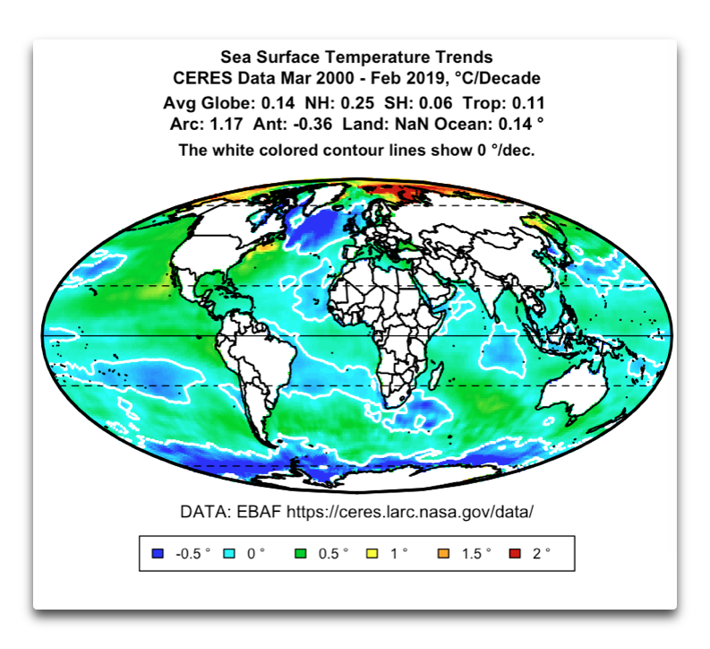
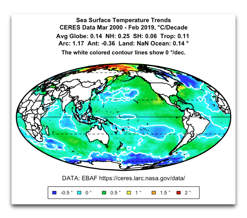
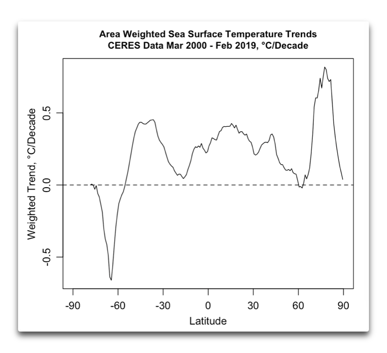
I’m sure you can see the difficulties …
w.
Cool, thanks Willis. I’m working on area weighted averages now. I’ll see how they compare.
From the article: “Probably the full ocean SST is increasing slightly, at the unremarkable rate of about 1.6°C/century. This shows up in the anomalies and in the ERSST plot. But this ignores the apparent complexity of the trend. The portion of the ocean with the best data is declining in temperature. Bottom line, we don’t know very much about what ocean temperatures are doing or where it is happening. Since the ocean temperature trend is the most important variable in detecting climate change, we don’t know much about climate change either. Nick was right that anomalies were able to pick out the probable trend, assuming that ERSST is correct, but by using anomalies important details were obscured.”
Saying “Probably the full ocean SST is increasing slightly” is just a guess.
You also say the *best data* shows a declining temperature trend. Why should we assume the ocean temperatures are increasing? Only because of computer manipulation of guesses.
We need to get away from computer simulations and get back to the actual data, if we want to know the truth, especially where it concerns climate science, since we know the “Keepers of the Flame” tend to make unwarranted warming assumptions about the atmosphere and oceans.
They always seem to find warming wherever they look. But they only look in their computers, not in the actual data. Computers are subject to dishonest manipulation, don’t you know. A common practice in the alarmist climate science world.
Let’s go with the real data and eliminate any computer dishonesty.
Tom, excellent points!
There are many many many things that can cause the oceans to warm, and CO2/LWIR of peak 15 microns ain’t one of them. How do I know that? Because CO2 used to be 7,000 PPM and the oceans didn’t boil away, life thrived. Visible radiation warms the oceans, not LWIR. If the oceans are warming, you have to determine if more incoming visible radiation is reaching the oceans. Simply go to WoodforTrees.org and look up cloud cover and guess what you will find? Sure enough, cloud cover has been decreasing for years. Fewer clouds, warmer oceans, CO2 has nothing to do with it.
More on exposing the AGW Fraud:
https://youtu.be/ZUVqZKBMF7o
Claiming that “on average”, the US has enough weather stations distorts the reality of the data.
The reality is that the vast majority of the sensors in the US are concentrated on the east coast and around the big cities on the west coast. Even in the interior most stations are clustered around the larger cities. There are vast areas of the US where there are simply not enough stations.
I’m know I’m way behind on this, but “anomaly” means a departure from normal. Who defined normal and how did they go about it?
They take temperatures from some baseline period, all with significant uncertainty intervals, average them all together, and assume the resultant average is 100% accurate as a baseline with no uncertainty. They then define that average as the normal.
They then use the normal to calculate the “anomaly”. They take independent, uncorrelated daily temps, average them, and call it a daily average. They then take the the daily averages and calculate a monthly average. They then take the monthly averages and average them to create an annual average.
At each step the uncertainty in the calculated result grows by leaps and bounds. But the climate scientists choose to ignore the uncertainty in their results and assume the averages are 100% accurate, infinitely precise, and actually represent something meaningful as a “normal”.
If I had tried this in one of my EE classes the professors would have had a conniption fit!
Tim, you say that “At each step the uncertainty in the calculated result grows by leaps and bounds.”
This is generally not true.
The general formula for the error of the mean of X, which has N data points and each error has a different value e, is
max(sem(x), weighted.mean(e))
where “sem” is the standard error of the mean.
In other words, if the values are widespread and the errors are small, the error of the mean is the standard error of the mean, which is std_dev(x)/sqrt(N).
But if the errors are large compared to the spread of the data, then the error of the mean is the weighted mean of the individual errors, weighted by their size.
Note that the uncertainty doesn’t “grow by leaps and bounds”.
w.
w,
“The general formula for the error of the mean of X, which has N data points and each error has a different value e, is”
There are no N data points. There is ONE data point for each temperature measurement. So there is no error of the mean.
You are making the common mistake of equating error and uncertainty.
Everything you say has to do with error and not uncertainty. Error is something that happens when you measure the same measurand using the same measurement device multiple times. The measurements make up a data set whose differences are random and make up a probability distribution. Look at the phrase you used: “and the errors are small”.
When you go out in the backyard and read your thermometer exactly how do you take multiple measurements of the same measurand? By the time you read it a s second time what the thermometer is indicating is the temperature of a different measurand since time has move on. You wind up with two independent measurements each with a set size of one. There is no probability distribution from which a mean can be calculated, there is no small error.
There *is*, however, still a systemic uncertainty for each measurement. That systemic uncertainty has no probability distribution. You simply don’t know where in that uncertainty interval the true value might lie. There is no “most probable” value. Therefore statistics can’t help you. Yet that systemic uncertainty still exists. And when you combine independent populations (of size 1) that are uncorrelated the uncertainties add as root sum square.
I should probably note that root sum square (i.e. adding in quadrature) is used instead of a direct sum of uncertainties becayse some true values will be above the indicated value and some will be below the indicated value. Thus a direct addition will probably overstate the combined uncertainty. But this is *not* the same thing as random errors cancelling out in a probability distribution.
Tim, you also say:
Mmm … kinda true. For most purposes, you can take an anomaly around any value and it makes no difference. For example, kelvins are an anomaly around absolute zero. Celsius is an anomaly around 273.15 kelvin, which is the freezing point of water.
Note that if the units are the same, such as one kelvin = 1° C, it generally doesn’t matter where you take the anomaly from. You could invent a new scale which is an anomaly around 100 K, with units of 1K, and use it for a host of purposes.
For example, if the temperature of an object goes from 273.15 K to 274.15 K, the change is 1 K. And the same is true when you use an anomaly around 273.15, such as the celsius scale. Using that scale, the temperature goes from 0°C to 1°C, which is 1°C = 1kelvin. So the anomaly and the absolute value give the same answer.
HOWEVER, if you want to use percentages, like a percentage increase in temperature, you have to use kelvin. This becomes important in thermodynamic where you are looking at things like say the efficiency of a heat engine.
Best regards,
w.
Of course it matters. An anomaly of 2degK at 100degK is far more significant than an anomaly of 2degK at 200degK. The first is a 2% change and the second is a 1% change.
When you use anomalies you hide the significance of the individual anomalies. That’s true even for Kelvin.
Tim, I just said immediately above your comment:
The kelvin scale is NOT an anomaly. It is an absolute temperature.
In response, you’ve come to tell us all that you can’t use anomalies for temperature increases …
w.
Measurement of temperature in Kelvins *is* an anomaly by definition. It is the anomaly from absolute zero that a Kelvin temperature represents.
Nor did I say that you can’t use anomalies for temperature increases. I *said* you can’t compare the impact of anomalies without knowing the base temperature. Nor can you determine anomalies from an artificial baseline (i.e. an average temperture) unless the uncertainty interval for that average is also provided. If the uncertainty interval for the average is large enough it will mask any anomaly calculation.
If your baseline has a value of 20C with an uncertainty of +/- 30C then you truly don’t know if an anomaly of 10C (i..e from 20C to 30C) is actually a true value or not. It could actually be a -20C anomaly and you wouldn’t know!
20C + 30C = 50C
20C – 30C = -10C
That’s a hell of a wide band. It’s going to mask a *lot* of anomalies!
I’ve attached an image showing my math concerning uncertainty and temperature. Hope it show up ok. I’ve not had anyone yet show me where the math is wrong.
Andy, here’s an example of how useful readings turn into confusion when you plot anomalies….
Hilarious and so true!
DMac, that is NOT an anomaly as they are usually defined. Seems like what you’ve done is average things month by month, and used that average as the baseline that you are taking the anomaly anomaly around … but if that’s the case, the mean for each month should be at zero, and the anomalies should be both positive and negative.
If you do it properly, with the monthly means set to zero, you don’t get the result in your second plot. Instead, you can see how much the variation is around the baseline for each month, and it will make much more sense.
w.
Where is the Greenhouse Gas-Powered Cars? If IR back radiation can warm the oceans, they can power engines. Where are the GHG Powered Cars? The structure would be simple and similar to a Sterling Engine.
1) Cylinder with an IR Transparent Compression Zone
2) Cylinder with an IR Absorptive Expansion Zone
CO2 would be compressed and exposed to LWIR back-radiation.
The CO2 would expand, pushing the Piston, and expanding in Volumn (PV/T).
The CO2 expands into the IR absorptive area, cooling and contracting.
The Piston cycles and compresses the CO2 into the area of the cylinder that is exposed to LWIR Back radiation.
The compressed CO2 absorbs the LWIR back radiation and expands.
The cycle repeated over and over and over again to form the world’s first perpetual motion machine.
If the LWIR can warm oceans, why can’t we use that energy to power cars?
CO2islife, once again your lack of knowledge of the subject matter betrays you.
A heat engine needs two things—a hot end and a cold end. Obviously, the hot end must be warmer than the cold end …
Now consider the downwelling radiation. It’s at something like 340 W/m2, which corresponds to a temperature of 5°C, much cooler than the average surface temperature of ~ 15° or so … but that’s the average.
When the surface is warmer, the downwelling radiation is warmer. In the tropics the average is 403 W/m2, or about 17°C.
At the poles it is 289 W/m2, or about -6 °C. The crucial point is, downwelling IR is always from a layer that is colder than the ground.
And that’s the problem … what are you going to use for the cold end of your heat engine, when the surroundings are always hotter than the hot end of your heat engine?
Note that such a setup would work fine in outer space. The earth radiates LWIR, which would warm the hot end of your heat engine. And at the cold end, the heat would readily escape to outer space.
But here on the surface? Not happening, for the reason listed above—no cold sink to dump the energy into.
And that, my friend, is why LWIR can’t power cars.
The Humboldt current flowing from Antarctica along the east coast of South America is the coldest it has been over the whole Holocene.
https://agupubs.onlinelibrary.wiley.com/doi/abs/10.1029/2018GL080634
Phil, I think you mean the eastern Pacific off the coast of western South America, but thanks for pointing out a very interesting paper.
Ocean temperatures show a lot of up and down fluctuation on century-millenial scale over the Holocene. This greatly reduces the significance of measurement of oceanic warming of a degree or two per century. It’s always doing that. It’s 50-50 that it will be warming or cooling at any time.
https://www.researchgate.net/profile/I_Mccave/publication/200032692_Holocene_periodicity_in_North_Atlantic_climate_and_deep-ocean_flow_south_of_Iceland/links/0c96052a70a1664e15000000/Holocene-periodicity-in-North-Atlantic-climate-and-deep-ocean-flow-south-of-Iceland.pdf
Andy,
<i>” there are so many weather stations, that arguably, gridding is unnecessary”</i>
No, that’s wrong. Gridding is not to compensate for lack of coverage. It is to link the sample of stations that you have with the area that they are supposed to represent. That is fundamental.
If you divide CONUS into two equal halves by area, one east one west, then the east has about twice as many stations as the west. That was true in V3, and V4, even though the latter has about ten times the number of stations. So a simple average over-represents the east. Now it isn’t obvious that one half is warmer than the other, so that might work about right, or not. It’s more obvious if you were averaging rainfall. You would definitely overstate the wetness of the US.
You can see how the arithmetic should work out thus. Suppose you had 1000 stations in the W, and 2000 in the E. If you had an average for the E and W, then a simple average would be right for CONUS. To get the W average, you would take each reading, divide by 1000 and add. To get the US average, each of those would have been multiplied by 1/2000. The E stations would initially have been multiplied by 1/2000 in the E average, and so by 1/4000 in the US. Overall, they are downweighted by 2, to compensate for their higher (2x) density.
If you just do a simple US average, each reading is multiplied by 1/3000 in the sum, and you’d get a different result. The key to getting a spatial integral, which is what you want here, is to weight each reading by inverse density. Gridding does that.
Nick,
Climate is determined by the entire temperature profile, maximum temps, minimum temps, and seasonal variations. Climate is *not* determined by an average, the average loses all data associated with the temperature profile. You can’t tell if maximum temps are impacting the average or if a specific impact comes from minimum temps. If you can’t determine even that simple discrimination then what good is the average?
I wish someone could clarify exactly what they think an average over a wide geographical area actually means. If you look at all the predictions based on the “global average temperature” that are abject failures you would think that someone, somewhere would start asking questions about the GAT.
<i>”Climate is *not* determined by an average”</i>
No-one said it was. But the average is the summary statistic used by scientists and laymen alike.
So what if it is the summary statistic used by SOME scientists and laymen? That doesn’t make it meaningful.
You failed to answer what you think a GAT actually means. You just used another False Appeal to Authority argumentative fallacy to justify its use. Pathetic.
Tim, for what GAT means, see The Elusive Absolute Surface Air Temperature.
w.
“The reason to work with anomalies, rather than absolute temperature is that absolute temperature varies markedly in short distances, while monthly or annual temperature anomalies are representative of a much larger region. Indeed, we have shown (Hansen and Lebedeff, 1987) that temperature anomalies are strongly correlated out to distances of the order of 1000 km.”
I’m sorry but this is crap. Kansas City to Denver is about 1000km. KC to St. Paul is about 650km. KC to Houston is about 1000km.
All of these cities have vastly different climates and their temperatures and temperature anomalies are not correlated very strongly at all. The most you can say is that they are all colder in winter and warmer in summer. How much colder each location is in winter compared to the others and how much warmer each location is in summer compared to the others is quite different.
And I will repeat once again, unless uncertainties are propagated while calculating monthly and annual averages there is no way to tell whether or not the difference in the anomalies are inside or outside the uncertainty interval. In other words without the uncertainty analysis you simply don’t know if there is a true trend or not.
Here’s the correlation of Kansas City, Denver, St. Paul, and Houston after removing seasonal variations:
St. Paul Denver KC Houston
St. Paul 1.00 0.73 0.89 0.30
Denver 0.73 1.00 0.66 0.21
Kansas City 0.89 0.66 1.00 0.20
Houston 0.30 0.21 0.20 1.00
(Have I said how much I dislike this new format? Does anyone know how to insert a clean table into a comment? Looks perfect when I type it, goes to Hades when I publish the comment. Grrrr…)
Per Hansen & Lebedeff 1987, the correlation at that distance averages about 0.6, with a minimum of 0.2 and a max of about 0.9.
And regarding the outlier, Houston, it is on the ocean and the rest are not. So we’d expect the correlations to be lower.
So your claim that “How much colder each location is in winter compared to the others and how much warmer each location is in summer compared to the others is quite different” is generally not true. Take a look at the cited reference for an extensive discussion.
However, I agree that the uncertainties should be included in each of these. The standard uncertainty of the means, the means which are subtracted to make the anomalies, is on the order of ±0.2°C to ±0.4°C. The range of the resulting anomalies is about -0.6 to +0.6. So the uncertainty is about half the range of the data … no bueno.
Regards,
w.
w.
I’m not sure what you think the correlation tells you. Correlation only tells you the direction and magnitude of how two variables vary.
So what? The stock price of Tesla and Chik-fil-a show a high level of correlation over the past decade. It doesn’t mean the stock prices of each are related in any way. Daily temps go up in the day and go down at night at all four locations, so they are highly correlated. So what? It doesn’t tell you what the relation between the four locations actually is.
And why take out the seasonal variation? Seasonal variation is a prime factor in a locations climate!
If you look at the USDA Hardiness Zone map KC is in Zone 6, St. Paul is in Zone 3, Denver in Zone 5, and Houston is in Zone 10. This is an indication of significant variation in climate. St Paul starts to cool off in the fall a full month before Kansas City does and KC cools off a full month before Houston does. KC has a longer growing season than St.Pal and a shorter one than Houston. The tomato growing season in St Paul is 3 months long, it is 6 months long in KC, and it is 8 months long in Houston. St Paul has a growing season barely long enough to get one crop of tomatoes. KC handles one crop easily and in Houston you can get two crops of tomatoes.
If you want to talk about correlation then consider that correlation = Cov(x,y)/sqrt[(var_x)(var_y). So let’s talk about Covariance. The maximum temperature at two locations comprises two populations of size 1. Each temperature is independent since it involves a different measurand and a different measurement device.
Cov(x,y) = sum [(x_i – u)(y_j – v)]/(size of the population)
u and v are the means of the population. For a population size of one the mean is the stated value in the population. So you wind up with sum[ (u -u)(v-v)] equals zero. This means the covariance is zero so the correlation of the two maximum temperatures is also zero. The same thing applies for minimum temperatures.
So daily averages using max and min temperatures consist of two unrelated maximum temps and two unrelated minimum temps. So how can the two average temps be related if the members are not related?
Please note that the terms in the calculation of covariance are ANOMALIES. Data points minus the mean is the definition of an anomaly.
Let me relate a story I was once given about analyzing independent populations. A rich philanthropist decides he’s going to buy new shirts for a tribe of pygmies and a tribe of Watusis in Africa. So he goes there and he measures the neck sizes of 1000 pygmies and 1000 Watusis. He then calculates the covariance for each and they both have a variance from -2 in to +2 in from the mean and the correlation of the anomalies is high. Same probability curve for both. So he says they must be related and he adds both populations together and calculates their mean. He then orders 2000 shirts with a neck size equal to the mean. When he starts handing them out he finds that they are too big for almost all of the pygmies and that they are too small for almost all of the Watusis. What????
The morals of the story are that it is difficult to combine independent populations and have the mean tell you anything and that the use of anomalies in statistics hide the underlying data. And it is the underlying data that is the most important to analyze, not the anomalies.
Temperatures in St Paul and Kansas City may have the same anomaly while having vastly different climates. Who knew?
(PS sorry to be so long in replying. Someone dug up my IP’s fiber cable with a backhoe and it took 14 hours yesterday to get service back!)
Thanks, Tim. You say:
In this case we’re looking at how correlation varies with distance. The closer two stations are, the more they are correlated.
This allows us to see, inter alia, if a particular station is way out of whack.
We’re not interested in a station’s climate. We’re interested in seeing if, when station A is warmer than normal for station A, it is also warmer for station B. Leaving in the seasonal variations prevents us from measuring that, since as you point out, the correlation of the raw data will be very high.
You continue:
And yet the correlation between them is high … go figure. You go on:
You are looking at a single data point at each location and talking about the correlation between two data points … I have no clue what this means.
Where in any of what I said did I discuss a “probability curve”? The probability curve of any random variable, from neck size to the throw of dice, will be quite similar, a “normal” bell-shaped distribution. Only a fool would conclude that because dice and neck sizes are randomly distributed, that their average is either possible or youthful.
In your philanthropist was smart, he would line up the two populations randomly, and take the correlation between the two lists of neck sizes, one for the Watusi, and one for the pygmies.
And when he saw there was no correlation between the two, whether he used absolute or anomalies of neck sizes, he’d avoid ordering shirts on that basis.
Look, I understand that if you take an average of the world population, each person has one breast and one testicle … but anyone designing brassieres is in for a rude shock. All your story shows is, play stupid games, win stupid prizes …
You close by saying:
In some cases we want to look at the underlying data, and in some cases we want to look at the anomalies. In some cases we want monthly anomalies. In other cases we want annual anomalies. In some cases we use raw data. There are no general rules for this. Which one we use is up to the details of the individual situation.
Apparently, everyone but you … and because of that, we can use their anomalies to find out important information about the climate.
My best regards and Christmas wishes, sorry to hear about the backhoe.
w.
“In this case we’re looking at how correlation varies with distance. The closer two stations are, the more they are correlated.”
Then why is Denver more highly correlated with St Paul (680 air miles) than with KC (550 air miles)? Perhaps there are confounding factors that aren’t being considered?
“We’re not interested in a station’s climate”
Of course we are. That’s the “climate change” agenda in a nutshell.
“And yet the correlation between them is high … go figure. You go on:”
The correlation is not between stations, the correlation is daily temperature rise/fall and seasonal rise/fall.
“You are looking at a single data point at each location and talking about the correlation between two data points … I have no clue what this means.”
Because that’s how you calculate the daily average temperature, two data points that are independent populations of size one whose covariance is zero. A single maximum data point at each location and a single minimum data point at each location. Then the monthly averages are based on the maximum/minimum temperature populations (populations of size one) as well. It’s independent populations of size one all the way down. If the base is uncorrelated then anything calculated from that base is uncorrelated also.
“Where in any of what I said did I discuss a “probability curve”? The probability curve of any random variable, from neck size to the throw of dice, will be quite similar, a “normal” bell-shaped distribution. Only a fool would conclude that because dice and neck sizes are randomly distributed, that their average is either possible or youthful.”
Please think about what you just said. When you take multiple temperature data points to create a data set with a population size greater than one they you are creating a probability distribution. If you don’t have a probability distribution then you can’t use probability statistics to analyze the data. And not all random variables produce a bell-shaped curve. The number of adults in households across the US is a skewed random variable, not a Gaussian random variable.
“take the correlation between the two lists of neck sizes, one for the Watusi, and one for the pygmies.”
That’s the issue. The covariance between the populations would be high because covariance is calculated based on the anomalies across the populations. If the variance of the anomalies for the two populations are similar then you get a high value for covariance. And such a situation is quite likely. Neck sizes for the two populations might turn out to be -2″ from the mean to +2″ from the mean. I.e. a range of 4″ in neck size for both. But that tells you nothing about what the actual shirts for each population should be. And correlation would be the same since it is directly calculated from the covariance.
“And when he saw there was no correlation between the two, whether he used absolute or anomalies of neck sizes, he’d avoid ordering shirts on that basis.”
You don’t calculate correlation based on absolute values, you calculate it based on anomalies. And there would be a high liklihood of significant correlation.
“In some cases we want to look at the underlying data, and in some cases we want to look at the anomalies. In some cases we want monthly anomalies. In other cases we want annual anomalies. In some cases we use raw data. There are no general rules for this. Which one we use is up to the details of the individual situation.”
We aren’t talking about “some cases”. We are talking about temperature and climate. Anomalies hide what is actually happening with the temperature and the climate. It’s why St Paul can have the exact same size of temperature anomaly as KC while having a far different climate.
“Apparently, everyone but you … and because of that, we can use their anomalies to find out important information about the climate.”
You can use the anomalies in St Paul to gain important information about the climate in ST PAUL. But they are meaningless for telling you about the climate in Kansas City. Because the climates in each location *are* different even if they have the same local anomalies.
You have a Merry Christmas as well and a safe 2021.
Tim Gorman
December 23, 2020 7:08 pm
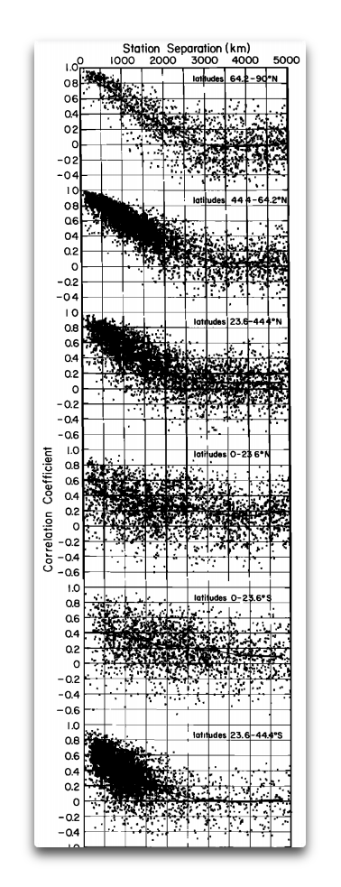
My apologies. I foolishly assumed you’d read the paper I pointed to above and looked at the graphs. They show that ON AVERAGE correlation varies with distance. The paper, assuming you’re still interested, is Hansen and Lebedeff 1987. Here is the graph in question:
But you and I haven’t been discussing climate. We were discussing the variation of correlation with station distance. Climate is a separate question, one for which that correlation is of interest.
Huh? This is perplexing. We seem to be having totally different discussions. I have said NOTHING about a correlation between daily and seasonal temperatures.
Again we seem to be having different discussions. A data point is ONE value, say the March temperature in San Francisco.
Another data point might be the March temperature in Portland. Note that each of these is a single number.
And we cannot measure a correlation between two individual numbers.
Now, if we have a bunch of months of San Franciso data, that is not a “data point”. It is a dataset. And we can find the correlation between that dataset and the corresponding Portland dataset.
Nitpick much? Do you think I don’t know about Poisson or Exponential or Uniform or LogNormal or Binomial distributions? Obviously, by “random variables” plus my description, I’m discussing random normal variables. I even said so, a “normal bell-shaped distribution”.
And you come back to school me on how not all variables don’t have a bell-shaped curve? This stuff is my meat and potatoes.
And you didn’t even deal with my point. The point of your story was that the explorer assumed that because two distributions have the same shape, we can average them together. I then pointed out that the explorer was an idiot. The example I gave was that the distributions of neck sizes and dice throws are both random normal (to avoid nitpicking), that does NOT mean that they can be averaged. How about you deal with that?
OK. I give up. It’s clear you don’t know what you are talking about. Here’s an example.
Suppose we have two temperature records in °F for one week. One of the datasets, we’ll call it V1, is, say, 55, 58, 60, 72, 65, 68, 62.
The other dataset, V2, is say 42, 46, 50, 59, 58, 65, 69.
The correlation of V1 and V2, the raw data, is 0.688.
Now, let’s take the anomalies of each one around the mean of each dataset. This gives us two new anomaly datasets, viz:
V3 = -7.86, -4.86, -2.86, 9.14, 2.14, 5.14, -0.86
V4 = -13.57, -9.57, -5.57, 3.43, 2.43, 9.43, 13.43
The correlation of V3 and V4, the anomaly datasets? It’s 0.688, the same as the correlation of the raw data.
How about the correlation between one absolute dataset and one anomaly dataset, say V1 and V4?
0.688, just like before.
How about if we change one of them to °C? Say
V5 = V1 in °C = 12.78, 14.44, 15.56, 22.22, 18.33, 20, 16.67
And the correlation between V5 (V1 in °C) and V2 (°F)?
0.688 …
OK, how about the correlation between the raw data in °C (V5) and the anomaly of the raw data in °F (V4)?
0.688.
Are we seeing a pattern here? Because I am.
The pattern is that you make flat statements about the most basic of mathematical operations, like …
“You don’t calculate correlation based on absolute values, you calculate it based on anomalies.”
… that are 100% demonstrably wrong, and then you defend them.
Sorry … not interested. Get a statistics textbook and learn about fundamental things like correlation, because it’s clear that you won’t let me teach you anything, and I’m unwilling to argue with you about whether a “normal” distribution is Gaussian, whether the correlation of anomalies and raw data is different, or whether a data point is the same as a dataset.
I regret having to do this, but life is too short for that kind of thing.
My best Xmas wishes to you and yours,
w.
“They show that ON AVERAGE correlation varies with distance.”
I simply don’t buy that unless their correlation definition is different than mine.
Oklahoma City is closer to KC than either Denver or St Paul. Yet Ok City’s temperatures aren’t correlated at all to those in KC. In fact Ok City very seldom sees freezing ice or snow on the roads while KC sees it all the time. Ok Cit doesn’t even keep a big fleet of snowplows or de-icing spreaders. Lincoln, NE is only 150 miles from KC yet Lincoln gets 5″ more of snow per year than does KC because of the differences in temperatures and weather fronts.
Lincoln averages 1650 heating degree-days per year (40degF set point) while KC, Mo only averages 1000 heating degree-days. That alone should tell you that there is a large difference in the temperatures in those two locations only 150mi apart. Denver averages 1300 heating degree-days St Paul averages 2400 heating degree-days per year. BTW, Ok City only averages 500 heating degree-days per year. St Louis, about the same latitude as KC and Denver, has only 800 heating degree-days per year.
Denver is much further away from KC than is Lincoln but KC the temperature profile is much closer to Denver’s than it is to Lincoln. St Louis has about 800 heating degree-days despite being on the same latitude as KC and Denver. Des Moines, IA has 1600 heating degree-days per year and is about 150 miles from Lincoln.
The article you referred to states: “ no substantial dependence on direction was found”
And, yet, there seems to be a *big* difference based on direction, at least where it concerns the central plains of the US.
The article also states: “The essence of the method which we use is shown schematically in Figure 5 for two nearby stations, for which we want the best estimate of the temperature change in their mutual locale. We calculate the mean of both records for the period in common, and adjust the entire second record (T2) by the difference (bias) ST. The mean of the resulting temperature records is the estimated temperature change as a function of time. The zero point of the temperature scale is arbitrary. ” (bolding mine, tpg)
So, once again, we see the use of AVERAGES and means to try and compare temperatures between different localities. This really isn’t much different than what we see so many climate scientists (such as Stokes) doing today.
This simply does not provide a good indication of what is going on where. Which is why I see heating/cooling degree-days as a much better tool to use for comparisons. The heating/cooling degree days are an integral of the entire temperature profile at a location. Higher temperatures drive higher cooling degree-days and colder temperatures drive higher heating degree-days. It’s why Anchorage, AK temperatures (2600 heating degree-days) correlates better with St Paul than KC or Denver even though the distance is far larger. The temperature profile, which is what determines climate, is closer between Anchorage and St. Paul then St. Paul and KC.
w,
“ How about you deal with that?”
I don’t deal with that. The two distributions are HIGHLY correlated. That doesn’t mean they are the same. It’s exactly like temperatures. Temperature change over time follows a sine curve in most places. That means that the resulting temperatures will turn out to be highly correlated if you only look at the anomalies from the mean. That does *not* mean that the temperature distribution between two locations are the same.That’s why heating/cooling degree-days, which does not depend on anomalies, is a far better tool to use in analyzing what is going on where.
Tim, perhaps you didn’t read to the end of my last post, or you thought I wasn’t serious when I said:
I was perfectly serious. You don’t know the math well enough to realize that correlations are the same whether you use absolute values or anomalies, and that level of mathematic ignorance is more than I can handle … particularly because when I point out your errors, you either ignore me or you defend your foolish mistakes.
Get a college statistics textbook, read it end to end, and we’ll talk again.
Best Christmas wishes,
w.
So much to unpack here. My key point in this series of posts, is that all the massaging of the data, including making anomalies, corrections, bias-corrections, averaging, gridding, is making the result “look better” than it actually is. This massaging vastly oversimplifies and gives the public and climate scientists more confidence than they should have. William Briggs may have said it best in a post referenced above by Geoff Sherrington. The post is about smoothing, but I took it to mean all methods of massaging data.
https://wmbriggs.com/post/195/
Gridding helps to define dominant internal trends in mapped areas. Anomalies help identify and project trends, but both remove information and complexity. Both can be and are misleading – they also oversimplify. Present them if you wish, but also show the real measurements.
“He [Nick Stokes] believes the measured temperatures are showing cooling because the coverage of cold regions is improving over time and this creates an artificial cooling trend.”
Interesting that he says the opposite in regard to increasing metropolitan temperatures while the countryside temperatures do not reflect any concern for worry.
My problem is that even if 15 um could heat the ocean, the heat capacity of CO2 is so small compared to the ocean that one could compare it to a 100 watt bulb heating a covered NFL stadium.
Jim, downwelling IR is about 345 W/m2.
A 100 watt light bulb irradiating an NFL stadium? Well, the field is ~ 100m x 50m, or 5000 m2. As a result, just for the field and ignoring the rest of the stadium, downwelling radiation from the light bulb (assuming a perfect reflector above it so no radiation at any frequency goes upwards) is already only 100 / (100 * 50) = 1/50 = 0.02 W/m2 …
So no, one cannot compare the two as you suggest.
My advice?
Pay no attention to CO2islife, he’ll lead you wrong every time. Instead, read my post entitled “Radiating The Ocean“.
w.