By Hartmut Hoecht
1. Introduction
This paper addresses the glaring disregard within the scientific community in addressing thermal data errors of global ocean probing. Recent and older records are compiled with temperatures noted in small fractions of degrees, while their collection processes often provide errors much greater than full degrees. As a result of coarse methods the very underpinning of the historic and validity of the present database is questioned, as well as the all-important global temperature predictions for the future.
Follow me into the exploration of how the global ocean temperature record has been collected.
First, a point of reference for further discussion:
Wikipedia, sourced from NASA Goddard, has an illustrative graph of global temperatures with an overlay of five-year averaging. Focus on the cooling period between mid 1940’s and mid 1970’s. One can glean the rapid onset of the cooling, which amounted to approximately 0.3 degree C in 1945, and its later clearly discernible reversal.

The May 2008 paper by Thompson et al in Nature got my attention. Gavin Schmidt of RealClimate and also the New Scientist commented on it. Thompson claims he found the reason why the 1940’s cooling started with such a drastic reversal from the previous heating trend, something that apparently had puzzled scientists for a long time. The reason for this flip in temperature was given as the changeover in methods in collecting ocean temperature data. That is, changing the practice of dipping sampling buckets to reading engine cooling water inlet temperatures.
Let us look closer at this cooling period.
Before and after WWII the British fleet used the ‘bucket method’ to gather ocean water for measuring its temperature. That is, a bucket full of water was sampled with a bulb thermometer. The other prevalent probing method was reading ships’ cooling water inlet temperatures.
These two data gathering methods are explained in a 2008 letter to Nature, where Thompson et al coined the following wording (SST = sea surface temperature):
“The most notable change in the SST archive following December 1941 occurred in August 1945. Between January 1942 and August 1945 ~80% of the observations are from ships of US origin and ~5% are from ships of UK origin; between late 1945 and 1949 only ~30% of the observations are of US origin and about 50% are of UK origin. The change in country of origin in August 1945 is important for two reasons: first, in August 1945 US ships relied mainly on engine room intake measurements whereas UK ships used primarily uninsulated bucket measurements, and second, engine room intake measurements are generally biased warm relative to uninsulated bucket measurements.”
Climate watchers had detected a bump in the delta between water and night time atmospheric temperatures (NMAT). Therefore it was thought that they had found the culprit for the unexplained 0.3 degree C flip in temperatures around 1945, which invited them to tweak and modify the records. The applied bias corrections, according to Thompson, “might increase the century-long trends by raising recent SSTs as much as ~0.1 deg. C”.
Supposedly this bias correction was prominently featured in the IPCC 2007 summary for policy makers. The question to ask – how was Thompson’s 0.1 degree correction applied – uniformly? Over what time period? Is the number of 0.1 degree a guess and arbitrarily picked? Does it account for any measurement errors, those discussed further in this paper?
A fundamental question arises how authentic is our temperature record? How confidently can we establish trend lines and future scenarios? It is obvious that we need to know the numbers within 0.1 degree C accuracy to allow sensible interpretation of the records and to believably project future global temperatures.
We shall examine the methods of measuring ocean water temperatures in detail, and we will discover that the data record is very coarse, often by much more than an order of magnitude!
First, it is prudent to present the fundamentals, in order to establish a common understanding.
2. The basics
We can probably agree that, for extracting definite trends from global temperature data, the resolution of this data should be at least within +/-0.1 degree C. An old rule of thumb for any measurement cites the instrument having better than three times the accuracy of the targeted resolution. In our case it is +/0.03 degree C.
Thermal instrument characteristics define error in percent of full range. Read-out resolution is another error, as is read-out error. Example: assume a thermometer has a range of 200 degrees , 2 % accuracy is 4 degrees, gradation (resolution) is 2 degrees. Read-out accuracy may be 0.5 degrees, to be discerned between gradations, if you ‘squint properly’.
Now let us turn to the instruments themselves.
Temperature is directly measured via bulb and capillary function liquid based thermometers, bimetal dial gages and, with the help of electronics, the thermistors, as well as a few specialized methods. Via satellite earth temperatures are interpreted indirectly from infrared radiative reflection.
We are all familiar with the capillary and liquid filled thermometers we encounter daily. They and bimetal based ones have typical accuracy of +/-1 to 2 percent and are no more accurate than to 0.5 degree C. The thermistors can be highly accurate upon precise calibration.
Temperature data collection out in nature focuses not just on the thermal reading device by itself. It is always a system, which comprises to various extent the data collection method, temporary data storage, data conversion and transmission, manipulation, etc. Add to this the variations of time, location, of protocol, sensor drift and sensor deterioration, variations in the measured medium, different observers and interpreters, etc. All of this contributes to the system error. The individual error components are separated into the fixed known – errors and the random – variable errors. Further, we must pay attention to the ‘significant figures’ when assessing error contributors, since a false precision may creep in, when calculation total error.
Compilation of errors:
All errors identified as random errors are combined using the square root of the sum of the squares method (RSS). Systematic errors are combined by algebraic summation. The total inaccuracy is the algebraic sum of the total random error and total systematic error.
3. Predominant ocean temperature measuring methods
a. Satellite observations
Data gathering by infrared sensors on NOAA satellites has been measuring water surface temperatures with high-resolution radiometers.
Measurements are indirect and must take into account the uncertainties associated with other parameters, which can be only poorly estimated. Only the top-most water layer can be measured, which can induce a strong diurnal error. Satellite measurements came into use around the 1970’s, so they have no correlation to earlier thermal profiling. However, since they are indirect methods of reading ocean temperature and have many layers of correction and interpretation with unique error aspects, they are not investigated here. Such an effort would warrant a whole other detailed assessment.
b. Direct water temperature measurements – historical
Dipping of a thermometer in a bucket of a collected water sample was used prior to the need for understanding the thermal gradients down in deeper portions of the ocean. The latter became vital for submarine warfare, before and during WWII. Earlier, water temperature knowledge was needed only for meteorological forecasting.
The ‘Bucket Method’:
Typically a wooden bucket was thrown from a moving ship, hauled aboard, and a bulb thermometer was dipped in this bucket to get the reading. After the earlier wooden ones, canvas buckets became prevalent.

- depth of bucket immersion
- surface layer mixing from variable wave action and solar warming
- churning of surface layer from ship’s wake
- variable differential between water and air temperature
- relative direction between wind and ship’s movement
- magnitude of combined wind speed and ship’s speed
- time span between water collection and actual thermal readings
- time taken to permit thermometer taking on water temperature
- degree of thermometer stirring (or not)
- reading at the center vs. edge of the bucket
- thermometer wet bulb cooling during reading of temperature
- optical acuity and attitude of operator
- effectiveness of bucket insulation and evaporative cooling effects of leakage
- thermal exchange between deck surface and bucket
Here is an infrared sequence showing how water in a canvas bucket cools.

Figures above from this paper:
ABSTRACT: Uncertainty in the bias adjustments applied to historical sea-surface temperature (SST) measurements made using buckets are thought to make the largest contribution to uncertainty in global surface temperature trends. Measurements of the change in temperature of water samples in wooden and canvas buckets are compared with the predictions of models that have been used to estimate bias adjustments applied in widely used gridded analyses of SST. The results show that the models are broadly able to predict the dependence of the temperature change of the water over time on the thermal forcing and the bucket characteristics: volume and geometry; structure and material. Both the models and the observations indicate that the most important environmental parameter driving temperature biases in historical bucket measurements is the difference between the water and wet-bulb temperatures. However, assumptions inherent in the derivation of the models are likely to affect their applicability. We observed that the water sample needed to be vigorously stirred to agree with results from the model, which assumes well-mixed conditions. There were inconsistencies between the model results and previous measurements made in a wind tunnel in 1951. The model assumes non-turbulent incident flow and consequently predicts an approximately square-root dependence on airflow speed. The wind tunnel measurements, taken over a wide range of airflows, showed a much stronger dependence. In the presence of turbulence the heat transfer will increase with the turbulent intensity; for measurements made on ships the incident airflow is likely to be turbulent and the intensity of the turbulence is always unknown. Taken together, uncertainties due to the effects of turbulence and the assumption of well-mixed water samples are expected to be substantial and may represent the limiting factor for the direct application of these models to adjust historical SST observations.
Engine Inlet Temperature Readings:
A ship’s diesel engine uses a separate cooling loop, to isolate the metal from the corrosive and fouling effect of sea water. The raw water inlet temperature is most always measured via gage (typical 1 degree C accuracy and never recalibrated), which is installed between the inlet pump and the heat exchanger. There would not be a reason to install thermometers directly next to the hull without data skewing engine room heat-up, a location which would otherwise be more useful for research purposes.
Random measurement influences to be considered:
- depth of water inlet
- degree of surface layer mixing from wind and sun
- wake churning of ship, also depending on speed
- differential between water and engine room temperature
- variable engine room temperature
Further, there are long-term time variable system errors to be considered:
- added thermal energy input from the suction pump
- piping insulation degradation and from internal fouling.
c. Deployed XBT (Expendable Bathythermograph) Sondes
The sonar sounding measurements and the need for submarines hiding from detection in thermal inversion layers fueled the initial development and deployment of the XBT probes. They are launched from moving surface ships and submarines. Temperature data are sent to aboard the ship via unspooling of a thin copper wire from the probe, while it takes on a slightly decreasing descending speed. Temperature is read by a thermistor; processing and recording of data is done with shipboard instruments. The depth is calculated by the elapsed time, and based on a manufacturer’s specific formula. Thermistor readings are recorded via voltage changes of the signal.
Random errors introduced:
- thermal lag effect of probe shipboard storage vs. initial immersion temperature
- storage time induced calibration drift
- dynamic stress plus changing temperature effect on copper wire resistance during descent
- variable thermal lag effect on thermistor during descent
- variability of surface temperature vs. stability of deeper water layers
- instrument operator induced variability.
d. ARGO Floating Buoys
The concept of these submersed buoys is a clever approach to have nearly 4000 such devices worldwide autonomously recording water data, while drifting at different ocean depths. Periodically they surface and batch transmit the stored time, depth (and salinity) and temperature history via satellite to ground stations for interpretation. The prime purpose of ARGO is to establish a near-simultaneity of the fleet’s temperature readings down to 2500 meters in order to paint a comprehensive picture of the heat content of the oceans.
Surprisingly, the only accuracy data given by ARGO manufacturers is the high precision of 0.001 degree C of their calibrated thermistor. Queries with the ARGO program office revealed that they have no knowledge of a system error, an awareness one should certainly expect from this sophisticated scientific establishment. An inquiry about various errors with the predominant ARGO probe manufacturer remains unanswered.
In fact, the following random errors must be evaluated:
- valid time simultaneity in depth and temperature readings, since the floats move with currents and may transition into different circulation patterns, i.e. different vertical and lateral ones
- thermal lag effects
- invalid readings near the surface are eliminated; unknown extent of depth of the error
- error in batch transmissions from the satellite antenna due to wave action
- error in two-way transmissions, applicable to later model floats
- wave and spray interference with high frequency 20/30 GHz IRIDIUM satellite data transmission
- operator and recordation shortcomings and misinterpretation of data
Further, there are unknown resolution, processor and recording instrument systems errors, such as coarseness of the analog/digital conversion, any effects of aging float battery output, etc. Also, there are subtle characteristics between different float designs, which are probably hard to gage without detailed research.
e. Moored Ocean Buoys
Long term moored buoys have shortcomings in vertical range, which is limited by their need to be anchored, as well as in timeliness of readings and recordings. Further, they are subject to fouling and disrupted sensor function from marine biological flora. Their distribution is tied to near shore anchorage. This makes them of limited value for general ocean temperature surveying.
f. Conductivity, Temperature, Depth (CTD) Sondes
These sondes present the most accurate method of water temperature readings at various depths. They typically measure conductivity, temperature (also often salinity) and depth together. They are deployed from stationary research ships, which are equipped with a boom crane to lower and retrieve the instrumented sondes. Precise thermistor thermal data at known depths are transmitted in real-time via cable to onboard recorders. The sonde measurements are often used to calibrate other types of probes, such as XBT and ARGO, but the operational cost and sophistication as a research tool keeps them from being used on a wide basis.
4. Significant Error Contributions in Various Ocean Thermal Measurements
Here we attempt to assign typical operational errors to the above listed measuring methods.
a. The Bucket Method
Folland et al in the paper ‘Corrections of instrumental biases in historical sea surface temperature data’ Q.J.R. Metereol. Soc. 121 (1995) attempted to quantify the bucket method bias. The paper elaborates on the historic temperature records and variations in bucket types. Further, it is significant that no marine entity has ever followed any kind of protocol in collecting such data. The authors of this report undertake a very detailed heat transfer analysis and compare the results to some actual wind tunnel tests (uninsulated buckets cooling by 0.41 to 0.46 degree C). The data crunching included many global variables, as well as some engine inlet temperature readings. Folland’s corrections are +0.58 to 0.67 degree C for uninsulated buckets and +0.1 to 0.15 degrees for wooden ones.
Further, Folland et al (1995) state “The resulting globally and seasonally averaged sea surface temperature corrections increase from 0. 11 deg. C in 1856 to 0.42 deg. C by 1940.”
It is unclear why the 19th century corrections would be substantially smaller than those in the 20th century. Yet, that could be a conclusion from the earlier predominance of the use of wooden buckets (being effectively insulating). It is also puzzling, how these numbers correlate to Thompson’s generalizing statement that recent SSTs should be corrected via bias error “by as much as ~0.1 deg. C”? What about including the 0.42 degree number?
In considering a system error – see 3b. – the variable factors of predominant magnitude are diurnal, seasonal, sunshine and air cooling, spread of water vs. air temperature, plus a fixed error of thermometer accuracy of +/- 0.5 degree C, at best. Significantly, bucket filling happens no deeper than 0.5 m below water surface, hence, this water layer varies greatly in diurnal temperature.
Tabatha, 1978, says about measurement on a Canadian research ship – “bucket SSTs were found to be biased about 0.1°C warm, engine-intake SST was an order of magnitude more scattered than the other methods and biased 0.3°C warm”. So, here both methods measured warm bias, i.e. correction factors would need to be negative, even for the bucket method, which are the opposite of the Folland numbers.
Where to begin in assigning values to the random factors? It seems near impossible to simulate a valid averaging scenario. For illustration sake let us make an error calculation re. a specific temperature of the water surface with an uninsulated bucket.
Air cooling 0.50 degrees (random)
Deckside transfer 0.05 degrees (random)
Thermometer accuracy 1.0 degrees (fixed)
Read-out and parallax 0.2 degrees (random)
Error e = 1.0 + (0.52 + 0.052 + 0.22)1/2 = 1.54 degrees or 51 times the desired accuracy of 0.03 degrees (see also section 2.0).
b. Engine intake measurements
Saur 1963 concludes : “The average bias of reported sea water temperatures as compared to sea surface temperatures , with 95% confidence limits, is estimated t be 1.2 +/-0.6 deg F (0.67 +/-0.3 deg C) on the basis of of a sample of 12 ships. The standard deviation is estimated to be 1.6 deg F (0.9 deg C)….. The ship bias (average bias of injection temperatures from a given ship) ranges from -0.5 deg F to 3.0 deg F (0.3 deg C to 1.7 deg C) among 12 ships.”
Errors in engine-intake SST depend strongly on the operating conditions in the engine room (Tauber 1969).
James and Fox (1972) show that intakes at 7m depth or less showed a bias of 0.2 degree C and deeper inlets had biases of 0.6 degree C.
Walden, 1966, summarizes records from many ships as reading 0.3 degree C too warm. However, it is doubtful that accurate instrumentation was used to calibrate readings. Therefore, his 0.3 degree number is probably derived crudely with shipboard standard ½ or 1 degree accuracy thermometers.
Let us make an error calculation re. a specific water temperature at the hull intake.
Thermometer accuracy 1.0 degree (fixed)
Ambient engine room delta 0.5 degree (random)
Pump energy input 0.1 degree (fixed)
Total error 1.6 degree C or 53 times the desired accuracy of 0.03 degrees.
One condition of engine intake measurements that differs strongly from the bucket readings is the depth below water surface at which measurements are collected, i.e. several meters down from the surface. This method provides cooler and much more stable temperatures as compared to the buckets nipping water and skipping along the top surface. However, engine room temperature appears highly influential. Many records are only given in full degrees, which is the typical thermometer resolution.
But, again the only given fixed error is the thermometer accuracy of one degree, as well as the pump energy heating delta. The variable errors may be of significant magnitude on larger ships and they are hard to generalize.
All these wide variations makes the engine intake record nearly impossible to validate. Further, the record was collected at a time when research based calibration was hardly ever practiced.
c. XBT Sondes
Lockheed-Martin (Sippican) produces several versions, and they advertise temperature accuracy of +/- 0.1 degree C and a system accuracy of +/- 0.2 degree C. Aiken (1998) determined an error of +0.5 and in 2007 Gouretski found an average bias of +0.2 to 0.4 degree C. The research community also implies accuracy variations with different data acquisition and recording devices and recommends calibration via parallel CTD sondes. There is a significant variant in the depth – temperature correlation, about which the researchers still hold workshops to shed light on.
We can only make coarse assumptions for the total error. Given the manufacturer’s listed system error of 0.2 degrees and the range of errors as referenced above, we can pick a total error of, say, 0.4 degree C, which is 13 times the desired error of 0.03 degrees.
d. ARGO Floats
The primary US based float manufacturer APEX Teledyne boasts a +/-0.001 degree C accuracy, which is calibrated in the laboratory (degraded to 0.002 degrees with drift). They have confirmed this number after retrieving a few probes after several years of duty. However, there is no system accuracy given, and the manufacturer stays mum to inquiries. The author’s communication with the ARGO program office reveals that they don’t know the system accuracy. This means they know the thermistor accuracy and nothing beyond. The Seabird Scientific SBE temperature/salinity sensor suite is used within nearly all of the probes, but the company, upon email queries, does not reveal its error contribution. Nothing is known about the satellite link errors or the on-shore processing accuracies.
Hadfield (2007) reports a research ship transection at 36 degree North latitude with CTD measurements. They have compared them to ARGO float temperature data on both sides of the transect and they are registered within 30 days and sometimes beyond. Generally the data agree within 0.6 degree C RMS and a 0.4 degree C differential to the East and 2.0 degree to the West. These readings do not relate to the accuracy of the floats themselves, but relate to limited usefulness of the ARGO data, i.e. the time simultaneity and geographical location of overall ocean temperature readings. This uncertainty indicates significant limits for determining ocean heat content, which actually is the raison d’etre for ARGO.
The ARGO quality manual for CTD’s and transectory data does spell out the flagging of probably bad data. The temperature drift between two average values is to be max. 0.3 degrees as fail criterion, the mean at 0.02 and a minimum 0.001 degrees.
Assigning an error budget to ARGO float readings certainly means a much higher than the manufacturer’s stated value of 0.002 degrees.
So, let’s try:
Allocated system error 0.01 degree (assume fixed)
Data logger error and granularity 0.01 (fixed)
Batch data transmission 0.05 (random)
Ground based data granularity 0.05 (fixed)
Total error 0.12 degrees, which is four times the desired accuracy of 0.03 degrees.
However, the Hadfield correlation to CTD readings from a ship transect varies up to 2 degrees, which is attributable to time and geographic spread and some amount of ocean current flow and seasonal thermal change, in addition to the inherent float errors.
The NASA Willis 2003/5 ocean cooling episode:
This matter is further discussed in the summary section 5.
In 2006 Willis published a paper, which showed a brief ocean cooling period, based on ARGO float profile records.
“Researchers found the average temperature of the upper ocean increased by 0.09 degrees Celsius (0.16 degrees F) from 1993 to 2003, and then fell 0.03 degrees Celsius (0.055 degrees F) from 2003 to 2005. The recent decrease is a dip equal to about one-fifth of the heat gained by the ocean between 1955 and 2003.”
The 2007 paper correction tackles this apparent global cooling trend during 2003/4 by removing specific wrongly programmed (pressure related) ARGO floats and by correlating earlier warm biased XBT data, which, together, was said to substantially minimize the magnitude of this cooling event.
Willis’ primary focus was gaging the ocean heat content and the influences on sea level. The following are excerpts from his paper, with and without the correction text.
Before correction:
“The average uncertainty is about 0.01 °C at a given depth. The cooling signal is distributed over the water column with most depths experiencing some cooling. A small amount of cooling is observed at the surface, although much less than the cooling at depth. This result of surface cooling from 2003 to 2005 is consistent with global SST products [e.g. http://www.jisao.washington.edu/data_sets/global_sstanomts/]. The maximum cooling occurs at about 400 m and substantial cooling is still observed at 750 m. This pattern reflects the complicated superposition of regional warming and cooling patterns with different depth dependence, as well as the influence of ocean circulation changes and the associated heave of the thermocline.
The cooling signal is still strong at 750 m and appears to extend deeper (Figure 4). Indeed, preliminary estimates of 0 – 1400 m OHCA based on Argo data (not shown) show that additional cooling occurred between depths of 750 m and 1400 m.”
After correction:
“…. a flaw that caused temperature and salinity values to be associated with incorrect pressure values. The size of the pressure offset was dependent on float type, varied from profile to profile, and ranged from 2–5 db near the surface to 10–50 db at depths below about 400 db. Almost all of the WHOI FSI floats (287 instruments) and approximately half of the WHOI SBE floats (about 188 instruments) suffered from errors of this nature. The bulk of these floats were deployed in the Atlantic Ocean, where the spurious cooling was found. The cold bias is greater than −0.5°C between 400 and 700 m in the average over the affected data.
The 2% error in depth presented here is in good agreement with their findings for the period. The reason for the apparent cooling in the estimate that combines both XBT and Argo data (Fig. 4, thick dashed line) is the increasing ratio of Argo observations to XBT observations between 2003 and 2006. This changing ratio causes the combined estimate to exhibit cooling as it moves away from the warm-biased XBT data and toward the more neutral Argo values.
Systematic pressure errors have been identified in real-time temperature and salinity profiles from a small number of Argo floats. These errors were caused by problems with processing of the Argo data, and corrected versions of many of the affected profiles have been supplied by the float provider.
Here errors in the fall-rate equations are proposed to be the primary cause of the XBT warm bias. For the study period, XBT probes are found to assign temperatures to depths that are about 2% too deep.”
Note that Willis and co-authors estimated the heat content of the upper 750 meters. This zone represents about 20 percent of the global ocean’s average depth.
Further, the Fig. 2 given in Willis’ paper shows the thermal depth profile of one of the eliminated ARGO floats, i.e. correct vs. erroneous.

Averaging the error at specific depth we can glean a 0.15 degree differential, ranging from about 350 to 1100 m. That amount differs from the cold bias of -0.5 degree as stated above, albeit as defined within 400 and 700 meters.
All of these explanations by Willis are very confusing and don’t inspire confidence in any and all ARGO thermal measurement accuracies.
5. Observations and Summary
5.1 Ocean Temperature Record before 1960/70
Trying to extract an ocean heating record and trend lines during the times of bucket and early engine inlet readings seems a futile undertaking because of vast systematic and random data error distortion.
The bucket water readings were done for meteorological purposes only and
a. without quality protocols and with possibly marginal personnel qualification
b. by many nations, navies and merchant marine vessels
c. on separate oceans and often contained within trade routes
d. significantly, scooping up only from a thin surface layer
e. with instrumentation that was far cruder than the desired quality
f. subject to wide physical sampling variations and environmental perturbances
Engine inlet temperature data were equally coarse, due to
a. lack of quality controls and logging by marginally qualified operators
b. thermometers unsuitable for the needed accuracy
c. subject to broad disturbances from within the engine room
d. variations in the intake depth
e. and again, often confined to specific oceans and traffic routes
The engine inlet temperatures differed significantly from the uppermost surface readings,
a. being from a different depth layer
b. being more stable than the diurnally influenced and solar heated top layer
Observation #1:
During transition in primary ocean temperature measuring methods it appears logical to find an upset of the temperature record around WWII due to the changes in predominant method of temperature data collection. However, finding a specific correction factor for the data looks more like speculation, because the two historic collection methods are just too disparate in characteristics and in what they measure. This appears to be a case of the proverbial apples and oranges comparison. However, the fact of a rapid 1945/6 cooling onset must still be acknowledged, because the follow-on years remained cool. Then, the warming curve in the mid-seventies started again abruptly, as the graph in section 1 shows so distinctly.
5.2 More recent XBT and ARGO measurements:
Even though the XBT record is of limited accuracy, as reflected in a manufacturer’s stated system accuracy of +/- 0.2 degrees, we must recognize its advantages and disadvantages, especially in view of the ARGO record.
XBT data:
a. they go back to the 1960’s, with an extensive record
b. ongoing calibration to CBT measurements is required because the calculation depth formulae are not consistently accurate
c. XBT data are firm in simultaneous time and geographical origin, inviting statistical comparisons
d. recognized bias of depth readings, which are relatable to temperature
ARGO data:
a. useful quantity and distribution of float cycles exist only since around 2003
b. data accuracy cited as extremely high, but with unknown system accuracy
c. data collection can be referenced only to point in time of data transmission via satellite. Intermediary ocean current direction and thermal mixing during float cycles add to uncertainties.
d. calibration via CTD probing are hampered by geographical and time separation and have lead to temperature discrepancies of three orders of magnitude, i.e. 2.0 (Hadfield 2007) vs. 0.002 degrees (manufacturer’s statement)
e. programming errors have historically read faulty depth correlations
f. unknown satellite data transmission errors, possibly occurring with the 20/30 GHz frequency signal attenuation from wave action, spray and hard rain.
Observation#3:
The ARGO float data, despite the original intent on creating a precise ocean heat content map, must be recognized within its limitation. The ARGO community knows not the float temperature system error.
NASA’s Willis research on the 2003/4 ocean cooling investigation leaves open many questions:
a. is it feasible to broaden the validity of certain ARGO cooling readings from a portion of the Atlantic to the database of the entire global ocean?
b. is it credible to conclude that a correction to a small percentage of erroneous depth offset temperature profiles across a narrow vertical range has sufficient thermal impact on the mass of all the oceans, such as to claim global cooling or not?
c. Willis argues that the advent of precise ARGO readings around year 2003 vs. the earlier record of warm biased XBT triggered the apparent ocean cooling onset. However, this XBT warm bias was well known at that time. Could he not have accounted for this bias when comparing the before-after ARGO rise to prominence?
d. Why does the stated cold bias of -0.5 degree C given by Willis differ significantly from the 0.15 degree differential that can be seen in his graph?
Observation #4:
The subject Willis et al research appears to be an example of inappropriate mixing two different generic types of data (XBT and ARGO) and it concludes, surprisingly
a. the prior to 2003 record should be discounted for apparent cooling upset and
b. this prior to 2003 record should still be a valid one for determining the trend line of ocean heat content.
Willis states ”… surface cooling from 2003 to 2005 is consistent with global SST products” (SST = sea surface temperature). This statement contradicts the later conclusion that the cool-down was invalidated by the findings of his 2007 corrections.
Further, Willis’manipulation of float meta data together with XBT data is confusing enough to make one question his conclusions in the correction paper of 2007.
Summary observations:
- It appears that the historic record of ‘bucket’ and ‘engine inlet’ temperature record should be regarded as anecdotal, historic and overly coarse, rather than to serve the scientific search for ocean warming trends. With the advent of XBT and ARGO probes the trend lines read more accurately, but they are often obscured by instrument systems error.
- An attempt of establishing the ocean temperature trend must consider the magnitude of random errors vs. known system errors. If one tries to find a trend line in a high random error field the average value may find itself at the extreme of the error band, not at its center.
- Ocean temperature should be discernable to around 0.03 degrees C precision. However, system errors often exceed this precision by up to three orders of magnitude!
- If NASA’s Willis cited research is symptomatic for the oceanic science community in general, the supposed scientific due diligence in conducting analysis is not to be trusted.
- With the intense focus on statistical manipulation of meta data and of merely what’s on the computer display many scientists appear to avoid exercising due prudence in appropriately factoring in data origin for it accuracy and relevance. Often there is simply not enough background about the fidelity of raw data to make realistic estimates of error, and neither for drawing any conclusions as to whether the data is appropriate for what it is being used.
- Further, the basis of statistical averaging means averaging the same thing. Ocean temperature data averaging over time cannot combine averages from a record of widely varying data origin, instruments and methods. Their individual pedigree must be known and accounted for!
Lastly, a proposal:
Thompson, when identifying the WWII era temperature blip between bucket and engine inlet records, had correlated them to NMAT, i.e. the night time temperatures for each of the two collection methods. NMATs may be a way – probably to a limited degree – to validate and tie together the disparate record all the way from the 19th century to future satellite surveys.
This could be accomplished by research ship cruises into cold, temperate and hot ocean zones, measuring simultaneously, i.e. re. time and location, representative bucket and engine inlet temperatures and deploying a handful of XBT and ARGO sondes, while CBT probing at the same time. And all these processes are to be correlated under similar night time conditions and with localized satellite measurements. With this cross-calibration one could back trace the historical records and determine the delta temperatures to their NMATs, where such a match can be found. That way NMATs could be made the Rosetta Stone to validating old, recent and future ocean recordings. Thereby past and future trends can be more accurately assessed. Surely funding this project should be easy, since it would correlate and cement the validity of much of ocean temperature readings, past and future.
Hartmut – excellent analysis and discussion.
One useful way to handle the errors and imprecision of any measurement or set of measurements is to properly assign error bands. Uncertainty expressed as error (plus or minus X or Y) then can be used to evaluate the usefulness – or not – of the data.
When I first read about the need to figure out what the earth’s ocean temperature is/was/could be I realized that the first world wide measurements (Cook’s circumnavigation) provided the first data [earlier navigators from Europe/Asia tended to hug the coastlines because their navigation methods were VERY imprecise and if they wandered too far offshore they were likely to never make it back home]. After giving it much thought I finally concluded that assigning a precision of much greater than + – 2 degrees C cannot be generally justified. [It is hard to believe that a seaman or midshipman helping with the noon sighting in rough weather really gives much care to “correctly” dipping the bucket or making absolutely sure the thermometer is immersed long enough but not too long and I am certain that even the best thermometers were calibrated not more than once (at the factory).
The scientific community is deceiving itself if it thinks there is precision any where near a tenth of a degree C for any of this old ship collected data. There may be a few pieces of data which are ‘good’ from that point of view but the problem becomes trying to figure out which pieces of data they are!
In addition to potential errors taking the sample and then reading the sample, you also have to worry about whether the areas that you aren’t sampling are the same as the areas you are.
Because if they are different, even if your sampling and reading are 100% perfect and accurate, you still don’t know what the actual temperature of the entire ocean is.
This is literally the first problem I describe when I tell people how absurd the whole “science” of global warming is.
That trying to find a year-on-year change of less than a tenth of a degree Celsius is statistically impossible when the margin of error is more than 20 times the value you’re looking for.
I don’t quite understand your definitions.
‘They and bimetal based ones have typical accuracy of +/-1 to 2 percent and are no more accurate than to 0.5 degree C.” Should this not read “precise” rather than “accurate”? If you measure the same water 25 times using the same thermometer, the average will be close to the true value. If the thermometer is inaccurate, the average will be different from the true value, and that would be a systematic error.
“Air cooling 0.50 degrees (random)
Deckside transfer 0.05 degrees (random)
Thermometer accuracy 1.0 degrees (fixed)
Read-out and parallax 0.2 degrees (random)
Error e = 1.0 + (0.52 + 0.052 + 0.22)1/2 = 1.54 degrees or 51 times the desired accuracy of 0.03 degrees (see also section 2.0).”
What is a “fixed” error?
A thermometer with 1 degree increments has an uncertainty of +/- 0.5 degree: if the temperature is 55.5, the observer will record either 55 or 56; otherwise it’s observer error, and not a function of thermometer precision. Unless observers always round up or down, that error is random. If the thermometer is inaccurate, you would have to show that in order to estimate the error; it’s not something you can assume. You’d have to demonstrate bias (direction as well as quantity) in order for any of your errors to be systematic. Does that make sense to others, or am I way off-base?
I don’t understand where you are getting the values for most of your errors.
fixed errors are the known ones, which include the calibrated value. Please refer to the paragraph listing thermometer errors for their definition. Observer bias is a random error. As mentioned in all the error calculations, the values are assumed as occurring in a typical measurement scenario.
“If you measure the same water 25 times using the same thermometer, the average will be close to the true value.”
No, it will be some value. That ‘some value’ is the likely centre of the range of uncertainty. This is fundamental to the discussion about how to average numbers. If the device is mis-calibrated, reading is a thousand times will not improve its accuracy. The average of those thousands readings is probably the centre of the range of uncertainty. The confidence one can have that it is the actual centre of the uncertainty range can be calculated using standard formulas. The more readings, the more confidence it is the middle, not the more accuracy.
Of course taking 25 readings using 25 instruments in 25 places improves nothing at all. They all stand alone, each with their respective precisions and uncertainties.
Crispin in Waterloo, quoting Kristi Silber.
No, if you measure the same water 25 times using the same thermometer, the average will change each time you measure, because the water in the bucket will be changing to the air temperature of the room, while losing heat energy by evaporation and convection from the open water at the top of the bucket; while the bucket itself will be changing temperature to the temperature of the floor by conduction, while exchanging heat to the room walls and floor by LW radiation, and from the sides of the bucket by convection.
You cannot even in general claim that the water in the bucket will heating up or cooling down, even IF the room temperature and relative humidity are (artificially) kept the same.
In the real world, the “same water” is NOT being measured many times.
The “same thermometer” is NOT being used many times.
The “same person” is NOT measuring the “same temperature” the “same way” many times.
Hundreds of thousands of different water samples at hundreds of thousands of different temperatures are being measured in tens of different ways by many tens of thousands of different thermometers at of thousands of different times by many tens of thousands of different people with many thousands of different skill levels and many tens of thousands of different experimental ethics.
Yes, measuring a VARIABLE over a period of time is different from measuring a CONSTANT over a period of time. All sequential measurements are inherently a time series. If what one is measuring is actually constant over time, then the fact that the measurements are sequential is inconsequential. However, measuring something that varies over time, with sequential measurements, can be a whole different ball game!
Right, sorry. I should have specified that the thermometer was accurate.
Since the cooling started late 1945 I’m surprise the Ecoweenies haven’t tried claiming a “mini nuclear winter” from the A-bombs the US detonated.
I’ve actually thought about that. Ordinarily even very large fires only affect the troposphere and quickly rain out. However there were quite a few firestorms in both Germany and Japan in 1945 which may have been violent enough to inject significant particulate matter and water into the stratosphere. Hiroshima was the last of these (there was no fire storm in Nagasaki).
And I’m sure the biggest genius on the boat got the bucket job .
Relatively minuscule sample size at limited locations does not make
a credible scientific average earth sea temperature .
My experience of chucking a bucket overboard to swab the decks is that it’s hard not to lose the bucket or even join it overboard at 5 knots. Quite how an accurate sample is obtained from a Corvette zig-zagging at full speed in action against U-boats is a mystery.
… There would not be a reason to install thermometers directly next to the hull without data skewing engine room heat-up, a location which would otherwise be more useful for research purposes.
I looked into this a few years ago (no links, sorry), and found that Norwegian Cruise Lines and some university had done a study on temperature measurement. They were using electronic hull sensors, attached to the steel hull and insulated from the interior air temperature. Hull steel is typically an inch to an inch and a half thick, and since the steel is reasonably thermally conductive and in broad contact with the water, it gives a well homogenized reading. You get a good reading whether the engines are running or not, which is not the case with cooling inlet readings. They also had simultaneous cooling inlet readings, and I think they found the hull readings more reliable. Could be wrong, it was a while ago.
“Total error 0.12 degrees”
So the question remains – how accurate is this?
Is it + or – 0.12?
‘e. Moored Ocean Buoys
Long term moored buoys have shortcomings in vertical range, which is limited by their need to be anchored, as well as in timeliness of readings and recordings. Further, they are subject to fouling and disrupted sensor function from marine biological flora. Their distribution is tied to near shore anchorage. This makes them of limited value for general ocean temperature surveying.’
I wouldn’t describe the Taotriton buoy array as being ‘near shore’.
https://wattsupwiththat.com/category/taotriton-buoys/
Given that until recently, air temperature data had a RECORDING accuracy to the nearest whole degree, I find it hard to believe that water temperature data would be any different. This makes claims of any data to a greater accuracy than +/- 1 degree, ridiculous.
“Surprisingly, the only accuracy data given by ARGO manufacturers is the high precision of 0.001 degree C of their calibrated thermistor.”
Author, you have used the terms “precision” and “accuracy” in two different statements as if the terms mean the same thing. Such terms are defined and must not be substituted.
Personally, I doubt the claims for the ARGO floats reading to a precision of 0.001 C. First, such a reading would be pointless because it would be changing every second. Second, it uses a matched pair of Pt-100’s (a variable resistor) and they are readable with a suitable instrument to 0.001 C but that reflects the reading instrument’s ability, not the precision of the PT-100 signal. The noise on the Pt-100 is about 0.002 showing that you can waste money on precision.
Next, the accuracy of the Pt-100 is a different matter altogether. Accuracy implies calibration, and it also must recognise drift. The drift on a matched pair of Pt-100’s is about 0.02 per year, up, down, or neither, or a fraction of it, unless they are recalibrated, which they are not. This undermines any claim for accurate measurements at a resolution of 0.001 C.
Let’s be really clear how these things work.
1. There is a device which changes something (like electrical resistance) with temperature. A Platinum thread is such a device. Its resistance changes with temperature in an almost linear manner.
2. The “Pt-100” means the platinum wire has a resistance of 100 Ohms at 0 degrees C. It can be calibrated and that offset programmed into the instrument that will read the resistance and convert it to a temperature.
3. The device which measures the resistance, typically a Wheatstone Bridge or similar, has an inherent ability to detect a change in resistance that is a characteristic of its design. The logic circuit can be programmed to give a non-linear result so that a non-linear “sender” signal can be converted accurately into a temperature output. A good device can discriminate a change of 0.067 microvolts which corresponds to a temperature change of about 0.001 C, or 0.0005 C. At very small values, transistor noise causes a problem (etc).
4. Being able to read the “sender” to such a precision does not make the sender “quiet” as all senders will have some level of “noise” when the change is miniscule. There are a number of causes of signal noise. If the signal is in the mud, you cannot detect it. If the inherent uncertainty in the sender is 0.002 C, reading it to five more significant digits does not solve the noise problem. There are ways to tease out an extra digit from a noisy instrument, and indeed these are routinely used in physics experiments where hundreds or thousands of readings are taken and plotted, showing a general concentration of data points around some spot on a chart. Does an Argo float work that way? Not that I have read.
5. Taking thousands of readings using thousands of instruments at thousands of different points in the ocean does not increase the accuracy of the result when averaged. The claim that it does, is a misapplication of the experimental technique described in (4) above. Averaging more readings can give (not always) a better indication of where the centre of the uncertainty range is, but does not give a ‘more accurate’ result. The larger the number of readings, the larger the uncertainty. That is just how it is.
My position:
Ocean temperatures reported in 0.001 C are unbelievable unless accompanied by a large uncertainty, rendering the false precision pointless. 0.001 ±0.02 is not “more accurate” than 0.01 ±0.02. Precision means nothing if the reading is not accurate.
Argo temperatures are believable when new at 0.01 C ±0.02. Averaging them quickly brings the result to 0.1 C ±0.1 because of the propagation of uncertainty. The formulas for propagation of uncertainty are fully described in Wikipedia.
Everyone: learn today about precision, false precision, accuracy and error propagation. This will protect you from false beliefs and pointless claims such as, “2015 was 0.001 C warmer than 2014”. Gavin, asked what the confidence was that the claim was true, answered, “38%,” which is to say, “The claim is untrue with a confidence of 62%.”
Each one, teach one.
Taking thousands of readings would require the float to be powered up most of the time, which would dramatically limit battery life.
More than likely, the probe is designed to wake up at set intervals, take and record measurements, then go back to sleep as quickly as possible.
It normally takes a profile from 2,000 meters to the surface once a week.
“Gavin, asked what the confidence was that the claim was true, answered, ‘38%,’ which is to say, ‘The claim is untrue with a confidence of 62%.'”
Not sure about this logic. What if I’m 38% confident that claim A is true, and I’m 62% confident that claim A or B or C is true?
“5. Taking thousands of readings using thousands of instruments at thousands of different points in the ocean does not increase the accuracy of the result when averaged. The claim that it does, is a misapplication of the experimental technique described in (4) above. Averaging more readings can give (not always) a better indication of where the centre of the uncertainty range is, but does not give a ‘more accurate’ result. The larger the number of readings, the larger the uncertainty. That is just how it is.”
Say you have different thermometers taking the temperature of healthy people (with no fever). The accuracy of the thermometers and observers combined is +/- 0.25 F, normally distributed, and with no drift (i.e. the uncertainty is random, not systematic). The more readings you take of different people’s temps, the nearer the average will be to the “normal” 98.6, no?
This doesn’t apply to the oceans since they have a geographic range of temperatures. Therefore, SST are plotted according to their location on a gridded map of the world. The higher the resolution, the lower the range of temps within a given section (on average); each point measurement has an associated uncertainty proportional to the size of the grid it represents. Imagine you have buoys (this is hypothetical, remember) scattered randomly throughout the oceans, all transmitting their data simultaneously every day. Their accuracy is, again, +/- 0.25 K, randomly distributed. I agree, you would not get a more accurate average SST temp with more buoys because each buoy is measuring a different site with its own mean, range and uncertainty.
It’s especially useless if the purpose of taking SSTs is to record evidence of climate change since the range of temps across the grid would act as noise, swamping a signal. There could also be regional differences in the response of oceans to climate change. Instead, the data for each section of the grid are kept separate. After 30 years, the average is taken for each section and the temperatures are converted to anomalies (differences from the mean). Plotting the anomalies, some areas of the grid may show a downward trend, some no trend and some a positive trend. But if you average the anomalies across all grid sections for a given day (or month or season) each year, and THEN plot the averages, wouldn’t a positive trend tell you something? Wouldn’t you become more confident that your trend was accurately measured with more measurements in more grid sections? This assumes no systematic bias, which isn’t a safe assumption. However, what if you could identify and estimate systematic bias (with a low uncertainty relative to the size of the bias), for instance through calculation of the effects of satellite drift? Systematic error is what scientists are constantly looking for, and it’s why temperature records are adjusted. NOT adjusting the record when systematic biases are known would be inappropriate and scientifically unjustifiable.
Please, anyone and everyone – go through this and identify my errors!
The results of the reconstruction highlight how bad the reconstruction from the poor data is.
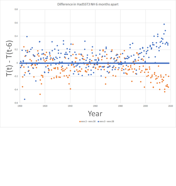
From the HadSST3 NH (or is it southern?)
http://woodfortrees.org/graph/hadsst3nh/from:1900
Its hard to see with the naked eye but 12 month smoothing and zooming in on the past 20 year highlights the problem. The plot below also highlights it.
I’ve plotted the difference in temperature anomalies 6 months apart. I also got the labels the wrong way around. The blue is for the months xxxx.5 and xxxx.58 minus xxxx.0 and xxxx.08, reespectively. The orange is for the other way around. You can see an oscillation starts to appear around 2000. Not completely random before but close and hardly likely to be natural. The modern data might be OK but with the data in the baseline period being rubbish so that you see a seasonal oscillation start to appear (these are differences from the mean for the month in the base period). These are over a half of the temperature increase since 1940.
We are basing policy on reconstructions, of CO2 levels as well as global temperatures, made from measurements not fit for purpose by people who get paid good money to make sure that they aren’t telling porkies. Even if unintentional, that they still have their jobs shows that there is a conspiracy.
Hi Hartmut, what an excellent post.
Although I did a very comprehensive research myself about uncertainties and error propagation in historical temperature data (land and sea) in order to prove or dismiss the claimed uncertainty of about ± 0.15 to ± 0,1 °C for the global mean, and by doing this checked most of the errors you mentioned also for SST, I am really surprised about the amount of new details about each error you fond out. Many thanks for that.
Just one point I want to add. Historical SST data are much more sparse than land temperature data, and spread over just a tiny fraction of the oceans due to commercial reasons, of course. In addition there mean is calculated in a complete different manner (I call this an algorithm) than land data. SST – as friendly John Kennedy told me, are summed of a given area for a complete month. And from this sum the average is taken. That means that one can´t really say what the mean SST for any year prior to the satellite era had been. At least not within an accuracy of ± 0,1 or • 0,15 °C. It must be some magnitudes higher. Regardless of the fact that the enormous heat inertia of water may allow less and more distant installed measuring points.
In contradiction to that land data per station are summed up by various algorithms over a day and than the daily average will be calculated. Solely the use of plenty of different algorithm by calculating the daily mean create overall an systematic error of min ± 0,23 °C. For those readers who are interested here is the paper about: https://www.eike-klima-energie.eu/wp-content/uploads/2016/07/E___E_algorithm_error_07-Limburg.pdf
Finally I want to add, that even random errors do not minimize to (near) zero as long there amount is big enough, but the lower limit is given by the hysteresis of the used instruments as Pat Frank (1) (2) showed in his excellent papers. In addition one have to take into account, as long as they are part of auto correlated time series – what they are- the minimum they can reach is about ± 0.4 °C as long the are taken for meteorological purpose. This was shown a while ago by some experts in statistics of Dresden Technical University, but unfortunately I was not able to dig it out in my collection of data.
For those readers who are able to read german my work is available here https://www.eike-klima-energie.eu/2016/04/03/analyse-zur-bewertung-und-fehlerabschaetzung-der-globalen-daten-fuer-temperatur-und-meeresspiegel-und-deren-bestimmungsprobleme/
An summary in english is available here https://www.eike-klima-energie.eu/wp-content/uploads/2016/07/Limburg_Summary__Dissertation_3-2.pdf
Best regards
Michael Limburg
m.limburg@eike-klima-energie.eu
P.S. Last but not least For the upcoming Porto Climate conference https://www.portoconference2018.org
I will attend and prepare a short introduction into this topic.
(1) P. Frank, “Uncertainty in the Global Average Surface Air Temperature Index: A
Representative Lower Limit,” Energy & Environment, vol. 21 , no. 8, pp. 969-989, 2010.
(2). P. Frank, “Imposed and Neglected Uncertainty in the Global Average Surface Air
Temperature Index,” Energy & Environment · , vol. Vol. 22, N, pp. 407-424, 2011.
For good measure I have checked the latest and best land temperature measurements.
NOAA has installed 104 new weather stations of the Climate Reference Network, partly in response to critique that older station surroundings unduly skew the accuracy of the data. The readings are logged and transmitted via satellite link.
The NOAA specification describes three redundant platinum resistance thermometers housed in fan aspirated solar radiation shields. An infrared temperature sensor is pointed at the ground surface to monitor unusual thermal radiation effects toward the thermometers.
The thermometer reads -60 to +300 deg C within ±0.04% accuracy over full range, and the 2003 Handbook for Manual Quality Monitoring describes inter-comparison of the three temperature sensors: Sensors should be within 0.3 deg C of one another.
The stated sensor error points to 0.04 % over 360 degree range, which is +/- 0.144 degrees. That value alone is five times greater than the desired accuracy of 0.03 degrees. Further, the flagging of a >0.3 degree differential between thermometers makes one question if a 0.29 (it being much greater than the specified 0.144 degrees) differential is deemed acceptable.
If they had more carefully selected the thermometer range, say from -60 to +60 degree C, with the same +/-0.04%, they could have inherently increased this accuracy three-fold to +/- 0.05 degrees!
Why would NOAA want to deprive itself of the ability to make SSTs whatever they want them to be by conducting such a reasonable experiment?
As HadCRU’s Phil Jones admitted, the corrupt book-cookers had to warm the ocean “data” to coincide with the bogus land “data”, so they did. Then along came NOAA’s Kar(me)lization of SST “data” in order to bust the “Pause”.
This is not science. It is the antithesis of science, as antiscientific as possible.