By Christopher Monckton of Brenchley
Skeptics 1, Fanatics 0. That’s the final score.
The corrected mid-range estimate of Charney sensitivity, which is equilibrium sensitivity to doubled CO2 in the air, is less than half of the official mid-range estimates that have prevailed in the past four decades. Transient sensitivity of 1.25 K and Charney sensitivity of 1.45 K are nothing like enough to worry about.
This third article answers some objections raised as a result of the first two pieces. Before I give some definitions, equations and values to provide clarity, let me make it plain that my approach is to accept – for the sake of argument only – that everything in official climatology is true except where we have discovered errors. By this acceptance solum ad argumentum, we minimize the scope for futile objections that avoid the main point, and we focus the discussion on the grave errors we have found.
Definitions
All definitions except that of temperature feedback are mainstream. I am including them in the hope of forestalling comments to the effect that there is no such thing as the greenhouse effect, or that temperatures (whether entire or delta) cannot induce feedbacks. If you are already well versed in climatology, as most readers here are, skip this section except for the definition of feedback, where climatology is at odds with mainstream feedback theory.
Greenhouse gases possess at least three atoms in their molecules and are thus capable of possessing or, under appropriate conditions, acquiring a dipole moment that causes them to oscillate in one of their vibrational modes and thus to emit heat.
Carbon dioxide (CO2), being symmetrical, does not possess a dipole moment, but acquires one in its bending vibrational mode on interacting with a near-infrared photon. To use Professor Essex’s excellent analogy, when a greenhouse gas meets a photon of the right wavelength it is turned on like a radiator, whereupon some warming must by definition occur.
The non-condensing greenhouse gases exclude water vapor.
Water vapor, the most significant greenhouse gas by quantity, is a condensing gas. All relevant changes in its atmospheric burden are treated as temperature feedbacks. Its atmospheric burden is thought to increase by 7% per Kelvin of warming in accordance with the Clausius-Clapeyron relation (Wentz 2007).
Emission temperature would obtain at the Earth’s surface if there were no non-condensing greenhouse gases or feedbacks present. Emission temperature is a function of insolation, albedo and emissivity (assumed to be unity), and of nothing else. As non-condensing greenhouse gases and feedbacks warm the atmosphere, the altitude at which the emission temperature obtains rises.
Radiative forcing (in W m–2) is an exogenous perturbation in the net (down minus up) radiative flux density at the top of the atmosphere. Forcings become warmings via –
The Planck sensitivity parameter (in K W–1 m2: Roe 2009), the quantity by which a radiative forcing is multiplied to yield the reference sensitivity. To a first approximation, it is the first derivative of the fundamental equation of radiative transfer with respect to the Earth’s emission temperature and emission flux density. Its value is thus dependent on insolation and albedo. The first derivative is the change in temperature per unit change in flux density, i.e., at today’s values 255.4 / (4 x 241.2) = 0.27 K W–1 m2. However, owing to altitudinal variation, the modeled value today is 0.31 = 3.2–1 K W–1 m2 (IPCC 2007, p. 631 fn.).
Temperature feedback (in W m–2 K–1), an additional forcing proportional to the temperature that induces it, in turn drives a feedback response (in K) that modifies the originating temperature. This definition of a feedback as a modification of a signal (not merely of a change in the input signal but also of the input signal itself) is standard in all applications of control theory except climatology, where it has been near-universally but falsely imagined that an input signal (emission temperature in the climate) does not induce a feedback, even where feedback processes are present and will modify even the tiniest change in that signal. It is this error that has misled official climatology into overestimating climate sensitivities.
Models do not implement feedback math explicitly. However, their outputs are routinely calibrated against past climate. Paper after paper incorrectly states that the entire 33 K difference between today’s surface temperature of 288 K and the emission temperature of 255 K that would prevail today in the absence of greenhouse gases or of feedbacks is driven by the directly-forced warming from the non-condensing greenhouse gases and the feedbacks induced by that warming.
For instance, Lacis (2010) says that three-quarters of the difference between emission temperature and today’s temperature is the feedback response to the non-condensing greenhouse gases: i.e, that the feedback fraction is 0.75, which, given the CMIP5 reference sensitivity of 1.1 K (Andrews 2012) would yield Charney sensitivity of 4.4 K. Sure enough, the CMIP5 models’ feedback fraction, at 0.67, is close to Lacis’ value, implying Charney sensitivity of 3.3 K. It will be proven that there is no justification whatever for mid-range estimates anything like this high. They arise solely because the models have been tuned over the decades to yield Charney sensitivities high enough to account for the entire 33 K.
- Reference sensitivity is the temperature change in response to a radiative forcing before taking feedbacks into account.
- Equilibrium sensitivity, the warming expected to occur within a policy-relevant timeframe once the climate has resettled to equilibrium after perturbation by a radiative forcing (such as doubled CO2 concentration) and after all temperature feedbacks of sub-decadal duration have aced, may be somewhat larger than –
- Transient climate sensitivity, the warming expected to occur immediately in response to a forcing. The chief reason for the difference is the delay occasioned by the vast heat-sink that is the ocean.
- Charney sensitivity, named after Dr Jule Charney, is equilibrium sensitivity to doubled CO2.
Zero-dimensional-model equation relates reference and equilibrium sensitivities or temperatures via the feedback fraction, which accounts for the entire difference between them. Control theory in all applications except climatology uses both forms of (1) and of its rearrangement, (2), but climatology has not hitherto appreciated that the right-hand form of each equation is permissible. For this reason, it has failed to accord sufficient – or in most instances any – weight to the feedback response that arises from the presence of emission temperature. As a result of this grave error, official climatology has greatly overestimated the feedback fraction and hence all transient and equilibrium climate sensitivities.
![]()
Input variables
Input variables are from official sources. Net industrial-era anthropogenic radiative forcing to 2011 was 2.29 W m–2 (IPCC 2013, table SPM.5); the Planck sensitivity parameter is 3.2–2 K W–1 m2 (IPCC 2007, p. 631 fn.); the radiative energy imbalance to 2010 was 0.59 W m–2 (Smith 2015); industrial-era warming to 2011 was 0.75 K (least-squares trend on the HadCRUT4 monthly global mean surface temperature anomalies, 1850-2011: Morice 2012); and the radiative forcing at CO2 doubling is 3.5 W m–2 (Andrews 2012); the Stefan-Boltzmann constant is 5.6704 x 10⁻⁸ W m–2 K–4 (Rybicki 1979); albedo without non-condensing greenhouse gases or feedbacks would be 0.418 (Lacis 2010); global mean surface temperature without greenhouse gases would be 252 K (ibid.); and today’s global mean surface temperature is 288.4 K (ISCCP 2016).
Mid-range industrial-era Charney sensitivity
Now for the simplest proof of small Charney sensitivity. Net industrial-era manmade forcing to 2011 was 2.29 W m–2, implying industrial-era reference warming 2.29 / 3.2 = 0.72 K. The radiative imbalance to 2010 was 0.59 W m–2. Warming has thus radiated 2.29 – 0.59 = 1.70 W m–2 (74.2%) to space. Equilibrium warming to 2011 may thus prove to have been 34.7% greater than the observed 0.75 K industrial-era warming to 2011. The feedback fraction for transient sensitivity is then f = 1 – 0.716 / 0.751 = 0.047, so that transient climate sensitivity is 1.09 / (1 – 0.047) = 1.15 K. Industrial-era f for equilibrium sensitivity is 1 – 0.716 / (0.751 x 1.347) = 0.29, implying Charney sensitivity 1.09 / (1 – 0.29) = 1.55 K.
That’s it. Charney sensitivity is less than half of the 3.3 K mid-range estimate in the CMIP3 and CMIP5 general-circulation models, distorted as they are by the long-standing misallocation of all 33 K of the difference between today’s temperature and emission temperature to greenhouse-gas forcings and consequent feedbacks.
Mid-range pre-industrial Charney sensitivity
To show how official climatology’s grave error arose, we shall study how it has been apportioning that 33 K difference between today’s temperature and emission temperature.
Lacis (2010) estimated albedo without greenhouse gases as 0.418, implying emission temperature [1364.625(1 – 0.418) / (4σ)]0.25 = 243.26 K (Stefan-Boltzmann equation, with unit emissivity). However, Lacis estimated the global mean surface temperature without non-condensing greenhouse gases as 252 K, implying a small feedback response to emission temperature, arising from melting equatorial ice and about 10% of the current atmospheric burden of water vapor. That 10% value can be obtained from the 7% per Kelvin increase in water vapor found in Wentz (2007): thus, 100 / 1.0733 = 10.7.
Global temperature in 1850 was 287.6 K. The 35.6 K difference between 287.6 and 252 K was given as 25% [8.9 K] directly-forced warming from the naturally-occurring, non-condensing greenhouse gases and 75% [26.7 K] feedback response to that greenhouse warming. However, if the feedback fraction f over Lacis’ 50-year study period were constant, for transient sensitivity f would be 1 – (243.26 + 8.9) / 287.6 = 0.123, and transient sensitivity itself would be 1.09 / (1 – 0.123) = 1.25 K. If an energy imbalance in 1850 might eventually increase that year’s temperature by 10%, then f = 1 – (243.26 + 8.9) / (287.6 x 1.1) = 0.203. Charney sensitivity would then be 1.09 / (1 – 0.203) = 1.4 K.
In Lacis, the 44.2 K difference between emission and 1850 temperatures comprises 8.7 K (3.6%) feedback response to the 243.3 K emission temperature and, since Lacis takes transient-sensitivity f = 0.75, directly-forced greenhouse warming of 8.9 K inducing 26.6 K (300%) feedback response. Thus, Lacis imagines the feedback responses to emission temperature and to direct greenhouse warming are 3.6% and 300% respectively of the underlying quantities, which is absurd. What is more, Lacis says that the feedback fraction 0.75 applies also to “current climate”, an explicit demonstration that climatology’s error leading to overstatements of equilibrium sensitivity in the models arose from its neglect of the large feedback response to emission temperature.
Our corrected method finds transient-sensitivity f a lot less that Lacis’ 0.75. It is just 0.123. Then the 44.2 K difference between 1850 temperature and emission temperature comprises 243.3 f / (1 – f) = 34.1 K feedback response to emission temperature; 8.9 K directly-forced greenhouse warming; and 8.9 f / (1 – f) = 1.2 K feedback response to direct greenhouse warming. Thus, feedback responses to emission temperature and direct greenhouse warming are identical at f / (1 – f) = 14% of the underlying quantities.
In practice, ice-melt would steadily reduce the ice-covered surface area, reducing the surface-albedo feedback and hence the overall feedback fraction, though that effect might be largely canceled by increased water vapor and cloud feedback. The assumption of a uniform feedback fraction throughout the transition from emission temperature to 1850 temperature is, therefore, not unreasonable. Other apportionments might be made: but it would not be reasonable to make apportionments anywhere close to those of Lacis or of the CMIP models.
Note how well the industrial and pre-industrial sensitivities cohere, and how very much smaller they are than official climatology’s 0.67-075. The corrected industrial-era values, just 1.25 K transient sensitivity and 1.55 K equilibrium sensitivity, necessarily follow from the stated official definitions and values. In my submission, it is no longer legitimate for official climatology to maintain that the mid-range estimate of Charney sensitivity is anything like as high as the CMIP3/CMIP5 models’ 3.3 K.
Certainty about uncertainties
What of the uncertainties in our result? Some of the official input values on which we have relied are subject to quite wide error margins. However, because our mid-range estimate of Charney sensitivity is low, occurring at the left-hand end of the rectangular-hyperbolic curve of Charney sensitivities in response to various values of the feedback fraction, the interval of plausible sensitivities is nothing like as broad as the official interval, which I shall now demonstrate to be a hilarious fiction.

The Charney report of 1979, echoed by several IPCC Assessment Reports, gives a Charney-sensitivity interval 3.0 [1.5, 4.5] K. The 2013 Fifth Assessment Report retains the bounds but no longer dares to state the mid-range estimate, for a reason that I shall now reveal.
By now it will be apparent to all that the chief uncertainty in deriving transient or equilibrium sensitivities is the value of the feedback fraction. I found it curious, therefore, that IPCC did not derive its mid-range estimate of Charney sensitivity from the mean of the bounds of the feedback fraction’s interval. The mismatch is quite striking (see below)
IPCC’s mid-range Charney sensitivity 3.0 K implies a feedback fraction 0.61, which is three times closer to the upper bound 0.74 than to the lower bound 0.23. If IPCC had derived its mid-range Charney sensitivity from a value of the feedback fraction midway between the bounds, its 3 K mid-range estimate would have fallen by an impressive 0.75 K to just 2.25 K:

How, then, did IPCC come to imagine that mid-range Charney sensitivity could be as high as 3 K? The Charney Report of 1979, the first official attempt to derive Charney sensitivity, provides a clue. On p. 9, Charney found that the interval was 2.4 [1.6, 4.5] K, implying a feedback fraction close enough to the mean of its bounds. However, by p. 16 he had decided that his eponymous interval was “in the range 1.5-4.5 K, with the most probable value near 3 K”. Why did he go for 3 K? And why did IPCC and CMIP5 remain in that ballpark for four decades? Perhaps it was because, owing to their error, they could not otherwise account for the 33 K difference between emission temperature and present-day temperature.

Be that as it may, where (a) the feedback fraction is defined as 1 minus the ratio of reference to equilibrium temperature (Eq. (2)), where (b) the mid-range value of the feedback fraction is the mean of the bounds of its interval, and where (c) the mid-range estimate of equilibrium sensitivity is twice the lower-bound estimate, the upper bound of the feedback fraction must be unity. Then the upper bound of equilibrium sensitivity will fall precisely on the singularity in the rectangular-hyperbolic response curve, and will therefore be somewhere between plus and minus infinity (see above). This is definitive evidence that the supposed Charney-sensitivity interval 3.0 [1.5, 4.5] K is nonsense, and that all attempts to ascribe a statistical confidence interval to it are likewise nonsense.
Is our mid-range estimate of Charney sensitivity reasonable?
Rud Istvan, in one of many interesting comments on the earlier articles, says Lewis & Curry (2014) found transient and equilibrium sensitivities to be 1.3 K and 1.65 K respectively, implying that Charney sensitivity is 1.25 times transient sensitivity, not 1.37 times as I calculated earlier. In that event, the feedback fraction is 1 – 0.716 / (0.751 x 1.25) = 0.237, implying Charney sensitivity 1.09 / (1 – 0.237) = 1.45 K, similar to the 1.5 K in Lewis 2015.
Rud offers the following interesting confirmatory method. In IPCC (2013), the mid-range estimates of the sub-decadal temperature feedback sum is 1.6 W m–2 K–1, since the feedbacks other than the water-vapor feedback sum to zero. Multiplying the feedback sum by the Planck parameter gives a mid-range feedback fraction 0.5 (Table 1). Note in passing that, as discussed earlier, the upper-bound feedback fraction works out at the absurd value 1.0.

Rud goes on to point out that, as several papers show, the CMIP5 models produce about half the observed rainfall, implying that the modeled water-vapor feedback is double the true value. Therefore, he says, the true feedback fraction is half the CMIP5 models’ estimate. That means 0.25, giving a Charney sensitivity of 1.09 / (1 – 0.25) = 1.45 K.
I shall let Rud Istvan have the last word:
“This is not coincidental. The ‘best’ Charney sensitivity, whether calculated using the energy budget, or observed v. modeled via Bode’s feedback fraction f, is half of the ‘best estimate’ in IPCC (2007). I agree with Christopher Monckton of Brenchley. It’s game over.”
Why are people talking about such low radiation numbers as 240 W/m^2 on this site?
https://www.smhi.se/en/climate/climate-indicators/climate-indicators-global-radiation-1.91484
http://www.inforse.org/europe/dieret/Solar/asolarirrad.gif
Somebody has some explaining to do!
“Somebody has some explaining to do!”
I think you need to look at units. They are in kWh/m2/year.
Yeah, I know. However,
240*24=5.76kWh/m^2
On the map, that is tropical, not -18C territory.
Can you explain this to me?
Zoe Phin April 2, 2018 at 7:30 pm
Why are people talking about such low radiation numbers as 240 W/m^2 on this site?
Because that’s what it is?
Somebody has some explaining to do!
Indeed you do! Can’t you read a graph?
240*24=5.76kWh/m^2. According to the map, that’s tropical climate!
It also shows rainforests cooler than deserts (year round, day and night averaged), so so much for bunk GHG-warming theory!
“240*24=5.76kWh/m^2. According to the map, that’s tropical climate!”
And you were saying that 240 is too low! Explaining needed.
But the 240W/m2 is the total sunlight that is thermalised, and subsequently emitted as IR. It is not the amount reaching the surface. According to the Trenberth budget, 161 W/m2 reached the surface. 78 W/m2 is absorbed in the atmosphere, but is still added to the climate system.
Nick,
161*24=3.9kWh/m^2
The map shows that to be mediterranean climate.
However
240 = -18C
161 = -42C
Your answer didn’t help. Please try again .
Zoe Phin April 2, 2018 at 8:02 pm
240*24=5.76kWh/m^2. According to the map, that’s tropical climate!
You don’t appear to know how to calculate kWh!
Phil, then why don’t you impress us all and show us how it’s done.
Lord Monckton writes: “Zero-dimensional-model equation relates reference and equilibrium sensitivities or temperatures via the feedback fraction, which accounts for the entire difference between them. Control theory in all applications except climatology uses both forms of (1) and of its rearrangement, (2), but climatology has not hitherto appreciated that the right-hand form of each equation is permissible.”
Our climate isn’t governed by control theory or the mathematics of amplifiers. Our climate is governed by the laws of physics in general and radiation in particular. Under limited circumstances (temperature changes of a few degK), one might say that equation 1 has some validity:
eqn 1: dT = dT_0 / (1-f)
However, the reality that temperature depends on RADIATION has been edited out of equation 1. The reality that emission of radiation depends in a non-linear manner on temperature has also been lost. W = eoT^4. Non-linearity means that Monckton’s conclusions are incorrect.
Nothing in the physics of climate produces the right-hand version of Monckton’s equations. Feedback is a phenomena associated with temperature CHANGE, not with temperature itself.
If Frank considers that climate is not governed by feedback processes, then global warming will not exceed 1.1 K per CO2 doubling. If he considers, in line with official climatology, that feedback processes do subsist in the climate, then those processes are subject to the same mathematics as feedback processes in any dynamical system. If Frank now disagrees with this, as no doubt he wishes to, then he should address his complaint to official climatology and not to me. IPCC (2013), for instance, mentions “feedback” >1100 times. Let him address his opinions to secretariat@ipcc.ch.
Frank appears to imagine that feedback mathematics applies only where the perturbations of the input signal are small. However, there is no warrant for any such novelty in the literature in which the mathematics of feedback is expounded. Of course, if Frank were correct on this point, then it would certainly not be possible for feedback processes to increase the direct warming driven by greenhouse gases by even a factor 2, let alone an order of magnitude, as some extremist authorities have misguidedly tried to suggest.
Frank then makes the error – common among non-physicists – of assuming that the mathematics of feedback cannot apply to the climate because temperature is dependent upon radiation, which does not feature in the zero-dimensional-model equation.Frank should address his concerns to official climatology, not to me. He here perpetrates three further errors: first, he imagines that the linear zero-dimensional-model equation cannot be adapted to handle nonlinearities in feedback processes, which is not the case (see e.g., Roe 2009). Secondly, he imagines, on no stated evidence, that in the climate the feedback processes are sufficiently nonlinear to justify abandoning the zero-dimensional-model equation in the form in which climatology has used it for at least half a century. Thirdly, he imagines that because the fundamental equation of radiative transfer is a fourth-power relation its first derivative (which, of course, is what we are concerned with when talking of changes in radiation) must be nonlinear. Here, a little elementary calculus will demonstrate the falsity of that proposition. Under official climatology’s harmless assumption that emissivity is constant at unity, the first derivative of the Stefan-Boltzmann equation, expressed in terms of temperature T and radiative flux density Q, is simply T / (4Q), which is self-evidently linear.
Next, Frank states that “Nothing in the physics of climate produces the right-hand version of Monckton’s equations”. As I have suggested before, Frank should read ch. 1 of Bode (1945), taken with the definitions of the input and output signals E0, ER respectively on p. vii. He should then read the numerous papers in the reviewed literature which cite Bode as their authority for feedback mathematics in the climate. He will see that those sources have misunderstood the elementary physics of feedback, in that their cut-down and degenerate version of the zero-dimensional-model equation given in Bode makes no allowance for the input signal and none, therefore, for the substantial feedback response thereto, which they mistakenly add to the actually very small feedback response to the presence of the naturally-occurring, non-condensing greenhouse gases.
Finally, Frank says that “Feedback is a phenomena” [one imagines he means “pheonomenon”] associated with temperature change, not with temperature itself.” That, indeed, is a fairish statement of official climatology’s error. It is remarkably simple to demonstrate that climatology’s error is indeed an error. All one needs to do is to take the input temperature of 255 K (which, as far as feedback processes are concerned, is a temperature change of 255 K compared with no temperature at all), and divide it by (1 – 0.08), where 0.08 is the feedback fraction derived in the first of our three articles. Note that we have not made any amplification in the 255 K before subjecting it to feedback. Is the output signal 255 K? Of course it isn’t. It’s 277 K. Where, then, did the additional 22 K come from, if not from the feedback response to emission temperature itself?
Frank, like others here, may assume that he is dealing only with an autodidact Claccisist. However, one of my co-authors is a professor of applied control theory. If climatology wishes to pray feedback mathematics in aid at all, then it must learn to follow the correct mathematics, or it will lead itself into errors such as its present large error. Remove that large error and all concern about excessive warming of the climate vanishes. There will still be some warming, but nothing like enough to worry about.
“Where, then, did the additional 22 K come from, if not from the feedback response to emission temperature itself?”
Temperature can be increased by two means: Heat and Work. You forgot Work done on [all] atmospheric gases.
What work?
The gravitational work on all atmospheric gases.
Bode talks about additive quantities, ike current.
Monckton talks about non-additive quantity: temperature.
I just don’t see electronic signal feedback theory as appropriate for climate domain.
I don’t see amplifiers gaining free energy beyond what the wall plug provides.
But it’s claimed that gases can amp up their temperature (beyond what the sun provides) just because they have a temperature.
Temperature is an effect of forces, a measure really, not a force unto itself. It can’t do anything, it takes what its given. Only forces can increase temperature.
Like I told you
The atmosphere has too little mass to control global T. CO2 warming does not exist. It is a red herring. It is beyond me who even thought of it first.
It is really the oceans that catch and transport heat.
The UV that gets absorbed eventually changes to simple heat. What varies UV? You tell me.
The water vapor in the atm does.
Lord Monckton wrote: “If Frank considers that climate is not governed by feedback processes, then global warming will not exceed 1.1 K per CO2 doubling. If he considers, in line with official climatology, that feedback processes do subsist in the climate, then those processes are subject to the same mathematics as feedback processes in any dynamical system. If Frank now disagrees with this, as no doubt he wishes to, then he should address his complaint to official climatology and not to me. IPCC (2013), for instance, mentions “feedback” >1100 times. Let him address his opinions to secretariat@ipcc.ch”
Frank believes that our climate is governed by the laws of physics in general and the laws of radiation in particular. Mathematics that government LINEAR amplifiers and LINEAR control systems do not apply to apply to our climate system in general.
It is perfectly possible to describe our climate system without using amplification:
dW(T)/dT = -λ(T) dW = λ*dT and dT = dW/λ and dW/dT = λ
where W(T) is the net flux of radiation across the TOA expressed as a function of the surface temperature (T, sometimes written as Ts). λ(T) is the derivative of W(T) with respect to T and is called the climate feedback parameter. It is NOT a constant.
In general, emission of radiation varies with T^4, meaning that λ(T) varies with T^3. This is called Planck feedback. For example, if we assume a gray body model for emission of radiation: W(T) = -eoT^4, then λ(T) = -4eoT^3. If we adapt this model to the Earth (T = 288, e = 0.615), then: λ(T=288) = -3.332 W/m2/K, λ(T=289) = -3.3367 W/m2/K, λ(T=291) = -3.437 W/m2/K and λ(T=293) = -3.508 W/m2/K. After 5K of global warming, assuming λ(T) is a constant involves making a 5% error (in a gray body model). An error this size may or may not be tolerable. When considering a planet 33K cooler, λ(T=255) = -2.313 W/m2/K. Assuming λ(T) is constant over this temperature range makes a 30-40% error. This is an enormous error and explains why Monckton’s results are so different from those produced by others, AND WRONG.
The Earth isn’t a simple gray body. AOGCMs uses more sophisticated physics to determine λ(T) for the planet. Climate scientists using AOGCMs and a narrow range of temperature (1K or a few K) and no other feedbacks to calculate a special value for dW/dT called λ0 = -3.2 W/m2/K. However, that more sophisticated physics relies on the Planck function, B(λ.T) and therefore produces thermal radiation that varies roughly with T^4. If AOGCMs were used to calculate a λ0 for work near 255K, the result would be a much smaller value than -3.2 W/m2/K.
Thermal emission of radiation (Planck feedback) isn’t the only thing that changes the net flux across the TOA when the surface of the planet warms, so ECS involves more than just λ0. However, once one has made a serious error in λ0, everything else one does is hopelessly wrong.
Monckton is applying mathematics for linear feedback to the Earth, where it is trivial to prove that feedback is not linear over the temperature range used 255 K to 288 K. To get the correct answer, Monckton needs to start with the physics of radiation, not the mathematics of amplifiers, control theory. That mathematics is only appropriate for small changes in temperature where λ can be treated as if it were constant.
Frank, a rhetorical question not addressed to you.
Why do people always assume an imbalance if there even is one(which I highly doubt even if the satellites had the required accuracy), applies across the entire BB spectrum?
It wouldn’t, it can’t. Even if all the co2 spectrum was blocked, which it isn’t either, the optical window isn’t.
It’s like being worried you’re going to over fill your bucket while half the bottom is gone.
Monckton writes: “Frank then makes the error – common among non-physicists – of assuming that the mathematics of feedback cannot apply to the climate because temperature is dependent upon radiation, which does not feature in the zero-dimensional-model equation.Frank should address his concerns to official climatology, not to me.
The IPCC does not use a [linear] zero-dimensional model for any serious climate studies.
Monckton continues: “He here perpetrates three further errors: first, he imagines that the linear zero-dimensional-model equation cannot be adapted to handle nonlinearities in feedback processes, which is not the case (see e.g., Roe 2009).”
Roe (2009) does indeed mention that the zero dimensional model can be modified when necessary to handle non-linearity. See p102. http://earthweb.ess.washington.edu/roe/Publications/Roe_FeedbacksRev_08.pdf Applying Equation 32 to a graybody model for emission with T=255K, ΔT=33K, e=0.615
-ΔW = (dW/dT)*ΔT + 0.5*(d2W/dT2)*(ΔT)^2 + smaller terms
-ΔW = (4eoT^3)*ΔT + 0.5*(12eoT^2)*(ΔT)^2
-ΔW = {(4eoT^3) + 0.5*(12eoT^2)*(ΔT)}*ΔT
-ΔW = {2.313 + 0.449}*ΔT = 2.762*ΔT
λ = -2.762 not -3.332 W/m2/K from a purely linear model
In other words, Roe (2009) says that Monckton is WRONG and that serious corrections are needed for non-linearity. And the first two terms from Roe’s correction for non-linearity aren’t adequate since the correct values for λ is -3.33 W/m2/K. If the factor of 0.5 is omitted in equation 32, λ with the second order correction becomes a much more reasonable -3.21 W/m2/K.
Finally Monckton says: “[Frank] imagines, on no stated evidence, that in the climate the feedback processes are sufficiently nonlinear to justify abandoning the zero-dimensional-model equation in the form in which climatology has used it for at least half a century.”
Frank has PROVEN that the simplest feedback process (Planck feedback) is sufficiently non-linear to invalidate Monckton’s results. Everyone else immediately recognizes the problem, so no climate scientist has ecer applied Monckton’s equations to a 33 degK change in temperature.
Finally Monckton writes: “Frank, like others here, may assume that he is dealing only with an autodidact Claccisist. However, one of my co-authors is a professor of applied control theory. If climatology wishes to pray feedback mathematics in aid at all, then it must learn to follow the correct mathematics, or it will lead itself into errors such as its present large error.
You don’t need a professor of control theory, because the equations of linear control theory don’t apply to this particular PHYSICS problem. There are plenty of skeptical physics and climate science professors who would be thrilled to endorse your physics, if it were correct.
If anyone is still interested, the problems with Monckton’s application of control theory go far deeper than just the serious non-linearity of emission of thermal radiation over 255 to 288 K. That non-linearity means that λ0 can not be treated as a constant. However, as shown below, the feedback factor f is also not a constant. Monckton ignores the physics that creates f, so he doesn’t realize it can’t be treated as a constant.
ΔT = -ΔW/λ
This is the standard way to calculate warming from a forcing ΔW. One doesn’t need to get involved with amplification at all. So where does amplification come from? We break the climate feedback parameter into components:
λ = λ_0 + λ_WV + λ_LR + λ_cloud + λ_surface albedo = λ0 + λ1
where these terms are Planck, WV, LR, cloud, and surface albedo feedbacks. The IPCC does this to understand what phenomena besides thermal radiation change with the surface of the planet warms. Decomposing λ in this manner isn’t necessary and the AOGCMs that do so are currently incapable of accurately reproducing the phenomena that create these feedbacks. Lord Monckton doesn’t accept these values because they say climate sensitivity is 2.2 to 4.7 K/doubling. For purposes of understanding amplification, only Planck feedback, λ0, and the sum of all other feedbacks, λ1,are needed. The other feedbacks are involve highly non-linear phenomena, so λ1 is not a constant.
ΔT = -ΔW/(λ0 + λ1) = -(ΔW/λ0)/(1+ λ1/λ0) = (ΔT_0)/(1-f)
-(ΔW/λ0) is the no-feedbacks climate sensitivity ΔT_0 since it arises only from Planck feedback. f = -λ1/λ0. So -f is the ratio of two parameters λ0 and λ1 that vary with temperature. Climate scientists only these equations for small changes in temperature (a few degK) and they are concerned about non-linearity when they do. It is totally absurd to act as if f and λ0 are constants from 255K to 288K.
We can think of climate change as a stepwise process:
1) A doubling of CO2 creating a ΔT_0 rise in temperature.
2) A ΔT_0 rise in temperature creating an additional f*ΔT_0 rise in temperature due to feedbacks.
3) That f*ΔT_0 rise in temperature creating an additional f^2*ΔT_0 rise in temperature due to feedbacks.
4) 3) That f^2*ΔT_0 rise in temperature creating an additional f^3*ΔT_0 rise in temperature due to feedbacks.
5) And so on.
Summing the infinite series gives:
ΔT = ΔT_0 * ( 1 + f + f^2 + f^3 + …)
ΔT = ΔT_0 / (1-f)
So we can mathematically describe forced warming in terms of a single climate feedback parameter λ characteristic of our planet of our planet or a combination of Planck feedback and other feedbacks. One set of equations makes it appear as if no-feedbacks warming is being amplified. The second, simpler equation does not. Amplification is an unnecessary complication that arises from feedbacks that are not linear over more than a few degK and the non-linearity is a far more severe problem. From a pragmatic perspective, λ around -1 W/m2/K means climate sensitivity is around 3.7 K/doubling. λ around -2 or lower means EBMs are correct and climate sensitivity is below 2 K/doubling. But don’t expect either answer to be remain valid over a wide range of temperature.
micro6500 April 3, 2018 at 8:00 pm asked: Why do people always assume an imbalance if there even is one(which I highly doubt even if the satellites had the required accuracy), applies across the entire BB spectrum? It wouldn’t, it can’t. Even if all the co2 spectrum was blocked, which it isn’t either, the optical window isn’t. It’s like being worried you’re going to over fill your bucket while half the bottom is gone.
We care about a radiative imbalance because anytime an object gains more energy than it loses (through all means including work), the law of conservation of energy says that the imbalance becomes internal energy/higher temperature. Heat capacity is the factor that converts that energy (technically power) into a higher temperature (technically a rate of warming that persists as long as the imbalance exists). We are concerned about the radiative imbalance summed over ALL wavelengths, because that is the only way heat enters and leaves the planet. Using that first approximation, we know somewhere below the TOA heat is accumulating, but we can’t say where. (Where is why we need climate models – to handle convection transfer of latent and simple heat WITHIN the climate system).
Due to the fact that there is negligible overlap between the wavelengths used by incoming SWR and outgoing LWR, different things can interfere differentially with one process or another. A GHG might be defined as a gas that interferes with outgoing OLR more than incoming SWR. Clouds and surface snow/ice reflect SWR and absorb LWR.
If this happens, the warmer molecules dump energy into molecules by conduction if required that can cool out the optical window, the wavelengths are just shifted. Line emitters can be blocked in this fashion, and they might get warmer, but then it’s conducted into a BB emitter where it’s radiated that way.
It’s not accumulating, why I’ve shown that chart 1,000 times. WV defines min surface temp, and any excess warming from co2 is radiated prior to wv slowing the cooling rate, other wise air temps don’t drop initiating the wv feedback that slows cooling.
Micro6500 wrote: If this happens, the warmer molecules dump energy into molecules by conduction if required that can cool out the optical window, the wavelengths are just shifted. Line emitters can be blocked in this fashion, and they might get warmer, but then it’s conducted into a BB emitter where it’s radiated that way.
Franks adds: It is possible you are referring to “local thermodynamic equilibrium” or LTE. See Grant Petty’s book for example. LTE means that molecules exchange energy by collisions much faster than by any other process – which means there is a thermodynamics temperature for a group of molecules that depends only on their mean kinetic energy. The fraction of molecules in any excited state – and therefore their emission rate – depends only on the local temperature, and not excitation on by the local radiation field. The troposphere and lower stratosphere are in LTE.
LTE doesn’t imply simple “thermodynamic equilibrium” between radiation and the medium/molecules through which the radiation is passing. Planck’s Law describes radiation in equilibrium with matter. When such equilibrium exists radiation at all wavelengths has blackbody intensity given by Planck’s Law. This doesn’t happen at all wavelengths in our atmosphere. SWR passes right through. So does LWR in the atmosphere in the atmospheric window.
Frank wrote: Using that first approximation [imbalance across the TOA], we know somewhere below the TOA heat is accumulating, but we can’t say where.
Micro6550 replied: It’s not accumulating, why I’ve shown that chart 1,000 times. WV defines min surface temp, and any excess warming from co2 is radiated prior to wv slowing the cooling rate, other wise air temps don’t drop initiating the wv feedback that slows cooling.
Frank replies: As best I can tell, in this one locations for a few days, the fall in temperature late at night is limited by condensation of water vapor. Any model that doesn’t reproduce this will be too cold for a few hours at night under these conditions and therefore radiatively cool less than it should. However, any error is minor. GHGs near the surface of the Earth are very ineffective at moving heat further away from the surface, because they radiate most often at wavelengths they absorb most strongly. When the average photon travels only a 100 meters before being absorbed, the flux of upward and downward LWR doesn’t produce a net upward flux of heat. The temperature gradient near the surface is mostly controlled by turbulent mixing and/or convection and rarely by radiation.
At night, unless weather fronts are moving through, it’s almost always calm. Ie cooling is almost all radiative. And it matters enough that the correlation between Tmin and dew point is 97%, and 96% between Tmax and dew point.
Frank continues to miss – or perhaps deliberately to divert attention away from – the main point of this series, which is that if proper allowance is made for the large feedback response to emission temperature then – whether the feedback regime be linear or nonlinear – the feedback fraction must be considerably smaller than where less than proper allowance is made.
Though Frank – like others here – expatiates on nonlinearity, relying on a reference that I had supplied to him, he provides no evidence that the net nonlinearity causes equilibrium sensitivity to rise with temperature.
As to the Planck “feedback”, which – as Roe (2009) points out – is best understood not as a feedback at all but as part of the reference system, Frank has already had it explained to him that our derivation of the feedback fraction depends upon the Planck parameter only insofar as it relates to the narrow interval of some 2-3 K between the temperature in 1850 and the temperature at doubled CO2 concentration compared with today. The influence of the nonlinearity in that parameter is, therefore, minuscule as far as our calculation is concerned.
Frank appears not to know that control theory is a branch of physics, and that it is of universal application in all dynamical systems – such as climate – upon which feedbacks bear.
Frank also incorrectly assumes that the interval over which nonlinearity in feedbacks operates is 255-288 K. No: once due allowance is made for the feedback response to emission temperature, the interval is more like 277-287 K. The Planck parameter at 277 K is 277 / 4 / 241.2 = 0.29 Kelvin per Watts per square meter. At 287 K it is 287 / 4 / 241.2 = 0.30 Kelvin per Watt per square meter. Indeed, even if we go down to 255 K, it falls only to 255 / 4 / 241.2 = 0.26 Kelvin per Watt per square meter (in each instance, I use the Schlesinger ratio to derive the Planck parameter).
Frank asserts, on no evidence, that “Monckton ignores the physics that creates the feedback fraction, so he doesn’t realize it can’t be treated as a constant.” That assertion is culpably false, given that I had expressly discussed the question of nonlinearity in the series of head postings.
The central point is that, however nonlinear the system is (and Frank’s favorite example, the Planck parameter, turns out to be nothing like as nonlinear as he had hoped we might believe), if the feedback response to emission temperature is taken properly into account the feedback fraction will be less than if it is not taken properly into account.
If Frank considers that there is a strong nonlinearity in the feedback fraction depending upon the Earth’s surface temperature, then where does that strong nonlinearity come from? It certainly does not come from the Planck parameter. Nor does it come from the feedback response to the water vapor and lapse-rate feedbacks. So, where does it come from?
Of course it comes from water vapor, and if you look at the difference between daytime lapse rate and nighttime lapse rate, it is that loss of energy that maintains temps during the night (since it is radiated in all directions) as water vapor is converted to liquid, but in the same process a lot of that IR goes right back into evaporating those same molecules, the residual that’s left is dew.
But it also has a negative response to increasing noncondensing ghg’s, because of the relationship between the vapor pressure of water, pressure and air temps.
This data shows the 35W/m^2 feedback response from the process on surface temps.
Monckton of Brenchley April 3, 2018 at 3:33 am
Thirdly, he imagines that because the fundamental equation of radiative transfer is a fourth-power relation its first derivative (which, of course, is what we are concerned with when talking of changes in radiation) must be nonlinear. Here, a little elementary calculus will demonstrate the falsity of that proposition. Under official climatology’s harmless assumption that emissivity is constant at unity, the first derivative of the Stefan-Boltzmann equation, expressed in terms of temperature T and radiative flux density Q, is simply T / (4Q), which is self-evidently linear.
Well if emissivity is assumed to be unity then the S-B equation is:
Q=σT^4
The first derivative of which is:
dQ/dT=4σT^3
So I’m not sure where Monckton gets his expression from but the first derivative is ‘self-evidently’ nonlinear. Perhaps he has performed a series expansion?
” the first derivative of the Stefan-Boltzmann equation, expressed in terms of temperature T and radiative flux density Q, is simply T / (4Q), which is self-evidently linear.”
It’s actually (4Q)/T. Neither expression is linear in T, since Q depends on T.
Monckton replies: Though Frank – like others here – expatiates on nonlinearity, relying on a reference that I had supplied to him, he provides no evidence that the net nonlinearity causes equilibrium sensitivity to rise with temperature.
As to the Planck “feedback”, which – as Roe (2009) points out – is best understood not as a feedback at all but as part of the reference system, Frank has already had it explained to him that our derivation of the feedback fraction depends upon the Planck parameter only insofar as it relates to the narrow interval of some 2-3 K between the temperature in 1850 and the temperature at doubled CO2 concentration compared with today. The influence of the nonlinearity in that parameter is, therefore, minuscule as far as our calculation is concerned.”
Frank replies: I didn’t need Roe to know about non-linearity. YOU claimed that Roe said non-linearity could be tolerated. Since you didn’t apply the equations Roe recommended for non-linearity, I was able show that you made a serious error. Either apply the CORRECT EQUATIONS from Roe or admit that your answer is WRONG because you haven’t done so!
Non-linearity is only a proven problem for large changes in temperature, such as calculations using dT = 33K. For small changes (dT = about 1 K) there is a second problem: Current warming is a transient, not an equilibrium, response to current forcing. Current ocean heat uptake is about 0.7 W/m2 while current forcing is about 2.5 W/m2, which means that current warming is about 70% of the way to equilibrium warming, a non-trivial error. The correct way to deal with that situation is with energy balance models. See: Lewis and Curry (2015) with a central estimate of ECS of 1.6 K (f = 0.28), but a wide 95% confidence interval ranging from 1 to 4 K. Otto et al found about 2 K (f = 0.42). f = 0.08 is grossly wrong.
Monckton: Frank appears not to know that control theory is a branch of physics, and that it is of universal application in all dynamical systems – such as climate – upon which feedbacks bear.
Frank knows that control theory is a branch of engineering, ie applied physics! You must start with the correct physics that APPLIES to the engineering problem you are trying to address. Simplifying the physics of climate to a simple linear model (which Roe says needs modification for non-linearity) and applying that model to a world without condensable GHGs is absurd. So is ignoring the difference between transient and equilibrium warming.
Monckton writes: If Frank considers that there is a strong nonlinearity in the feedback fraction depending upon the Earth’s surface temperature, then where does that strong nonlinearity come from? It certainly does not come from the Planck parameter. Nor does it come from the feedback response to the water vapor and lapse-rate feedbacks. So, where does it come from?
Frank replies: What nonsense! As I mentioned earlier, using a simple gray body model, Planck feedback λ0 = dW/dT = 4eoT^3. I showed this varies by about 35% between T=255 and T=288. I showed the Roe correction for non-linearity is comparably big. The 7%/K increase in saturated vapor pressure is an approximation for the C-C equation near 288 K. A 1.07^33 change for 33 K isn’t correct.
Monckton writes: Frank also incorrectly assumes that the interval over which nonlinearity in feedbacks operates is 255-288 K. No: once due allowance is made for the feedback response to emission temperature, the interval is more like 277-287 K. The Planck parameter at 277 K is 277 / 4 / 241.2 = 0.29 Kelvin per Watts per square meter. At 287 K it is 287 / 4 / 241.2 = 0.30 Kelvin per Watt per square meter. Indeed, even if we go down to 255 K, it falls only to 255 / 4 / 241.2 = 0.26 Kelvin per Watt per square meter (in each instance, I use the Schlesinger ratio to derive the Planck parameter).
Frank replies: 277 K is not mentioned anywhere in this post. 255K is used in calculating f = 0.08, an absurd result.
Finally Monckton makes the absurd claim that feedback can be associate with a single temperature rather a temperature change:
“Control theory in all applications except climatology uses both forms of (1) and of its rearrangement, (2), but climatology has not hitherto appreciated that the right-hand form of each equation is permissible.” Teq = Tref/(1-f)
This is only true if f is a constant, which it isn’t.
Monckton writes: “As to the Planck “feedback”, which – as Roe (2009) points out – is best understood not as a feedback at all but as part of the reference system, Frank has already had it explained to him that our derivation of the feedback fraction depends upon the Planck parameter only insofar as it relates to the narrow interval of some 2-3 K between the temperature in 1850 and the temperature at doubled CO2 concentration compared with today. The influence of the nonlinearity in that parameter is, therefore, minuscule as far as our calculation is concerned.”
Roe (and others) have created a model for how the planet responds to warming. The model is useful in terms of explaining how changing water vapor, lapse rate, clouds and surface albedo can modify or AMPLIFY the planet’s simple increase in emission of LWR in response to warming. This is sometimes called Planck feedback, but that name simply creates confusion. However, the same model is also WORTHLESS, because we can’t calculate how water vapor, lapse rate, clouds and surface albedo change without AOGCMs. We both know AOGCMs aren’t up to the job. And the ECS calculated from summing feedbacks does not agree with ECS determined by abrupt 4X and 1% pa experiments. And the concept of amplification creates the opportunity for serious errors (see this post) and ALARMISM.
IMO, a better way to approach this problem is to forget about no-feedbacks climate sensitivity and amplification – purely mathematical concepts that can not be observed nor properly calculated. Instead, let’s use with a single λ (aka climate feedback parameter) that incorporates all the responses that we can’t calculate from first principles.
ΔT = -ΔW/λ
Mathematically we can break up λ into λ0 and λ1 and then into f = -λ1/λ0 (a dimensionless ratio) and lose track of the physical origins of these quantities and their potential non-linearity. And we can frighten the naive with fear that the f feedback factor might be near 1. Mathematically that is the same as saying that λ = λ0 + λ1 is near 0.
In the long run, both approaches are mathematically EQUIVALENT. Neither is inherently wrong, but one is much more complicated and fallible. Most importantly, a single λ brings us in much closer contact to the PHYSICS (W/m2/K) of feedback than the dimensionless ratio f and a λ0 that can never be measured. If λ = -1 W/m2/K, then climate sensitivity is high as in AOGCMs. If λ = -2 W/m2/K, climate sensitivity is low, as in EBMs. If λ is near -3 W/m2/K (near λ0), then feedbacks are negligible and climate sensitivity is very low. In all three cases, the physical interpretation is very intuitive: For every 1 degK of warming of Ts, an additional 1, 2 or 3 W/m2 are emitted or reflected to space.
And we can learn something reliable about λ from observing seasonal warming (ΔT = 3.5 K in absolute temperature, not anomaly) and the accompanying massive change in emission of LWR and reflection of SWR (ΔW) from space.
And if If λ is -0.5 W/m2/K (or closer to 0), you are within experimental error of saying a runaway GHE exists, something that hasn’t happened, particularly in the last billion years.
Obviously, this is merely an opinion. However, if you try to expressing these concepts both ways, you probably soon recognize the benefits of simplicity and units (W/m2/K rather than a dimensionless ratio f)
Frank: ,
,  discussions more than once because they rather taxed what little remains of my once-serviceable math ability. This time I slogged through the algebra, which I copy down here for anyone else whom age may have left similar limitations:
 and is whose heat flow includes two temperature feedbacks
  and
and  the feedback equation provides the following transient relationship:

 is complex frequency. (Read
  as
as  .) Therefore,

 )
)

 is the open-loop gain and
  as the feedback coefficient:

 in Lord Monkton’s notation) equal to their product,
  .
.

 to be negative so that, despite the negative sign in
  ,
,  increases with
  .
.
I confess that I skipped over your
For a system whose heat capacity is
where
which becomes at equilibrium (
By rearranging we can see that at this level of abstraction
which as you said makes the (dimensionless) loop gain (
But a different rearrangement makes it
which you have found to be a more-serviceable representation.
I got tripped up by failing to recognize at the outset that you meant for
Frank: between global average surface temperature
  at equilibrium and the radiation
  that the surface absorbs. Note in particular that
  and
and  represent the entire temperature and radiation values: they are not just departures from some reference levels. Obviously, this representation is a gross simplification; for example, heat transfer with the surface doesn’t occur only by radiation. But all we’re interested in here is a rough example of how nonlinearities some climate modelers might suppose to be the earth’s behavior.
 includes a quantity
  that depends on the temperature
  itself:
  becomes
 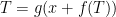 , where
  is the radiation’s temperature-independent component. That temperature-independent component may be, say, back radiation caused by carbon dioxide that we’ve placed into the atmosphere by burning fossil fuels.
 and
and  ? I don’t know. But let’s assume some functions that don’t ignore dependence on the entire temperature, and let’s observe how that constrains sensitivity. We’d expect temperature to be less dependent on temperature as temperature increases, and modelers who talk about things like tipping points obviously expect back radiation to become increasingly dependent on temperature as temperature increases. So let’s say for the sake of discussion that the functions take the following forms:

 ,
,  ,
,  are arbitrary constants.
 is all the radiation, not just
  is the whole temperature, and
  responds to all of it.
 ,
,  , and
, and  . If we employ the inverse function
  of the resultant relationship
  on Lord Monckton’s assumed “emission temperature”
  244.6 K, we get a temperature-independent radiation component
  , which we’ll take as our value for insolation after albedo. If we then solve the feedback equation
  for that value we get
  . That is, this model does exhibit a “substantial feedback response”
  to the emission temperature: it exhibits the response that Lord Monckton says the mainstream climate models lack.
 of CO2-caused back radiation to the
  of insolation to obtain a higher value
  . Solving the feedback equation
  with this increased temperature-independent radiation component
  gives us Lord Monckton’s pre-industrial temperature
  .
. of “forcing.” \textit{Forcing} is an initial radiation imbalance that would result from suddenly making a given CO2 concentration change. We make an estimate
  of the temperature change needed at the effective emission altitude to cause that radiation change, and we obtain the surface radiation change
  needed to cause the same temperature change at the surface. By solving
  we obtain a sensitivity
  .
.
Thank you for consistently pointing out Lord Monckton’s central error: although he says he knows the system has nonlinearities, he betrays no understanding of what the implications are.
Lord Monckton has not provided a scintilla of evidence for the remarkable proposition that the dependence on temperatures below the “emission temperature” of things like atmospheric water-vapor concentration and albedo from snow cover escaped all modelers’ notice before he discovered that dependence. His whole theory is based on confusing small-signal quantities with large-signal. The sensitivities at which they arrived can easily follow from positive-feedback assumptions in which that purportedly overlooked dependence is taken into account.
Let’s suppose for purposes of discussion that under the conditions modelers assume in this context the solution to the model equations results in some equilibrium relationship
Let’s also say that the radiation
What is the nature of the functions
and
where
Now, you may think that such relationships are much too simple and imply much greater sensitivity than the evidence supports. I agree; I don’t for a moment think that such relationships are valid. But that’s neither here nor there. What’s important to the present discussion is that they don’t ignore, as Lord Monckton contends that climate models do, the portion of the temperature value that’s less than some “emission temperature”:
Let’s suppose that
Since this model doesn’t lack that response, let’s determine whether recognizing that “substantial feedback response” has caused the model’s equilibrium climate sensitivity to be low. To do that we’ll first add
“Equilibrium climate sensitivity” is the change in equilibrium temperature caused by a doubling of CO2 concentration, and doubling that concentration is said to result in
In other words, climatologists are perfectly capable of arriving at a high sensitivity even if they take the entire temperature into account, i.e., even if their models provide “substantial feedback response.”
Mr Born characteristically mischaracterizes what I have said when he says: “Lord Monckton has not provided a scintilla of evidence for the remarkable proposition that the dependence on temperatures below the emission temperature of things like atmospheric water-vapor concentration and albedo from snow cover escaped all modelers’ notice before he discovered that dependence.”
I have said nothing about “temperatures below the emission temperature”. I have said – and Mr Born appears to agree – that emission temperature itself, and not some lesser quantity, induces a substantial feedback response.
I have also said, contrary to Mr Born’s characteristic mischaracterization of what I have said, that modelers do take the feedback response to emission temperature into account: but I have argued – and Mr Born’s own figure-work tends to confirm that I am correct – that they take insufficient account of it.
I even cited Lacis et al. (2010), and stated that their figures imply an 8.7 K feedback response to what Mr Born characteristically mischaracterizes as my “assumed emission temperature”.
Mr Born may not be familiar with the fundamental equation of radiative transfer: so let me explain that at Lacis’ stated albedo 0.418 and at today’s insolation that equation yields an emission temperature 243.3 K. That is not “assumed” by me: it is the ineluctable consequence of Lacis’ stated values of insolation and albedo.
Next, Mr Born again characteristically mischaracterizes my words by saying that the feedback response to emission temperature had been “purportedly overlooked”, when in fact I had said it had been undervalued, giving Lacis an example.
Mr Born then sets out a calculation based on a further characteristic mischaracterization of what I had said. He says I had contended that the climate models had ignored “the portion of the temperature value that’s less than some emission temperature”. No: I had said that the models had undervalued the actually large feedback response to emission temperature – a feedback response similar to that which Mr Born himself calculates.
In his model, emission temperature is 246.6 K and it induces a feedback response of almost 20 K, or two and a quarter times the 8.7 K implicit in Lacis (2010). But even that feedback response is far too low to be realistic.
It would imply the following apportionment of the 41 K difference between Mr Born’s 246.6 K emission temperature and the surface temperature in 1850:
19.8 K feedback response to emission temperature; 54.5 / 3.7 = 14.7 K directly-forced warming from adding pre-industrial CO2 to the atmosphere; 0.0 K directly-forced warming from any other greenhouse gas; 6.5 K feedback response to the direct forcing from CO2. Assuming a constant feedback fraction, the feedback fraction would thus be 1 – (244.6 + 14.7) / 287.6 = 0.1, little different from the values considered in my various articles, but only one-sixth to one-seventh of the 0.67 or 0.75 posited by CMIP3/5 and by Lacis respectively.
On the other hand, suppose that one were to use official climatology’s form of the zero-dimensional-model equation on Mr Born’s results. Then the forcing and feedback attributable to CO2 would add 14.7 + 6.5 = 21.2 K to global temperature, whereupon the feedback fraction would be 1 – 14.7 / 21.2 = 0.31. Even that would imply a Charney sensitivity of 1.6 K, or half of the 3.25 K Mr Born would like us to imagine. But then one would have to explain what ultra-extreme nonlinearities subsist in the feedbacks that would allow a feedback response amounting to only 8% of the emission temperature, followed by a further feedback response suddenly amounting to 46% of the directly-forced CO2 warming.
My point is this. The larger the feedback response to emission temperature, the less room there is for a large feedback response to the addition of the naturally-occurring, non-condensing greenhouse gases, whereupon Charney sensitivity will be very considerably below its current value.
Joe
I remember reading the history of GCM development, they had a problem making the models warm enough, they ran cold.
They fixed it in the parametization of the water/air boundary layer by allowing the supersaturation of water in this layer. After which models ran hot, and they used aerosols to tune the output to match history.
This is documented in the ModelE TOE, and it’s listed here in the CMIP doc’s, They just changed the name a little and called it mass conservation. This allows them to get the water forcing they need to get the GCM to run warm enough.
http://www.cesm.ucar.edu/models/atm-cam/docs/description/node13.html#SECTION00736000000000000000
Also at issue is on top of your feedback response, there is also a response from water vapor. And this is what I’ve been going on about for a year and a half about. They include positive water feedback as it warms, but this is a dynamic system they may or may not have modeled, and every night it cools, this puts a limit on how much water is left from the positive feedback, what I discovered (as a few other have), is without water vapor, surface temps would be much colder. But water vapor created in the tropics is distributed by air currents, and some as clouds.
But water vapor stays vapor based on surface pressure and temp. As it cools at night the water vapor in the entire atm column also has to cool (you can see how much changes by comparing daytime vs nighttime lapse rates), as the air cools below the 100% rh, water has to condense (you can also include the quantum probabilities of some condensing below 100%). But the heat of evaporation of water vapor from the state change is a lot more than just cooling the vapor cloud by 1 degree, it’s 4.21J/g vs 1J/g, which has to be released as IR.
So as the column cools, it generates it’s own self heating IR emission, where 1g condensing prevents ~4g from cooling 1 degree. As with co2 back radiation, this radiation is omni directional, some up, some down. And there’s a lot of it.
At the same time from the surface, even if the 15u band is blocked, the optical window it’s, and represents about 40% of the SB power spectrum, So if the surface to sky SB equation is equal to 80W/m^2, 35W/m^2 is bleeding out through the optical window, even if the other parts of the band are “block”.
Yet it is under these conditions, where at dusk it’s cooling 3 or 4F/hr, at 4am as air temps near dew point it slows or stops cooling, while still clear and calm out (I know because I’m taking pictures of galaxies).
So there’s a conundrum, it’s stopped cooling while at the same time there is a hugh energy hole still opened to space.
What I discovered is it’s the IR from the stored latent heat of evaporation, that has “gain” (4.21J/1J) that radiation supplies the energy that is bleeding to space. But it only has to condense enough to keep air temps at the surface above dew point, so surface temps slow or stop dropping, and just enough water vapor condenses to account for this.
This is what the signals looks like. Yes I show this 1,000 times, but it is proof it’s game over to this mess.
Micro
I dont see the si units on the bottom of your graph?
The units are listed on the right side in the legend. Degrees F , W/m^2 , RH %
eishhh
F (degrees) is not SI
anyway
my results om global T Min. show that vegetation traps heat.
More vegetation => higher Tmin
[remember that Tmin would be measured sometime at nighttime, so you cannot compare this with any measurements taken during the day.]
As long as its minimum it works. I do a number of different ways to look at the data. This was over grass. F allowed for a single scale. What I found for grass is it acts as an air gap insulator, below tree canopies would do the same. While bare ground is much warmer than grass. My interest was (nighttime) cooling rates.
And this was from someone else’s paper, but I’ve replicated it locally (other than net radiation), while also measuring Tzenith and doing SB calculations.
How tediously predictable. It serves no purpose to set right all the misstatements and distortions in Lord Monckton’s comments. I’ll limit myself to the main one and then return to something less painful: doing may taxes.
As usual, Lord Monckton says one thing in his posts and argues something else in response to analysis. Now he says “I have said, that modelers do take the feedback response to emission temperature into account: but I have argued – and Mr Born’s own figure-work tends to confirm that I am correct – that they take insufficient account of it.”
But what he said before I illustrated the nonlinearity’s implications was this:
Lord Monckton doesn’t discuss honestly. He consistently indulges in what it has become fashionable to call a “motte and bailey” argument. He started out saying his twelve years of Herculean effort uncovered a fundamental omission. In responding he now says merely that no, he never meant the models omit the effect; he was only saying they didn’t get the magnitude quite right.
Parturiverunt montes, natus est ridiculus mus.
Only now does the Born Liar reveal that his snide, arrogant and mendacious personal attacks on me in this thread are not attacks on the present head posting, or on any of the pieces in the present series, but on my response on another blog altogether to Dr Spencer, who considers that no allowance whatsoever should be made for even the smallest feedback response to emission temperature.
The Born Liar knows perfectly well that, throughout the pieces here, I have been citing Lacis et al. (2010), where an 8.7 K feedback response to emission temperature is implicit. And, in a previous piece, I had invited answers to the question what this 8.7 K was, if it was not a feedback response to emission temperature. But the Born Liar, in his petty determination to make out that we are incorrect when he is beginning to realize that we are right, resorts to his favorite technique – outright fabrication. He ought to be ashamed of himself, but is too stupid.
My, my, Lord Monckton does go on, doesn’t he? I won’t respond to his incoherent sputtering, but I will comment, because something serious is at stake. , i.e., the temperature without back radiation or feedback, is 255 K. If insolation net of albedo is
  , that temperature implies an open-loop gain
  . He also read that without feedback the pre-industrial back radiation
  from naturally occurring non-condensing greenhouse gases (“NOGs”) would have added only another
  . Taking the pre-industrial temperature with feedback to be
  , he solves the feedback equation
  for loop gain
  (which he calls
  ) to obtain the modest loop-gain value of 0.08.
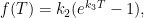
 above the emission temperature: they instead solved
 ![T_N=[R_{sun}+R_{NOGs} + f(T_N-T_E)]g](https://s0.wp.com/latex.php?latex=T_N%3D%5BR_%7Bsun%7D%2BR_%7BNOGs%7D+%2B+f%28T_N-T_E%29%5Dg&bg=ffffff&fg=000&s=0&c=20201002) to arrive at a substantial loop gain of 0.75:
to arrive at a substantial loop gain of 0.75:
His brief dedicates paragraphs 23-40 to a prolix presentation of the following argument. Not only will the excess verbiage annoy the court but there’s a real possibility that the judge or one of his clerks will detect how mathematically incoherent it is. This risks painting all skeptics as deluded lightweights.
Lord Monckton’s argument is simple. But by leaving open-loop gain (as opposed to just plain loop gain) only implicit he perhaps obscured the degree to which it relies on linearity. So I’ll paraphrase his argument with open-loop gain expressed explicitly.
Lord Monckton read that the emission temperature
Although he now seems to be back-pedaling, he contended in his amicus brief that prior to his insight all climatologists had instead computed the feedback relationship by assuming it responded only to the temperature portion
Lord Monckton is no doubt correct that the models end up making feedback more responsive to temperature changes at high temperatures than at low temperatures: they’re non-linear. But that’s far from the same as assuming “that the feedback response to the emission temperature of 255 K was nil, while the feedback response to the next 8 K of temperature caused by the direct warming owing to the presence of the naturally-occurring, non-condensing greenhouse gases, was 24 K.” And it makes no sense to assume linearity to demonstrate that.
I urge Heartland to resubmit its brief with those paragraphs omitted.
Joe: I don’t think much of Lacis’s paper or any attempt to quantify the GHE for a planet with no GHGs or just WV. The GISS is parameterized/tuned to reproduce today’s climate. IMO, it is absurd to assume that those parameters are relevant to modeling a radically different planet. Every time I read about 33 K, I retch. We know that GHGs and clouds reduce outgoing LWR from about 390 W/m2 to 240 W/m2. That 150 W/m2 is the GHE. Doubling CO2 is good for another 3.5 W/m2 of enhanced GHE. The tough problem is converted change in radiation into changes in temperature. If we knew how to do that, we would know climate sensitivity. The IPCC says there is a 70%? likelihood ECS lies between 1.5 and 4.5 K. In other word, we really don’t know how to convert a change in W/m2 into a change in temperature. So I think of the GHE and e. GHE only in terms of W/m2
Frank:
I didn’t read Lacis, but that 255 K number seemed bogus to me, too. As I said, I was just spit-balling the toy model I set forth upthread, but I used a lower value there.
On the other hand, I picked a significantly higher number out of the air for pre-industrial surface radiation; your 390 W/m^2 seemed to me to assume a uniform 288 K, so I raised it an arbitrary amount (I pulled 18% out of the air) because of non-uniform temperature.
In answer to Mr Born, Heartland has not submitted a brief to the California court. And, whether he likes it or not, official climatology defines a feedback as a process responding only to a change in temperature, and not to a pre-existing temperature.
I have been morbidly fascinated at how the discussion has endlessly conflated (1) what the IPCC may define as feedback with (2) whether the models’ differential equations make surface radiation or forcing respond to temperature throughout the temperature range.
Different issues entirely.
Joe: Your April 6, 2018 at 8:51 am comment assumes that the Earth behaves like an amplifier. You’ve got the wrong physics – even though the equations are the same in some cases. Climate is not an amplification system, but the equations can be manipulated to make it look as if it were.
dW = λ*dTs λ = dW/dT
When the Earth warms, it emits more LWR to space and may reflect more or less SWR back to space. dW is that total change. It is heat lost (a negative quantity) making λ negative,
If the Earth were a simple graybody at 288K and e = 0.615, dW/dT would be -3.3 W/m2/K. This is called λ0. It can also be calculated with AOGCMs with temperatures that range from 190-310K by simply raising the temperature 1 degC everywhere (or with more sophisticated methods). AOGCMs say λ0 = -3.2 W/m2/K. The simple gray-body model is a good one in this case and much simpler to understand.
As the planet warms, more water vapor in the atmosphere slows down radiative cooling to space. More water vapor lowers the lapse rate, meaning it warms more high in the troposphere than at the surface. That increases radiative cooling to space. Clouds may change in both emission and reflection. Changes in seasonal snow and sea ice will change reflection through clear skies. All of these changes modify the simple gray-body relationship between the increase in temperature and the increase in radiative cooing to space. Sometimes climate scientists talk about λ_vw and λ_lr and λ_clouds and λ_ice. However, all we need to do is sum all of these feedbacks up to λ1. Now:
dW = (λ0 + λ1)*dTs
None of this really accomplishes anything important, because we have no way of observing λ1 (or λ0). These values all come from inadequate MODELS. You may as well rely on λ produced by that model. It is much simpler. To eliminate a radiative imbalance caused by a forcing, dF, we need an increase in radiative cooling to space so that dF + dW = 0. Substituting and rearranging:
dTs = -dF/(λ0 + λ1) = (dF/λ0) * (1/(1+λ1/λ0) = T0 * (1/(1-f))
This is an equation used with amplifiers and control systems (and I don’t understand them). Now we have made global warming APPEAR to be a no-feedbacks warming (T0) is amplified by feedbacks (except by “Planck feedback” which produces T0). Have we accomplished anything by this exercise. No! Without λ1, we don’t know λ. And λ is all we need to know: dW = λ*dTs. ECS is F2x/λ. All we have accomplished is given alarmists a way to scare us (AMPLIFICATION BY FEEDBACKS); and Monckton an opportunity to screw things up ignoring that dW many not change linearly with dTs. And by confusing dTs at equilibrium with current transient dTs.
Actually, sophisticated climate scientists can use this analysis. Absolute GMST (not anomalies) 3.5 K every year, giving us a way to OBSERVE dW/dT = λ from space. And we can measure λ in both the LWR (thermal emission) channel and SWR (reflection) channel. And we can look at clear skies (where only WV + LR feedbacks operate) and the difference between clear and cloudy skies (cloud feedbacks). And we can compare the predictions of models to observations from space and learn that models are pretty bad – and mutually inconsistent. See: Tsushima and Manabe (2013) PNAS. IMO, the data in this paper reveals more than any other how our planet really behaves. But seasonal warming is not global warming – it doesn’t provide all the answers. In particular, reflection of SWR doesn’t respond linearly to a rise in Ts during seasonal warming.
Frank:
That comment is puzzling; all I did derive the relationships you presented yourself. Therefore, if I’m assuming the earth behaves like an amplifier and have thereby gotten the physics wrong, you did, too.
Actually, I’m happy to say that the earth behaves like an amplifier; if the same equations apply (and for small enough signals they have to), then to me that’s behaving like an amplifier. I think a lot of people on these threads have gotten hung up on other things we ordinarily associate with electronic amplifiers, such as typically greater available power out than in. But the equations we’re dealing with don’t reflect that. More-detailed amplifier equations would include things like input and output impedance and load, and available power would thereby be implied, but the amplifier equations we’re invoking here don’t do that.
An amplifier equation, for example, may determine voltage out for voltage in. Without impedances, loads, etc., that says nothing about adding power. The analog in climate is power density in and temperature out. Again, nothing there about adding power. Yet people on these thread keep going on about how the earth isn’t an amplifier.
In a sense it isn’t, but how is that relevant to anything we’re discussing? Amplifiers come into the discussion only to the extent that the equations we are using for simple climate models are also used for simple amplifier work. Whether the earth is an amplifier is irrelevant.
Joe: My derivation didn’t include heat capacity, because I implicitly assumed dT was at equilibrium and no heat was flowing into the system. I was confused when you started with a complex (heat) capacity. Then you started to discuss open loop gain and other aspects of amplification I’ve never mastered.
Why avoid the amplifier analogy?
I don’t know anything about non-linearity in amplifiers, but non-linearity quickly becomes an issue for warming.
Amplifiers require an external power source; amplification of warming by feedbacks doesn’t appear to. (In reality, larger feedbacks mean that the radiative imbalance lasts longer before equilibrium is reached, so the sun is the external source of no-feedbacks warming and amplified warming. Many don’t understand this, so it looks like a violation of CoE.)
Avoiding f means that everything is measured in W/m2/K: λ, λ0, λ1, λ_wv, λ_lr, λ_swr, λ0_cloud_lwr. Every one of these terms has a PHYSICAL REALITY associated with it: the change in net flux to space per degK of surface warming. The feedback factor f does not have a physical reality. Feedback is a “response” to change, not something that must cause amplification.
What does it mean for the f to approach one? I don’t know. However, if the sum of of all feedbacks is near zero, then the planet can warm without emitting+reflecting any additional energy to space, a clear physical explanation for a runaway GHE. What happens when λ gets very large? It is very hard for a forcing to change the temperature, because it takes very little surface warming to radiate away a lot of power.
Simple gray bodies have λ = 4eoT^3 unless you treat emissivity as a variable: λ = 4eoT^3 + eoT^4*(de/dT). If you think of the planet as a giant black box – or better, a gray box – LWR feedbacks are equivalent to a change in emissivity with temperature. SWR feedback is a change in absorptivity (or albedo) of the fray box with temperature.
Best of all, I don’t need to learn about electronic circuitry. Radiation physics is simpler.
Frank: , and there’s no reason to use amplifier terminology. But it would still make it easier for slowpokes like me in your audience if you’d provide a canned introduction of your notation when you write that kind of stuff.
 in response to a constant (input) radiation density
  . If a small departure
  occurs from that reference radiation density
  , the response is a departure
  from
from  given by
 is heat capacity per unit area and
  and
and  are are temperature-responsive additions to the original perturbation. If
  , i.e., if the response to temperature is negative, then a new equilibrium (
 ) state is established:
 "
"
You’re probably right to avoid Lord Monckton’s
You could start off like:
“A system is initially at equilibrium, exhibiting a constant (output) temperature
“
where
"
. . . and so on.
For large departures, you can make it non-linear as I did in my toy model above.
You thus avoid using amplifier nomenclature if you want, but you'll be making clear what everything means.
As I said before, though, that stuff about amplifiers needing an external power source is a red herring; the amplifier equations people are using for this purpose deal with quantities other than power.
Joe, you said “……about amplifiers needing an external power source is a red herring; the amplifier equations people are using for this purpose deal with quantities other than power.”
Don’t you think Frank was talking about an electrical circuit (an amplifier) needing to be connected to an external “Power Supply” like with a transformer, fuse, diodes, filter capacitors (or batteries) – not “power” in the sense of Watts?
An op-amp for example is usually drawn as a triangular three terminal device, a (+) input, a (-) input, and an output. It is understood (seldom shown) that the IC chip (usually 8 pins total) requires a bipolar supply like +15volts and -15volts using two more pins. They have to be “fed” of course (active), and this is a valid point Frank makes – possibly making an amplifier quite different from a climate process.
Lord M
I am truly surprised with your reactions to Michael Moon.
He was offering you support for research and you completely ignored him or took him up on his offer. Instead you challenged him on his comments…
That seems really dumb to me?
You’ve missed CM reply dated March 30, 2018 at 5:31 am
Bob
the dates are not right
look at this comment
https://wattsupwiththat.com/2018/03/30/game-over/#comment-2779191
and the one below.
There is no response from Lord M
I believe he mentioned being ill
It could be more serious than we think?
It is no business of the furtively pseudonymous “henryp” to lecture me on whether I should accept an imagined offer of funding from someone else posting here. For the avoidance of doubt, nobody funds me to conduct climate research.
Lord Monckton or should I say Lord Monster?
I find this remark a bit impolite
I thought Mr.Moon’s offer was genuine but maybe I was a bit naïve. He did not repeat his offer. The Lord knows, you are going to need some help if you want to actually prove that a change of 0.01% in the atmosphere can change the weather on earth. In this respect the debate has not changed much in the past 10 years. Even in those days I said that you cannot ‘calculate’ that which has never been measured. We all know that the IPPC put the cart before the horse in this respect.
Anyway, if you want to know my name you can just click on it and find the charities I am involved with. I also work Pro Deo for these two charities;
I am a pensioner.
The furtively pseudonymous Henryp wonders why I reply so seldom to anything he posts. The reason is that it is nearly always off topic, and nearly always error-laden.
On any view, it was none of his business to lecture me on whether I should accept a half-assed offer of funding, for a project other than and incompatible with that in which I am engaged, from someone on a thread here who was claiming to be wealthy.
And at no point have I asserted that I wish to prove that an alteration of one part in 10,000 in the atmospheric composition will change the weather on Earth. I have stated, time and again, that for the sake of argument we are accepting all of official climatology except what we can prove to be wrong.
If Henryp is unfamiliar with the logical modes of argument in science, such as acceptance of an opponent’s premises ad argumentum or ad interim or ad experimentum, then I suggest that he obtains some elementary instruction in the philosophy of science.
Monckton of Brenchley at April 3, 2018 at 7:47 am concluded a comment with:
“My point is this. The larger the feedback response to emission temperature, the less room there is for a large feedback response to the addition of the naturally-occurring, non-condensing greenhouse gases, whereupon Charney sensitivity will be very considerably below its current value.”
No Kidding ? If it were not so large – it would be smaller!
There has been here considerable (trivial to engineers) discussion of a first-order feedback system. The system is 100% clear as electronics – far less clear as a climate model.
We considered an amplifier with gain A that has a first-order feedback loop f around it. For an input X and an output Y,
Y / X = A / (1 – Af)
For example, if we know A, f, and X, we can compute output Y. Given any three of X, Y, A, and f, we trivially compute the fourth. If it is a desired ratio Y/X we would like to end up with, we can find an infinite array of values of A and f that satisfy this. With electronics, we know things rather exactly (we set it up). With climate – do we know any of Y, X, A, or f at all well?
One can realistically conclude that the Charney sensitivity is lower than claimed based on observation alone. Arguing errors in setting the input parameters to a slippery feedback model (that may not even be significant – f is very small) proves little.
With regard to the engineering modeling, Mr. Monckton did not understand it (gain for stability can approach f=1, amplifier gain could be A=1, modern flow-graph rendition). There is nothing wrong with being wrong, if one can learn. In such an instance, it is proper to admit error, thank the teacher, and move forward. In such an instance, (while claiming contrary to one’s own writings that one did already know something), lambasting the instructors (“ape-like, children’s arrows, Party Line, Socialist training, hate speech, whose ignorance is as bottomless as his arrogance, his dishonesty, overwhelmingly totalitarian”) is inappropriate, to say the least.
Mr. Hutchins:
Don’t expect common courtesy, or even honesty, from Lord Monckton. I’ve more than once tried to throw him a line when he was clearly in over his depth. His behavior was always puerile.
On another subject: You may be interested in the characteristics of the (totally made-up) nonlinear system I described above. My nomenclature may seem odd, but it’s what they used when I had clients dealing with this stuff. “Open-loop gain” is gain before feedback, “feedback gain” is the gain of the feedback block, just plain “loop gain” is the quantity whose small-signal value Lord Monckton refers to as “f”, and “closed-loop gain” is gain after feedback is connected in.
The system is not intended to accurately represent anything in the real world; I just wanted a sample non-linear system to illustrate the difference between large- and small-signal values of various quantities.
Now let’s see if I can put an image here:
http://i64.tinypic.com/1t3p4x.png
Mr Born, or the Born Liar as he is now known, continues to be arrogant, impolite and wrong. However much he may expatiate on the virtues (if any) of his own model, the ineluctable fact remains that if one makes due allowance for the feedback response to emission temperature the feedback fraction will be less than if one does not. Official climatology does not.
Mr Hutchins continues to state, falsely, that I do not understand that a feedback fraction can approach unity in a stable regime, when in fact I have patiently tried to assist his limited knowledge of this subject by explaining that designers of electronic circuits manufactured with variable componentry and intended to run in a variety of operating conditions will typically design the circuits so that the feedback fraction does not exceed 0.1. As it turns out, once one allows properly for the feedback response to emission temperature, the feedback fraction in the climate is of order 0.1, which is no doubtone of the reasons why global mean surface temperature has varied by only 3 K either side of the 810,000-year mean.
Mr Hutchins continues to state, falsely, that I do not understand that the open-loop or direct gain factor in an amplifier gain block may be unity. Of course I understand that: for we not only built our own test rig precisely to model that condition, among others: I also commissioned a government laboratory to do the same. Mr Hutchins has already been told this: but, in his desperation to make out that I don’t know what I’m talking about, he now resorts to outright lying. That is not acceptable.
If Mr Hutchins continues to misrepresent me, I shall continue to call him out as the liar he is.
Mr. Monckton perhaps does not realize that in a teaching career an instructor has suffered hundreds of instances of students complaining that they should have gotten more credit on an exam problem. The approach and phraseology are familiar enough. Having examined the published solution, and studied their error, they come in with a generally warped theory that what they wrote on the test really indicated exam-time understanding! Almost always (as is the case with Mr. Monckton) such excuses retain a residual but distinctive traced of the original misunderstanding (as when Mr. Monckton, being told by me that A obviously could be 1, did not simply say that he had learned something, OR even that he knew it all along, BUT rather he said: “That’s not quite the same as building a feedback amplifier with a gain block whose gain factor can be set to unity.”). If he understood, he would know it is EXACTLY the same thing. No shame in learning something.
Mr Hutchins continues to try, futilely, to misrepresent me and then to imply that it is only through his wisdom that I was corrected. Not for the first time, he is lying, and nothing more than that needs to be said.
Dear Lord Monckton,
Sorry for the my late reply. I am guessing that probably some others will have already mentioned this as I find it very obvious, but in case they haven’t, I feel that it must be said.
While I find impeccable your logic that any positive climate feedback that may exist should be also working on the base emission temperature, and that this is an important flaw in the currently mainstream way of calculating it, I disagree with the numbers themselves. My main disagreement is with the feedback value being a constant. I believe that it can probably be aproximated by a constant over short temperature ranges such as the ones experienced by our wonderful planet due to GHGs, but I would not expect that it would stay with the same value for all the temperature range back to 0 Kelvin. I believe that the value of the feedback “f” when changing the emission temperature from X Kelvin to X+Y Kelvin with Y<<X is a function of X. So basically I don't think that you can use the same "f" that you use for today's variations in temperature caused by greenhouse gasses alone, to the base temperature itself. The feedback mechanisms present at 287K due to adding a degree or two are simply completely different to the ones that you would have at 50K due to adding a degree or two, but when using the same value of f your paper assumes that the feedback value stays constant for all the temperature range.
IMO the correct feedback value to use for the base temperature would be the result of integrating the variable f(X) accross the temperature range from 0K to the base temperature. But who knows what the real function of the feedback looks like. It could end up happening that this value is similar to the current feedback value, or it could be very different. Frankly I have no idea what it could be. I do know however that the assumption that it is the same needs to be proven.
Best regards.
In response to Nylo, once one accepts that the emission temperature induces a feedback response, the interval across which nonlinearities in feedbacks might obtain is reduced from the 33 K commonly talked of to about 9 or 10 K. Besides, the response to the water-vapor feedback is linear or very close to it, as I shall discuss in a future posting. Besides, if official climatology has hitherto been either ignoring outright or grossly undervaluing the feedback response to emission temperature, then such nonlinearities as are thought to generate the current climate sensitivity will still be present, but climate sensitivity must nevertheless be significantly below current estimates.
In fact, as the next posting in the series will reveal, calibration of the zero-dimensional-model equation will demonstrate that, though it is explicitly linear, it reproduces exactly the interval of Charney sensitivities predicted by the last two generations of general-circulation models, which expicitly take nonlinearities into account.
Finally, it is not particularly difficult to prove that the mean feedback fraction applicable to the emission temperature is the same as the mean feedback fraction applicable to any enhancement of that temperature. The relevant equations will be presented in a follow-up post.
Frank
A careful analysis, results here,
https://wattsupwiththat.com/2018/03/30/game-over/#comment-2778501
of 11 weather stations in my own country showed that the increase in CO2 gave me a negative result.
However, if we assume that CO2 doubling gives ΔT_0 =0.00
then we get:
1) A doubling of CO2 creating a 0.00 rise in temperature.
2) A 0.00 rise in temperature creating an additional 0.00 rise in temperature due to feedbacks.
3) That 0.00 in temperature creating an additional 0.00 rise in temperature due to feedbacks.
4) 3) 0.00 rise in temperature creating an additional 0.00 rise in temperature due to feedbacks.
5) And so on.
I think that makes everything perfectly clear to me and everyone else as well?
Obviously, if the result is negative, as I expect, your formula is not going to work…
HenryP: The data you cite is inconsistent with the rising temperature observed globally: 1) with traditional thermometers 2 m above the ground, with satellites detecting microwaves from the troposphere, with SST measured by a variety of techniques and now with 4000 ARGO buoys sampling the ocean at various depths using one technology. All of the temperature records have problems: Reliably detecting changes on the order of 0.1 degC per decade is extremely challenging. The net correction made to the surface temperature record add only 0.2 degC. This doesn’t mean that the records you cite are wrong or right – they just disagree with what is reported globally. (You can look up your local stations and other near stations and see how BEST – originally a group of skeptics funded by the Koch Brothers – processed ALL the data from your region.)
http://berkeleyearth.lbl.gov/city-list/
During a strong El Nino, GMST can rise almost 0.5 degC in six months and fall 0.5 degC in the following six months. How can this happen? There is a massive amount of very cold water in the deep ocean that sank in polar regions. Some of this very cold water upwells in the Eastern Tropical Pacific because trade winds blow water from east to west, stimulating upwelling. As that water is swept across the Pacific it warms and then sinks in the Western Pacific. However, when those trade winds slow (and sometimes reverse) upwell of cold water and sinking of warm water slows and the whole planet warms as heat from the warmer Eastern Pacific is spread across the globe. This is called natural variability. Heat is irregular redistributed from one location on the planet to another by chaotic ocean currents and winds. As a consequence, all of the alarmists who cite a decade or two of warming and all of the skeptics who cite a decade or two of cooling of Pause could be drawing conclusions from natural fluctuations in the transfer of heat WITHIN our climate system. These conclusions may have nothing to with an IMBALANCE of heat transfer by radiation at the top of the atmosphere. Both sides are exaggerating the importance of difficult measurements of local warming and cooling. Only global changes over the last half-century or so are meaningful to me. Everything else is weather, not climate. FWIW.
frank
My Rule no. 1: I decided to look at the change of weather (temperatures), rather than absolute temperatures.
As an example I attach my [separate] result sheet for George (South Africa).
My original data come from http://www.tutiempo.net
I specifically used the data from this website as I distrust the various Anglo Saxon websites, like BOM, NOAA, Best, etc.
You can type in the city that you are interested in and search the website.
As an example take the case of George, South Africa. the link to the original data is here:
http://www.tutiempo.net/clima/George_Airport/688280.htm
It gives the average yearly mean, max. and min. temps, in that order, as per the first three columns.
I copied that data to my Excel sheet, as attached.
For the years with missing data (red), you have to go to the individual months and look at every month’s average. Click on the relevant (blue) year and chose the month.
(for the results: see far below in the attached file, 1983, 2002 and 2005)
[For months with less than 15 days data I applied the rule that I would rather take the average of
[same] month of the preceding year and the following year, thereby adhering to Rule no. 1]
Now you can do the least square linear regressions from at least 4 points. The overall result for George is an average decline of -0.0131K per annum since 1978, that is -0.5 degrees C, in total, since 1978, as shown (the value before the x)
By selecting different periods of data [in the graph] you can get the various inclines/declines from more recent times {i.e. the values before the x}, getting at least for 4 points for the speed of warming/cooling.
George is just one single result in my files. There is 54 in total.
Let me know if you there is anything that is not clear to you as to how I obtained the data.
The problem with your datasets is that they are properly not balanced NH and SH (equal amounts of stations SH and Nh & balanced to zero latitude and 70/30 @sea/inland.
Also, you cannot go more than 40 years back.
And the sats have problems of degeneration with the current scorching sun. It seems there is always a drift up…What version are we on now?
HenryP wrote: “As an example take the case of George, South Africa. the link to the original data is here.”
This almost certainly isn’t the original raw data, since that is monthly data.
HenryP wrote: I specifically used the data from this website as I distrust the various Anglo Saxon websites, like BOM, NOAA, Best, etc.
Henry, you can believe whatever data you want to, but scientists usually have good reasons for deciding what data to believe. About a decade ago, there was a lot of concern at skeptical websites about access to raw temperature data and how it had been non-transparently processed by GISS, NOAA, Hadley, etc. (See Climateaudit.org) In the wake of the Climategate email scandal, most of the raw data and software became freely accessible. Several prominent skeptics went back to the raw data and analyzed it from scratch using their own ideas how it should be done. The consensus of these skeptics was that the established records were about right.
The Berkeley Earth Project (BEST) was the most sophisticated of these efforts, with serious funding from the Koch Brothers and headed by a physics professor who had been publicly critical of the behavior of climate scientist revealed by Climategate. Instead of starting with the standard set of historical data, they started with as many temperature records and an novel way to process that data (kriging). They have tried to make their data and methods as transparent as possible. However, after their results agreed with the earlier consensus, they have come in for criticism mindless criticism.
I’m not telling you what to think, just where you might look for more information.
frank
If you go into the month you get the original daily data?
The data sets you prefer are not balanced NH and SH. They are all biased towards the NH.
There is no ‘global” warming. It is more on the NH. Not so much in the SH…
https://wattsupwiththat.com/2018/03/30/game-over/comment-page-1/#comment-2778024
Yes, HenryP. Everyone who has constructed a global temperature record has has to deal with the fact that there are many more thermometers in some regions than others. Some work with surface grids and average all the thermometers inside each grid cell. BEST using kriging. And they all deal with seasons, which are handled by anomalies. And station moves and incomplete records and changing time-of observation bias (which is huge in the US and I have personally explored) and unexplained breakpoints in data compared with nearby stations. However, all this massaging of data adds only about 0.2 degC of warming to the 20th century. BEST made an index from purely rural stations and it didn’t differ from all stations. UHI is real, but apparently not enough stations are affected to create a serious bias. There are also station siting issues, but Andy Watts project can’t tell us how siting has changed and biased the record. All we know about is today’s siting.
It is of course possible that you could uncover problems with data or find a new method to analyzed that data and come up with an answer for global warming that is different from the consensus. When you do publish, your results. Until then, recognize that an immense amount of work has gone into studying the problem (including work by some as skeptical as you) and no one who has tackled the GLOBAL problem properly thinks it isn’t warming. Many have found things to complain about, but haven’t produced a different useful answer.
f = 1 – Tref/Teq seems appropriate for conductive energy feedbacks because E ~ T (depending on Biot/Nesselt Number).
However, f = 1 – (Tref/Teq)^4 would seem more appropriate for radiative energy feedbacks where E ~ T^4. In that case, Charney Sensitivity increases to about 1.8K.
1.45 K < ECS < 1.8 K. No?
I can’t agree as the original pre industrial feedback already included the T^4 effect. You would be needlessly juicing f would you not?
Sailboarder is correct. The emission temperature itself is derived by the fundamental equation of radiative transfer, which is a fourth-power relation. And the Planck sensitivity parameter, the first derivative of that equation, which is important because equilibrium sensitivity has a squared dependence upon it, is expressible in a linear form as T / (4Q), where T is temperature and Q is radiative flux density.
Monckton of Brenchley April 5, 2018 at 4:28 am
Sailboarder is correct. The emission temperature itself is derived by the fundamental equation of radiative transfer, which is a fourth-power relation. And the Planck sensitivity parameter, the first derivative of that equation, which is important because equilibrium sensitivity has a squared dependence upon it, is expressible in a linear form as T / (4Q), where T is temperature and Q is radiative flux density.
As shown above the first derivative dQ/dT= 4σT^3, which is a cubic not linear.
Hiding the non-linearity by dividing by Q which is itself a non-linear function of T (a quartic) is inappropriate.
Phil – as for dividing by Q considered the engineer’s “classical sensitivity”
http://electronotes.netfirms.com/Sensitivity.jpg
in which case you ALSO multiply your derivative by T. This is the PROPORTIONAL local slope. This leaves just the number 4. That is, for example, increasing T by 1% increases Q by 4%. Now that’s neat enough.
The concrete Earth ( the one on which we live) does not have a Charney sensitivity aka ECS. It is the abstract Earth that has a Charney sensitivity. To debate the magnitude of the Charney sensitivity is to make application of the reification fallacy by treating an abstract object as if it were a concrete object.
Mr Oldberg continues to be baffled by the notion that adding greenhouse gases to our atmosphere will be likely to cause some real and measurable warming. However, as the head posting makes crystal clear, we have accepted all of official clim,atology for the sake of argument, except where we have proven that it is in error. Therefore we have accepted that there is a greenhouse effect, which cannot be airbrushed away by irrelevant waffle about the “reification fallacy”.
Are you accepting the greenhouse effect in reality, or just for the sake of argument?
Frank and arfur
I cannot find your relevant argument on re-radiation but I don’t think you understand it.
I am a chemist so I know about spectrophotometry. Try doing a test with a substance dissolved in a liquid that has a strong absorbance somewhere in the visible area and try to peep in the cuvette area to see what happens to the light going through the cuvette when you turn the knob to the wavelength where you want to measure? Do you see what happens? The light cannot go through the cuvette anymore (which is why in the old time we used the word extinction) and comes back, IMO 62.5% of the direction where the light came from. The rest is scattered in all directions. There is no ‘thermalization” : as long as you keep the light on it will keep not going through the molecule. There is no build up of heat in the cuvette. It is as if the molecule acts like a little mirror in the areas where there is absorption. Now try to understand what I have been telling to Kristi Silber
https://wattsupwiththat.com/2018/03/30/game-over/#comment-2779055
& arguments that follow below that comment.
HenryP April 5, 2018 at 1:16 am
Frank and arfur
I cannot find your relevant argument on re-radiation but I don’t think you understand it.
I am a chemist so I know about spectrophotometry.
You may be a chemist but your statements below indicate that you do not understand spectrophotometry.
Try doing a test with a substance dissolved in a liquid that has a strong absorbance somewhere in the visible area and try to peep in the cuvette area to see what happens to the light going through the cuvette when you turn the knob to the wavelength where you want to measure? Do you see what happens? The light cannot go through the cuvette anymore (which is why in the old time we used the word extinction) and comes back, IMO 62.5% of the direction where the light came from. The rest is scattered in all directions.
The light is absorbed and electronic excitation occurs, not reflected backwards and certainly not 62.5%.
There is no ‘thermalization” : as long as you keep the light on it will keep not going through the molecule. There is no build up of heat in the cuvette. It is as if the molecule acts like a little mirror in the areas where there is absorption.
No it is not like ‘a little mirror’, if there’s any elastic scattering it would be Rayleigh scattering which is very weak and in all directions. If the substance is not fluorescent then the excitation energy is transferred to the solvent and ultimately to the surroundings (which is the case for most substances).
Phil.
We all know you believe in your books but you have no experiments to prove anything.
In fact: let me challenge you on just proving that CO2 is cooling the atmosphere. It is just a simple experiment.
I realize that the concentration of the CO2 is not much, but we know that both CO2 and H2O (g) have strong absorptions in the 0-5 um range. So, if I can prove that H2O (g), i.e. water vapor, cools the atmosphere, I would have also proven that CO2 cools the atmosphere.
Equipment: IR thermometer, Hygroscope, polished black plate used as a colorimetric zero, exposed directly to the sun’s light
Weather: sunny, no clouds
Time of day: 1 pm
For a few weeks: measure both the humidity and the temperature on the exposed plate and tell me what relationship you find between the humidity in the air and the temperature on the exposed plate>?
What are your conclusions?
I like that Henry, might I also suggest add measuring Tzenith with your IR thermometer.
Help me out. Tzenith=?
On that clear day point your IR thermo straight up. A, There’s a NASA paper that says with calibration, that’s a good measure of total Precipitation water. Second, it’s measuring through the optical window (other than TPW), and gives you a place to reference your SB calculations to.
What I found is it is fricking cold, even on warm days (again depending tpw), and if you look at the spectrum, this gives up a decent TOA temp as seen from the surface. So at dusk when it’s cooling 4F/hr and you measure it, and again at 4 am when it’s dropped about the same as surface air temp has dropped, but it’s stopped cooling at the surface you realize more is going on than you thought.
henryp April 5, 2018 at 8:43 am
Phil.
We all know you believe in your books but you have no experiments to prove anything.
Which goes to prove you know nothing about me. For about 30 years I ran very well regarded international laboratories researching optical diagnostics and experiments using spectroscopy were a daily occurrence! Your statements regarding your knowledge of spectrophotometry are wrong and I corrected them, I can’t imagine why you’re trying to change the subject.
PHIL.
Our fighting on photometry is off topic.
I was trying to get you on topic.
I cannot imagine you ever acccepting a challenge for doing some simple testing…
to disprove AGW
you have nothing to contribute other than your support forAGW.
Phil. wrote
For about 30 years I ran very well regarded international laboratories researching optical diagnostics and experiments using spectroscopy were a daily occurrence!
Henry says
eissh
this is so sad
That sounds really pathetic to me. All that time wasted and considering all the optics you studied and you still not figuring out during that time that there never was a man made ozone hole neither that there is any AGW….
I blame you and your ilk for all the confusion caused.
Don’t think I will ever forgive you – unless you ask me.
Phil and others: I am also chemist. Your laboratory spectrometer uses a light source with a filament heated to several thousand degK by electricity. In the laboratory, you only need to worry about the absorption of IR by GHGs. GHGs also emit thermal IR towards the detector, but that signal is negligible compared with the signal transmitted through a sample (think T^4). What my chemistry curriculum didn’t teach me is the Schwarzschild equation for radiation passing through a medium where both absorption and emission are important. This is the case for the atmosphere. When I first saw this equation, many mysteries instantly disappeared. The incremental change in spectral intensity at any wavelength, dI, while radiation passes an incremental distance, ds, through a medium is given by:
dI = emission – absorption (+ terms for scattering if needed)
dI = n*o*B(λ,T)*ds – n*o*I_0*ds
where n is the density/concentration of absorbing/emitting molecules, o is the absorption cross-section (extinction coefficient) for the wavelength of interest, I_0 is the intensity of incoming radiation and B(λ,T) is the Planck function for the local temperature and wavelength of interest. If you ignore the emission term and integrate, you get Beer’s Law used with your laboratory absorption spectrometer. If radiation has come into thermodynamic equilibrium with the medium it is passing through, dI = 0 and I_0 = B(λ,T), which is of course Planck’s Law. The Schwarzschild equation is needed when such an equilibrium doesn’t exist and emission is important. This is the case for thermal IR in the atmosphere. There is no analytical solution for this differential equation, it must be numerically integrated over a path: from the surface to space for OLR and from space to the surface for DLR. In that case, n, o and T are not constants, but variables: n(z), o(T,P) and T(z). The absorption lines are broadened by pressure and Doppler, so o changes with altitude. And you must integrate over all relevant wavelengths to get power. When you hear the phrase “radiative transfer calculation”, that usually implies numerically integrating the Schwarzschild equation. Some aspects of that process are automated online here:
http://climatemodels.uchicago.edu/modtran/
Planck’s Law was derived for radiation in EQUILIBRIUM with quantized oscillators, not real molecules. “Einstein coefficients are used in QM to describe the probability of emission, stimulated emission and absorption of photons by real molecules. Those coefficients lead to absorption coefficients used in spectroscopy. Emission coefficients are related to absorption coefficients through the Planck function B(λ,T).
If you are seriously interested in this field, I strongly recommend Grant Petty’s textbook, “A First-Course in Atmospheric Radiation”. It is written for meteorology students and says ABSOLUTELY NOTHING about global warming. The paperback is now $48 new and $32 used. Climate change has been my hobby for about a decade now, and this is by far the most useful book I own. You could read scienceofdoom.com from beginning to end, but most people think the host is a supporter of the consensus. (He is merely a supporter of consensus physics and you deduced ECS from that.) It took me about a year after Steve McIntyre recommended SOD for me to finally recognize that the host was merely trying to accurately present the physics of climate.
https://www.amazon.com/First-Course-Atmospheric-Radiation-2nd/dp/0972903313/ref=sr_1_1?ie=UTF8&qid=1522952766&sr=8-1&keywords=a+first+course+in+atmospheric+radiation
Frank:
You seem to have looked into a subject about which I’m almost totally ignorant, so maybe you can answer two questions:
1) Is there a reliable expression for forcing as a function of CO2 concentration that is good down to zero? (I know you want to say buy the book, but unless I weaken I’m going to resist that temptation.)
2) For concentrations within an order of magnitude or so of our current CO2 concentration, the value of forcing for a given CO2 concentration-change ratio doesn’t seem too controversial (right?). But it seems to me that obtaining that value would have involved performing quite a complicated calculation over disparate conditions at different latitudes. Do you know whether there have been many independent determinations of that value? Or has there been just one that everyone uses because he doesn’t want to expend the required independent effort?
Joe Born asked: 1) Is there a reliable expression for forcing as a function of CO2 concentration that is good down to zero? (I know you want to say buy the book, but unless I weaken I’m going to resist that temptation.)
Grant Petty is interested in the real atmosphere, so he doesn’t discuss variation in CO2 (IIRC). That is climate change, not meteorology. You can obtain some idea about the linearity of forcing with log(CO2) by experimenting here at the website below. Otherwise, look for a paper.
http://climatemodels.uchicago.edu/modtran/
2) For concentrations within an order of magnitude or so of our current CO2 concentration, the value of forcing for a given CO2 concentration-change ratio doesn’t seem too controversial (right?). But it seems to me that obtaining that value would have involved performing quite a complicated calculation over disparate conditions at different latitudes. Do you know whether there have been many independent determinations of that value? Or has there been just one that everyone uses because he doesn’t want to expend the required independent effort?
3.7 W/m2/doubling (F_2x) comes from a classic paper in 1997/8, but I can’t remember the author. Today, F_2x is abstracted for every climate model from the output of abrupt 4X (and earlier 2X) experiments. The y-intercept gives F_2X and the x-intercept ECS. IIRC, the average of all recent IPCC models is 3.5 W/m2/doubling, but some range up to 4.3 W/m2/doubling. Different models produce different clouds and humidity and lapse rates and those parameters have a modest impact on F_2X. The classic paper uses observed average conditions in the atmosphere (not modeled conditions), but only averages for a limited number of regions on the planet: tropical, temperature summer or winter, polar summer or winter. Isaac Held’s early blog posts discuss some of this at a very high level:
https://www.gfdl.noaa.gov/blog_held/time-dependent-climate-sensitivity/
Frank:
Thanks a lot.
Henryp April 5, 2018 at 11:23 am
PHIL.
Our fighting on photometry is off topic.
I was trying to get you on topic.
Well you took it that way by claiming expertise in the subject and then making erroneous statements.
I’m not sure what you think that experiment of yours will prove.
Mr Born asks for the source of official climatology’s approximately logarithmic forcing function delta(Q0)=5.35 ln(C/C0), where C/C0 is the proportionate change in CO2 concentration. The source for this function is Myhre et al. (1998). Gunnar Myhre and his colleagues derived the value of the coefficient 5.35 not, alas, by latitudinal and altitudinal measurement, nor by examination of changes in the spectral lines of Earth’s emitted radiation as seen from space by the ERBE and CERES satellites, but – inevitably – by an intercomparison between three models. The previous value of the coefficient had been 6.3 in IPCC’s first two assessment reports, but IPCC adopted the new coefficient in its third and subsequent reports. However, the CMIP5 models’ 3.5 Watts per square meter estimate of the CO2 radiative forcing (Andrews 2012) implies a further reduction in the coefficient, this time to 5.05. It is important to understand that the function is not precisely logarithmic but approximately so, and only then between about 50 and 950 ppmv CO2.
Lord Monckton:
Thanks a lot for the source of the CO2 forcing-concentration relationship.
Monckton of Brenchley April 6, 2018 at 1:28 am
It is important to understand that the function is not precisely logarithmic but approximately so, and only then between about 50 and 950 ppmv CO2.
Yes it’s what’s known as ‘the curve of growth’ in astro.
We’re in the middle of the curve as far as CO2 is concerned, ultimately ends up as a square root dependence.
Joe: Myhre (1998) is here. See Figure 1. http://go.owu.edu/~chjackso/Climate/papers/Myhre_1998_New%20eatimates%20of%20radiative%20forcing%20due%20to%20well%20mixed%20greenhouse%20gasses.pdf
The weakness of Myhre’s work is it requires a model for the atmosphere, in particular the clouds that block radiation from below over more than half of the sky. Radiate transfer to space calculation start at these cloud tops, not the surface. And Myhre is using the tropopause definition and not the TOA. In theory, AOGCMs should do this better than Myhre, but clouds are different in different AOGCMs and in the model Myhre relies upon. The model spread in F_2x probably represents real uncertainty in our ability to calculate this value.
To understand Myhre (1998) you need the currently paywalled Myhre (1997) https://agupubs.onlinelibrary.wiley.com/doi/full/10.1029/97JD00148
“We investigate the role of spatial and temporal resolution for estimation of radiative forcing due to SF6 and a range of halocarbons as well as CO2. A broadband model, which is used in the calculations, is described. Some comparative calculations have also been performed with a line‐by‐line model. The most detailed horizontal resolution used is 2.5°×2.5° in latitude and longitude. A variety of resolutions up to global averages are investigated. The effects of variations on diurnal, monthly, and seasonal scales are also studied. Spatial and temporal variation in the radiative forcing due to variations in temperature, humidity, and cloudiness has been taken into account on the basis of observed data. Inaccuracies due to temporal variations are small in all cases (up to about 1%). Deviations in forcings due to spatial averaging are also small (less than 1%) as long as latitudinal variations are resolved, but significant inaccuracies are introduced when global averaged conditions are assumed. The forcing due to CO2 responds somewhat differently to spatial averaging compared to SF6 and the halocarbons, so global warming potential (GWP) values for SF6 and halocarbons with CO2 as a reference gas are less accurate. Resolution of latitudinal variations in input parameters is shown to increase the accuracy of the GWP values for SF6 and the halocarbons. The choice of tropopause level, where radiative forcing is determined, is shown to be crucial, with differences up to 10% in the global average radiative forcing for different assumptions.”
Ceres and ERBE can’t measure radiative forcing from space. Radiative forcing may grow with time, but the radiative imbalance that forcing creates is constantly shrinking as the planet warms (feedback). It is much more practical to carry out precise measurement of absorption coefficients in the laboratory and apply them to a model of the atmosphere than it is to measure changes from space. Total forcing today is about 2.5 W/m2, but warming has left an imbalance of only 0.7 W/m2 (according to ARGO). If we instantly applied at 2.5 W/m2 forcing, 240 W/m2 of TOA OLR would drop to 237.5 W/m2 and then start rising as the planet warmed. Today, TOA OLR would be back to 239.3 W/m2. Such measurements from space are impractical. CERES EBAG data is adjusted to agree with ARGO.
“Thanks a lot for the source of the CO2 forcing-concentration relationship.”
The coefficient 5.35 is due to Myhre, updating earlier versions. But the log dependence was knows to Arrhenius, in his 1896 paper:
(You are ignoring his 1906 paper) MOD
mod,
“You are ignoring his 1906 paper”
I don’t think the 1906 paper changed the log dependence at all. But I suspect you are referring to a common misreading of that paper, where Arrhenius split the calculation into a part without water vapor, and then took account of wv. People look at the first half only and think there is a reduction.
ps I am wondering why all my comments, since the end of March, now go into moderation. I saw nothing said to indicate a change.
Nick Stokes wrote: “The coefficient 5.35 is due to Myhre, updating earlier versions. But the log dependence was knows to Arrhenius, in his 1896 paper:”
Let’s not bring all of Arrhenius’s mistakes into the problem. He didn’t think in terms of the radiative imbalance across the TOA. He must have been concerned with heat flux near the surface, but probably didn’t have a clear grasp of DLR. In reality, increasing GHGs near the surface have no effect on net flux (OLR-DLR). It wasn’t until Manabe and Weatherall that we knew enough about atmospheric radiation and radiative-convective equilibrium to formulate the modern concept of forcing. And Keeling was needed to prove that CO2 emissions were actually accumulating – the half of emissions that aren’t disappearing into sinks. Everyone before the mid-1960’s was laughably far from reality.
Frank & friends
thanks for your last comments. I was just visiting on this post to see where the good lord is going on this. Do the test that I proposed and you will see that the CO2 is also cooling the atmosphere. I don’t think the amount of cooling is anywhere in CM’s formulae at the beginning of this post….
In the meantime I have looked at the problem from a number of angles and I have found the AGW due to CO2 so utterly improbable and disagreeing with all my measurements that I really must laugh at people who honestly still believe that a change of 0.01 % in the atmosphere can change the weather on earth…..
As a final point, I do want to share with you that I did find what does vary the amount of energy going into the oceans. It was something that I did not expect. I find a good relationship between ozone and the solar polar magnetic filed strengths. If you think about it you will understand:
lower solar polar magnetic field strengths => more of the most energetic particles can escape from the sun => atmosphere protects us, i.e. more ozone, HxOx and NxOx made TOA.
Now , in its turn, these substances have a very high absorption between 0 – 0.5 um. This radiation has a lot of energy. Spectra of ozone and H2O2 looks almost the same. So what happens?
=> higher ozone & others => more UV A and UV B being deflected off from earth => thus the oceans
receive less UV = > less heat into the oceans.
There you have it. the oceans have the mass to absorb the UV and IR and turn it into heat but they still depend on a few trace gases TOA on exactly how much energy they get…..
It’s amazing. Is it not>?
[no I am not writing papers. you young guys must do that. this is just a hobby, wanting to know it all]
HenryP wrote: “Do the test that I proposed and you will see that the CO2 is also cooling the atmosphere.”
I’ll agree. Or, as I used to ask: How do we know whether the doubled radiative cooling from 2XCO2 by emission is more important that the doubled absorption???? Radiative forcing is actually the net result of near cancellation of two much larger opposing terms, absorption and emission. Our intuitions can’t deal with this situation very well. For me, the mathematics of the Schwarzschild provided the answer. There is net loss of radiation dI when I_0 is greater than B(lambda,T) and net gain when the opposite is true. Radiation passing through a medium always approaches blackbody intensity for the local temperature and it happens faster the more absorbing/emitting molecules are present (bigger n) and the more strongly they absorb (bigger o).
In the atmosphere, upwelling radiation has usually been emitted from where it is warmer, meaning I_0 is bigger than B(lambda, T). In that case, more GHGs (bigger n) means dI becomes more negative. That is forcing. However, in the stratosphere, upwelling radiation in the CO2 band is emitted from the colder tropopause. More CO2 cools the stratosphere (but warming in the troposphere).
And yes, no GHE would exist in a isothermal atmosphere.
Frank wrote
How do we know whether the doubled radiative cooling from 2XCO2 by emission is more important than the doubled absorption????
Henry says
We don’t know.
In fact I think the absorptions of CO2 at between 1 and 5 and the resulting subsequent back radiation 12h/day could be quite a lot.
I remember using 4600A to measure the CO2 content in nitrogen. IMHO I think the net effect of more CO2 is that of cooling rather than warming. The long wave absorption 14-15 um has little energy, even it is 24 hrs/day.
That is why I suggested some kind of experimentation [earlier up on this thread] to Mr. Moon to determine both the cooling and warming effect of elevated levels of CO2. Anyway, it seems that everyone, including our governments and our pension funds, and even important sceptics, prefer the status quo, ad infinitum, [if we are going to speak Latin now here].
Never mind all that.
Remember what I told you about the ozone. Trenberth did a report from which you can figure that ozone on its own is responsible for about 25% of all of earth’s albedo. Yet, he forgot about the peroxides and N-oxides. …. I found reports showing that in the SH the level of the peroxides is higher, even more inside the so called “ozone hole.”……It makes sense that where OH radicals are more readily available, peroxides will be formed preferentially to ozone? Now look at the spectra of H2O2 and O3.
Just remember: It is the variation of UV going into the oceans that can vary the weather; for various reasons…..
Best wishes
H
Frank asked: How do we know whether the doubled radiative cooling from 2XCO2 by emission is more important than the doubled absorption????
HenryP answered: We don’t know.
In that case, you don’t understand the Schwarzschild equation predicts radiation is modified by absorption and emission as it passes upward through the atmosphere. That equation provides the ALL the answers. That equation is used to calculate the 3.7 W/m2 radiative forcing from 2XCO2. That is the equation used for radiation transfer in AOGCMs and the online version of Modtran and Hitran.
Like Planck’s Law, the Schwarzschild eqn has been derived from Quantum Mechanics. Planck assumed radiation in equilibrium with “quantized oscillators” and derived his law. Schwarzschild used Einstein coefficients for absorption and emission of photons by real molecules. The validity of the QM depiction of the interaction of light and matter has been carefully studied in the laboratory for nearly a century AND confirmed in the atmosphere. Scientists have launched radiosondes to assess the temperature, humidity and pressure overhead, and using the Schwarzschild equation can predict the spectrum of the thermal infrared that is “shining” down from the atmosphere to the surface (DLR). (Upward radiation is stronger, so the net flux is from hot to cold, in agreement with the 2LoT.) And the radiation reaching a spacecraft. Some of this evidence is discussed in Grant Petty’s textbook.
Qualitatively, the Schwarzschild eqn says that the intensity of radiation traveling through a homogenous absorbing/emitting medium gradually approaches blackbody intensity and approaches faster when there are more molecules emitting and absorbing. Since the troposphere gets colder with altitude, less upward LWR makes it through the troposphere with doubled CO2. There is no doubt about this, just like you would have no doubt applying Beer’s Law. (Yes, I know that Beer’s Law isn’t perfect at high concentrations where molecules can interact with each other. And water vapor forms dimers in the atmosphere too.)
If you are convinced that rising GHGs reduce the rate thermal IR escapes through the top of the atmosphere, then conservation of energy means that heat must be accumulating somewhere. Unfortunately, accurately measuring that change (roughly 0.1-0.2 degC/decade) is really challenging and complicated by chaotic fluctuation in the currents linking the very cold deep ocean and the warmer surface. During a strong El Nino, this exchange slows and the atmosphere warms nearly 0.1 degC PER MONTH for about six months. The consequences of radiative forcing over a period of a decade or two can easily be obscured by “unforced variability” from the chaotic ocean.
henryp April 6, 2018 at 2:56 am
The long wave absorption 14-15 um has little energy, even it is 24 hrs/day.
Hardly it absorbs about the peak energy of the earth’s emission spectrum.
Sorry Frank
I remember that value for CO2 forcing comes from IPCC 2007, where, really it was an estimate based on ‘observed’ warming (since 1750?) minus everything which they considered natural. It was exactly like putting the cart before the horse, the biggest mistake anyone can make in science. Subsequently, all the models ‘calculate’ that which has never been measured before.
IMO the way from the top to the bottom of the atmosphere is the same as the bottom to top.
I wanted to get out of here, but for your sake, let us go back:
there are about 3 or 4 absorptions of CO2 between 1-2 um – you can follow the green line fig 6 bottom:
http://astro.berkeley.edu/~kalas/disksite/library/turnbull06a.pdf
it all comes back to earth in fig.7, if I remember correctly.
!Just imagine: we can see that radiation specific to the CO2 coming back to earth after it was bounced off from the moon…so it went from the sun=>earth (CO2 atmosphere) =>moon=>earth
so now, if the CO2 in the atmosphere doubles, would you agree that the radiation specific to the absorption of CO2 1-2 um going out to space also doubles up? i.e. the peaks would be the same wavelengths but the peak areas would double up? That is a cooling effect?
So, now, how do you quantify that doubling of the cooling effect of radiation bounced to space n terms of a forcing? How are you going to measure that?
No. This paper is looking at reflection of incoming SWR. There is negligible emission of thermal infrared at these wavelengths. &f=1
&f=1
http://www.atmos.washington.edu/1998Q4/211/absorption.gif
Frank
you need to go back here
https://wattsupwiththat.com/2018/03/30/game-over/#comment-2779055
and my comments below that.\
IMO it is the OGLWR being trapped that is negligible, the deflected incoming SWR not so much as it carries a lot more energy.
Hence I told you about my test? and how we use the UV- and 1-2 absorptions to find the CO2 on other planets?
The net effect of more CO2 is probably cooling rather than warming.
But you have to come with those reports I have been asking fofr?
I don’t need formulae and calculations, please. I want to see actual measured data from testing.
Like I said, the CO2 thing is a red herring anyway.
I would not spend too much time on it if I were you.
Sorry. I am not going to waste more time here.
Good luck.
HenryP wrote: “The net effect of more CO2 is probably cooling rather than warming.”
The Schwarzschild equation tells us that the net effect of more CO2 is to speed up radiative cooling to space where the temperature increase with altitude; to decrease it where temperature decreases with altitude and to cause no change in an isothermal atmosphere.
dI = n*o*( B(lambda,T) – I_0 )*ds
Let’s say all incoming radiation, I_0) comes from a location with temperature T’ whose temperature is higher than T. I_0 = B(lambda, T’).
dI = n*o*{ B(lambda,T) – B(lambda, T’) }*ds
The term in {} will be negative and a larger n will make the {} more negative.