Guest Post by Willis Eschenbach
I discussed acceleration in the tide gauge records in a previous post. However, people are also claiming that either there is acceleration in the satellite record or there will soon be acceleration. So I thought I’d take a look at the satellite-measured sea level question. First, here’s the satellite data:

Figure 1. Satellite-measured global sea level changes, 1993-2016
There are several interesting things about this. First, IF the data is correct the sea level goes up and down a lot. The monthly jump averages about three and a half millimetres, which is larger than the average annual increase.
Next, the rise is far from monotonic, with the Gaussian average (shown in red) actually decreasing about one month in six.
So … is sea level rise accelerating? Visually you’d have to say no, but that’s why we have math. However, in this case, the math agrees with the reading of the Mark 1 Eyeball. If we fit the data with increasing numbers of terms, the only one among them that is statistically significant is the first term (a linear equation). Here are the residuals of fits using from one to five terms:

Figure 2. Residuals from various fits to the sea level data
In addition, in the quadratic fit, the second term (acceleration) is NOT statistically significant (p-value=0.37). So it’s quite clear that there is no acceleration currently visible in the sea level data.
However, apparently this isn’t good enough for the alarmists. Over at the Colorado Sea Level site, I find the following quote from a recent paper entitled “Is the detection of accelerated sea level rise imminent?” by Fasullo et al.:
Global mean sea level rise estimated from satellite altimetry provides a strong constraint on climate variability and change and is expected to accelerate as the rates of both ocean warming and cryospheric mass loss increase over time.
In stark contrast to this expectation however, current altimeter products show the rate of sea level rise to have decreased from the first to second decades of the altimeter era.
Here, a combined analysis of altimeter data and specially designed climate model simulations shows the 1991 eruption of Mt Pinatubo to likely have masked the acceleration that would have otherwise occurred. This masking arose largely from a recovery in ocean heat content through the mid to late 1990 s subsequent to major heat content reductions in the years following the eruption.
A consequence of this finding is that barring another major volcanic eruption, a detectable acceleration is likely to emerge from the noise of internal climate variability in the coming decade. SOURCE
Hey, if the data doesn’t fit the theory, just change the data … what’s not to like?
First thing not to like is that the Pinatubo eruption was in mid-1991 … and the satellite record doesn’t even start until 1993. So they are talking about some kind of really long term reduction. This is much longer than the length of the known effects of the volcano on the atmosphere. These effects show clearly in the clear air solar energy absorption records from Mauna Loa, Hawaii.

Figure 3. Eruption effects on the clear air transmission in Mauna Loa, Hawaii. SOURCE
There were two large eruptions during that time period, El Chichón in Mexico and Pinatubo in the Philippines. However, the recovery times are short. As you can see, by 1994 the effects of the Pinatubo eruption are gone.
That brings us to the next thing that’s not to like. There is NO SIGN of the claimed “major heat content reduction in the years following the eruption”. Here is the data from the World Ocean Atlas of Levitus et al, showing the changes in heat content for the top 700 metres depth of the ocean.

Figure 4. Global ocean heat content anomaly for the top 0-700 m
Now, as you likely already noticed, there are no years on that graph, and for a reason. They’ve claimed a “major heat reduction” after the 1991 eruption of Pinatubo. And as shown in Figure 3, there’s also the equally large eruption of El Chichón a decade earlier which should have an equally major heat reduction.
So … where in Figure 4 do you think the two eruptions happened?
I ask because unless you know when the eruptions occurred, you can’t see anything anomalous in the record. For me, the best guess for Pinatubo would be the deep notch at the right, or maybe the big drop after the peak two-thirds of the way through the record.
And obviously, the scientists who want to change the data have the same problem—they can’t find the claimed signal in the observational record. Now, any sane scientist would stop there. But these are climate scientists, so instead they take a climate model, show that a modeled “major heat reduction” occurred in the modeled ocean heat content of their modeled earth after a modeled eruption … and then they use that imaginary outcome to bend the data to the desired shape. Acceleration ‘r’ us!
So … where are the eruptions actually located in Figure 4? Figure 5 shows that result.

Figure 5. Global ocean heat content anomaly for the top 0-700 m, with dates of eruptions
You can see why they had to throw out the data and use a climate model … there were two huge volcanoes during that time, but there’s no visible effect on the heat content of the ocean. Heat content went up a bit after El Chichon in 1982 and dropped slightly after Pinatubo. However, check the graph—heat content also dropped about three years before Pinatubo, in an almost identical manner. So there’s nothing significant there.
(I have demonstrated that this lack of response to eruptions is because when the tropics cool down, whether from eruptions or any other reason, the clouds and thunderstorms form later during the day or not at all. This lets in extra sunshine every day which counteracts the heat loss from the eruptions. However, that’s a subject for a different post or two, not this post …)
So I thought, well, maybe I’m looking at too broad a picture when I look at the global ocean. Perhaps there was a reduction that was localized in the area of the eruptions. Given their location we’d expect the largest effects to include changes in the North Pacific. This North Pacific effect is supported by the large eruption-driven reductions in clear-air transmission seen at Mauna Loa (Figure 3). However, the Pacific heat content is shown below.

Figure 6. North Pacific ocean heat content anomaly for the top 0-700 m, with dates of eruptions
Ooops … that shows even LESS of an effect from the eruptions than did the global data—in fact, it goes opposite to the authors’ expectations. In both cases, Pacific oceanic heat content went UP after the eruptions, during the times the authors’ claim there was a “major reduction” in heat content.
Conclusions, in no particular order:
First, it is mathematically clear that there is no sign of any significant acceleration of sea level rise in the satellite data.
Next, the claim that there was a “major heat content reduction” in the oceans after Pinatubo is strongly contradicted by both the global and North Pacific observational data. We see no such thing for either Pinatubo or for El Chichon.
Finally, the models do a lousy job modeling the effects of the volcanoes. I’ve written about this a number of times, see below. The reality is that the effects of the eruptions on surface temperatures are generally small, local, and short-lived.
====================
It’s a glorious Sunday now that the mist has burnt off. I’ll be in and out next week, my mad mate Gepetto the Puppet-Master has a gold mine in the Southern Sierras that he wants me to invest in. If it were anyone else I’d just laugh … but Gepetto is probably even crazier than I am, so I gotta pay attention to him.
Best to all,
w.
PS—As usual, I politely request that when you comment you QUOTE THE EXACT WORDS YOU ARE DISCUSSING, so we can all understand your subject.
PREVIOUS POSTS ON THE LACK OF EFFECTS FROM ERUPTIONS:
Overshoot and Undershoot 2010-11-29
Today I thought I’d discuss my research into what is put forward as one of the key pieces of evidence that GCMs (global climate models) are able to accurately reproduce the climate. This is the claim that the GCMs are able to reproduce the effects of volcanoes on the climate.…
Prediction is hard, especially of the future. 2010-12-29
[UPDATE]: I have added a discussion of the size of the model error at the end of this post. Over at Judith Curry’s climate blog, the NASA climate scientist Dr. Andrew Lacis has been providing some comments. He was asked: Please provide 5- 10 recent ‘proof points’ which you would…
Volcanic Disruptions 2012-03-16
The claim is often made that volcanoes support the theory that forcing rules temperature. The aerosols from the eruptions are injected into the stratosphere. This reflects additional sunlight, and cuts the amount of sunshine that strikes the surface. As a result of this reduction in forcing, the biggest volcanic eruptions…
Dronning Maud Meets the Little Ice Age 2012-04-13
I have to learn to keep my blood pressure down … this new paper, “Abrupt onset of the Little Ice Age triggered by volcanism and sustained by sea-ice/ocean feedbacks“, hereinafter M2012, has me shaking my head. It has gotten favorable reports in the scientific blogs … I don’t see it at…
Missing the Missing Summer 2012-04-15
Since I was a kid I’ve been reading stories about “The Year Without A Summer”. This was the summer of 1816, one year after the great eruption of the Tambora volcano in Indonesia. The Tambora eruption, in April of 1815, was so huge it could be heard from 2,600 km…
New Data, Old Claims About Volcanoes 2012-07-30
Richard Muller and the good folks over at the Berkeley Earth Surface Temperature (BEST) project have released their temperature analysis back to 1750, and are making their usual unsupportable claims. I don’t mean his risible statements that the temperature changes are due to CO2 because the curves look alike—that joke has…
BEST, Volcanoes and Climate Sensitivity 2012-08-13
I’ve argued in a variety of posts that the usual canonical estimate of climate sensitivity, which is 3°C of warming for a doubling of CO2, is an order of magnitude too large. Today, at the urging of Steven Mosher in a thread on Lucia Liljegren’s excellent blog “The Blackboard”, I’ve…
Volcanic Corroboration 2012-09-10
Back in 2010, I wrote a post called “Prediction is hard, especially of the future“. It turned out to be the first of a series of posts that I ended up writing on the inability of climate models to successfully replicate the effects of volcanoes. It was an investigation occasioned…
Volcanoes: Active, Inactive, and Retroactive 2013-05-22
Anthony put up a post titled “Why the new Otto et al climate sensitivity paper is important – it’s a sea change for some IPCC authors” The paper in question is “Energy budget constraints on climate response” (free registration required), supplementary online information (SOI) here, by Otto et alia, sixteen…
Stacked Volcanoes Falsify Models 2013-05-25
Well, this has been a circuitous journey. I started out to research volcanoes. First I got distracted by the question of model sensitivity, as I described in Model Climate Sensitivity Calculated Directly From Model Results. Then I was diverted by the question of smoothing of the Otto data, as I reported…
The Eruption Over the IPCC AR5 2013-09-22
In the leaked version of the upcoming United Nations Intergovernmental Panel on Climate Change (UN IPCC) Fifth Assessment Report (AR5) Chapter 1, we find the following claims regarding volcanoes. The forcing from stratospheric volcanic aerosols can have a large impact on the climate for some years after volcanic eruptions. Several…
Volcanoes Erupt Again 2014-02-24
I see that Susan Solomon and her climate police have rounded up the usual suspects, which in this case are volcanic eruptions, in their desperation to explain the so-called “pause” in global warming that’s stretching towards two decades now. Their problem is that for a long while the climate alarmists…
Eruptions and Ocean Heat Content 2014-04-06
I was out trolling for science the other day at the AGW Observer site. It’s a great place, they list lots and lots of science including the good, the bad, and the ugly, like for example all the references from the UN IPCC AR5. The beauty part is that the…
Volcanoes and Drought In Asia 2014-08-09
There’s a recent study in AGU Atmospheres entitled “Proxy evidence for China’s monsoon precipitation response to volcanic aerosols over the past seven centuries”, by Zhou et al, paywalled here. The study was highlighted by Anthony here. It makes the claim that volcanic eruptions cause droughts in China. Is this possible?…
Get Laki, Get Unlaki 2014-11-18
Well, we haven’t had a game of “Spot The Volcano” in a while, so I thought I’d take a look at what is likely the earliest volcanic eruption for which we have actual temperature records. This was the eruption of the Icelandic volcano Laki in June of 1783. It is claimed to…
Volcanoes Once Again, Again 2015-01-09
[also, see update at the end of the post] Anthony recently highlighted a couple of new papers claiming to explain the current plateau in global warming. This time, it’s volcanoes, but the claim this time is that it’s not the big volcanoes. It’s the small volcanoes. The studies both seem to…
Volcanic Legends Keep Erupting 2015-07-22
Once again, Anthony has highlighted a paper claiming that volcanoes have great power over the global temperature. Indeed, they go so far as to say: “From the reconstruction it can be seen that large eruptions, such as Mount Tambora in 1815, or clusters of eruptions, may …
Why Volcanoes Dont Matter Much 2015-07-29
The word “forcing” is what is called a “term of art” in climate science. A term of art means a word that is used in a special or unusual sense in a particular field of science or other activity. This unusual meaning for the word may or may not be …
Wonderful job, Willis!
Broken Altimetry? 225 Tide Gauges Show Sea Level Rising Only 1.48 mm Per Year …Less Than Half The Satellite-Claimed Rate!
http://notrickszone.com/2016/04/11/broken-altimetry-225-tide-gauges-show-sea-level-rising-only-1-48-mm-per-year-less-than-half-the-satellite-claimed-rate/#sthash.1OuaLksl.dpbs
I’m waiting for the sea to rise
RC, Tamino is playing the climategate game which is lose-lose-lose.
There are real scientific breakthroughs, of the jump up and down wondrous kind, associated with what causes the cyclic super large, super-fast climate change events.
It is an observational fact which there must be a physical explanation for, that there is cyclic warming, in all cases followed by cyclic cooling, in the paleo record both poles. The confirmation that the warming and cooling is both poles and has the same periodicity is recent.
It is a fact that there are cosmogenic isotopes changes that are concurrent with the cyclic climate change (large, medium, and super large, same periodicity SML).
http://wattsupwiththat.files.wordpress.com/2012/09/davis-and-taylor-wuwt-submission.pdf
Oh well, back to the climategate game.
http://www.21stcenturysciencetech.com/Articles_2011/Winter-2010/Morner.pdf
Nice one, Willis. It keeps the salient points short and obvious.
Just a detail:
The series from the university of Boulder Colorado, which the article seems to be based on, ends in mid-2016, while the NASA with Jason-3 data includes the first quarter of 2017. The last data confirms the lack of acceleration.
ftp://podaac.jpl.nasa.gov/allData/merged_alt/L2/TP_J1_OSTM/global_mean_sea_level/GMSL_TPJAOS_V4.jpg
/Jan
All I can see from that is that the suspicious looking continuity between JASON 1 & 2 looks even worse. Interestingly, this series appears to be pre-massaged in some way. The Colorado stuff had to be interpolated to do anything reasonable with it using straightforward time derivatives (rather than the abstract curve fitting/confidence level hyperbollox so beloved by modern day snake charmers).
Still no evidence of statistically significant acceleration by several leagues under the sea. Currently running at -0.087 mm/annum/annum ±4.750. Next month it’ll be different but equally meaningless of course.
Aother great piece Willis. Thank you
It’s the orbit, the satellite orbit.
All satellite orbits are not equal!
Rarely was a satellite orbit managed in the early-space era, 1958 to current. Today NASA Aqua and Terra are managed to be sun-synchronous (for MODIS in particular, 10:30 / 22:30 Terra equator crossing times, and 13:30 / 01:30 Aqua equator crossing times.
Whether managed or unmanaged, example the DMSP satellites, there is a problem that does depend on the real physical thing that is being attempted to measure, periodicity. This can be two-way: i.e. periodicity of the physical thing that is being attempted to measure and the periodicity of the “sampling” instrument.
The Nyquist-Shannon Theorem.
The two-way problem in satellite based “attempts” and measurement lead to Diunral Cycle Alisasing.
Ah ha!
Lots of refs, check this one: http://www.fiduceo.eu/content/orbit-drift-and-diurnal-cycle-aliasing.
Just the beginning!
That’s a valid point, but I think that the three platforms used with the Poseidon Radar Altimeters (Topex and Jason 1/2) were/are all actively managed with the intent of repeating scans of the same ‘point’ (actually a small region) at the same “time” once every ten days. I imagine that the management is less than perfect, but “small” in-track or cross-track errors probably aren’t going to affect the measurements much. Now radial distance errors … Those matter.
As well as making points succinctly, this post emphasizes another truism of looking at scientific data: When something looks like it is not statistically significant, then that is usually the correct assessment, even for an eye that has not been extensively schooled in looking at this type of data. (As a grad student I became adept at spotting when a single-exponential decay was inferior to a double-exponential fit.)
William M. Briggs also said, “just look at the data”, when telling people to not smooth a time-series, under pain of death. http://wmbriggs.com/post/195/
The human eye is actually very good at spotting certain things. Climate scientists, and people faking a drug-trial in front of potential investors, will often reach for their statistics first. The climate charlatans generally also understand much this quite well by now. That is why the the hockey-stick was brought into existence.
+10
Agreed. For instance, here’s 111 years of continuous, high-quality sea-level measurements in the mid-Pacific, juxtaposed with CO2:
http://sealevel.info/1612340_Honolulu_vs_CO2_annot1.png
http://www.sealevel.info/MSL_graph.php?id=Honolulu
That record is 4.5 times as long as the combined satellite altimetry record, and 10x as long as the longest single-instrument satellite altimetry measurement record
Usefully, it spans four decades before the post-WWII surge in CO2 emissions, as well as seven decades of sharply rising CO2 level, so you can compare the trend with barely rising CO2 to the trend with sharply rising CO2.
You shouldn’t need to use SPSS to tell that there’s no significant acceleration in sea-level rise. Sea-level is not rising significantly faster with CO2 at 0.04% of the atmosphere than it was with CO2 at 0.03% of the atmosphere.
Thelonious Monk-“Between the Devil and the Deep Blue Sea” from “Straight, No Chaser”
A less stress inducing coverage of humanity’s relationship to our oceanic environs.
In re; https://tamino.wordpress.com/2017/07/25/a-few-other-stations/
http://www.jcronline.org/doi/abs/10.2112/JCOASTRES-D-10-00141.1
Is There Evidence Yet of Acceleration in Mean Sea Level Rise around Mainland Australia?
P. J. Watson
Abstract
As an island nation with some 85% of the population residing within 50 km of the coast, Australia faces significant threats into the future from sea level rise. Further, with over 710,000 addresses within 3 km of the coast and below 6-m elevation, the implication of a projected global rise in mean sea level of up to 100 cm over the 21st century will have profound economic, social, environmental, and planning consequences. In this context, it is becoming increasingly important to monitor trends emerging from local (regional) records to augment global average measurements and future projections. The Australasian region has four very long, continuous tide gauge records, at Fremantle (1897), Auckland (1903), Fort Denison (1914), and Newcastle (1925), which are invaluable for considering whether there is evidence that the rise in mean sea level is accelerating over the longer term at these locations in line with various global average sea level time-series reconstructions. These long records have been converted to relative 20-year moving average water level time series and fitted to second-order polynomial functions to consider trends of acceleration in mean sea level over time. The analysis reveals a consistent trend of weak deceleration at each of these gauge sites throughout Australasia over the period from 1940 to 2000. Short period trends of acceleration in mean sea level after 1990 are evident at each site, although these are not abnormal or higher than other short-term rates measured throughout the historical record.
The folks at JPL at Caltech have noticed the problems in satellite measurements of sea level rise, as well was the incommensurate differences between Jason, et al and traditional tide-gauge measurement. Their solution? LET’S LAUNCH ANOTHER SATELLITE INTO GEOSTATIONARY ORBIT IN ORDER TO CALIBRATE THESE DIFFERENCE DATA SOURCES!
(Anyone got a LINK to post here–please add! Mine is inaccessible at the moment. Oh, here’s an old WUWT by Anthony https://wattsupwiththat.com/2012/10/30/finally-jpl-intends-to-get-a-grasp-on-accurate-sea-level-and-ice-measurements/)
Brilliant! you say? But monies to do it are, apparently, still lacking. Thus, a legitimate step to quell controversies like this one goes on and on, and the GCM modelling hysterics keep spinning their billion dollar super-computers instead getting messes that need grounding in sound data, good processing, evaluation and remediation.
Orson wrote, “Anyone got a LINK to post here–please add!”
That one and six other links here:
http://www.sealevel.info/resources.html#grasp
Willis wrote, “There were two large eruptions during that time period, El Chichón in Mexico and Pinatubo in the Philippines. However, the recovery times are short. As you can see, by 1994 the effects of the Pinatubo eruption are gone.”
Agreed. You can also see it in atmospheric CO2 levels, which slow their assent slightly after a major volcano, perhaps because particulates ejected by the eruption cool the planet, which temporarily increases CO2 absorption by the oceans (because gases like CO2 dissolve more readily in cool water than in warmer water), and/or perhaps because iron and other minerals in the volcanic ash fertilized the ocean and thereby increased CO2 uptake by ocean biota (Sarmiento, 1993).
After Pinatubo the dip lasted only 2 or 2½ years, and after El Chichón it was even shorter:
http://sealevel.info/co2_data_mlo_pinatubo_and_el_chichon.png
It’s utterly remarkable that no one has pointed out that the above description of smoothed monthly sea level is wholly inconsistent with the answer given to the question of sea-level acceleration:
Apparently there’s no recognition of the mathematical definition of acceleration as the second time-derivative of displacement. By that rigorous criterion, it’s impossible to go from decreasing values to increasing ones without acceleration. And the vaunted “Mark 1 Eyeball” must have been issued by the Braille Institute, since it’s apparent from a glance at Figure 1 that global sea level has been increasing from 2011 at steeper than usual rates in the satellite record.
Sadly, instead of computing discrete estimates of the rate of change and its time derivate–which would show the accelerations and decelerations clearly–the inappropriate criterion of statistical significance of quadratic fit over time was adopted. Since the second derivative of t^2 is a constant, the property of the data that is being tested thereby is the presence of geophysically unrealistic CONSTANT acceleration. That’s the unfortunate consequence of blind misuse of regressional curve-fitting as a time-series analysis tool.
1sky1 wrote, “Since the second derivative of t^2 is a constant, the property of the data that is being tested thereby is the presence of geophysically unrealistic CONSTANT acceleration. That’s the unfortunate consequence of blind misuse of regressional curve-fitting as a time-series analysis tool.”
No, 1sky1, you are badly confused. Regression analysis does not assume anything is “constant.” Rather, it finds an average.
Linear regression finds the average linear trend over the analyzed period. If a “constant” trend was assumed, you wouldn’t need regression analysis: you’d just pick any two points and calculate the slope.
Likewise, quadratic regression does not assume a constant acceleration, it finds the average acceleration.
The ocean is full of water, and it “sloshes.” It sloshes with many periods: minute-to-minute (waves), once & twice per day (tides), monthly (neap vs. spring), seasonally, and with longer periods of up to at least about sixty years (which is why it is well-established in the literature that at least 50-60 years of tide gauge measurements are needed to establish a robust trend). From the perspective of someone doing coastal planning, those sloshes up and down don’t matter.
That’s why regression, which finds averages (rate, acceleration, etc.) is perfectly appropriate: because those averages are what matters, for predictions.
When I looked briefly at PSMSL’s new approach, I noticed that the trends they calculated were very similar to the trends which they previously calculated by simple linear regression, and also to the trends that NOAA calculates, and the trends that my sealevel dot info site calculates (all three by simple regression).
For instance, PSMSL tide gauge #1 is the two-century-long measurement record (with a few gaps) at Brest, France. Here’s a graph from my site, with linear (red) and quadratic (green) regressions plotted:
http://sealevel.info/MSL_graph1.php?id=Brest&boxcar=1&boxwidth=3&quadratic=1&lin_ci=0&colors=5&co2=0
http://sealevel.info/190-091_Brest_France_MeanSeaLevelTrends_since1807_linear_and_quadratic_fits_red_green_no_CO2.png
As you can see, linear regression for the entire two-century-long measurement record shows an average rate of only 1.0 mm/year of sea-level rise, with small but noticeable average acceleration of 0.01275 ±0.00270 mm/yr².
PSMSL’s old calculated trend for Brest, for 1807 to 2013, was 1.05 ±0.10 mm/year (calculated by linear regression).
PSMSL’s new calculated trend for Brest, for 1807 to 2015, is 0.97 ±0.11 mm/year — nearly identical.
Obviously the method change doesn’t have much effect.
There is a problem with those trend calculations for Brest, but PSMSL’s new method does not solve it. The problem is that global sea-level rise accelerated a little in the late 19th century and very early 20th century. That acceleration ceased about ninety years ago, so it doesn’t affect trend calculations for most locations. But for very long measurement records, like Brest, the 19th century acceleration makes a substantial difference, and causes the reported average trend to be a little bit too low, for coastal planning.
1.0 mm/year is not the right rate to use for the sea-level trend at Brest, for coastal planning. For more than a century, the rate of sea-level rise at Brest has been about 50% greater than that.
You can see that if you start the regressions at 1900. As you can see, that the average rate of sea-level rise at Brest is 1.5 mm/year (which is very typical), with no significant acceleration (which is also very typical):
http://sealevel.info/MSL_graph1.php?id=Brest&boxcar=1&boxwidth=3&quadratic=1&lin_ci=0&colors=5&co2=0&c_date=1900/1-2019/12
http://sealevel.info/190-091_Brest_France_MeanSeaLevelTrends_since1900_linear_and_quadratic_fits_red_green_no_CO2.png
1sky1 August 2, 2017 at 4:50 pm
1sky1, it appears that you missed my comment from five days ago, wherein I said:
Willis Eschenbach July 30, 2017 at 5:40 pm
Regards,
w.
CU Sea Level Data ends a year ago, on Jul 20 2016. On the other hand AVISO Data extends to Apr 24 2017, and shows there is not only no recent acceleration, but not even sea level rise in the last one and a half year.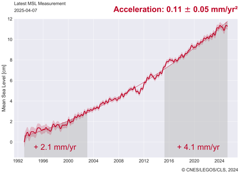
The notion that anyone who is making as basic a mathematical point as acceleration being defined by the second time-derivate of displacement (i.e., by the time derivative of velocity) needs to SHOW THEIR WORK betrays a stupendous lack of analytic comprehension (see: https://en.wikipedia.org/wiki/Acceleration).
For those interested in demonstrating to themselves that there was considerable acceleration evident in satellite data after 2011, I would recommend simply running the discrete ROC estimator [f(n+1) – f(n-1)] / 2 through the data recursively, always centering the result at t = n. That sporadic acceleration, along with the current deceleration, will show up unmistakably upon applying any reasonable smoothing, before or after using the estimator.
1sky1, it appears that you still have missed my comment from five days ago, wherein I said:
Regards,
w.
Fix your own fundamental mistakes, instead of imposing upon others.
To be more precise, successive (cascade) application of the estimator is here loosely termed “recursively.”