Guest essay by George White
For matter that’s absorbing and emitting energy, the emissions consequential to its temperature can be calculated exactly using the Stefan-Boltzmann Law,
1) P = εσT4
where P is the emissions in W/m2, T is the temperature of the emitting matter in degrees Kelvin, σ is the Stefan-Boltzmann constant whose value is about 5.67E-8 W/m2 per K4 and ε is the emissivity which is 1 for an ideal black body radiator and somewhere between 0 and 1 for a non ideal system also called a gray body. Wikipedia defines a Stefan-Boltzmann gray body as one “that does not absorb all incident radiation” although it doesn’t specify what happens to the unabsorbed energy which must either be reflected, passed through or do work other than heating the matter. This is a myopic view since the Stefan-Boltzmann Law is equally valid for quantifying a generalized gray body radiator whose source temperature is T and whose emissions are attenuated by an equivalent emissivity.
To conceptualize a gray body radiator, refer to Figure 1 which shows an ideal black body radiator whose emissions pass through a gray body filter where the emissions of the system are observed at the output of the filter. If T is the temperature of the black body, it’s also the temperature of the input to the gray body, thus Equation 1 still applies per Wikipedia’s over-constrained definition of a gray body. The emissivity then becomes the ratio between the energy flux on either side of the gray body filter. To be consistent with the Wikipedia definition, the path of the energy not being absorbed is omitted.

A key result is that for a system of radiating matter whose sole source of energy is that stored as its temperature, the only possible way to affect the relationship between its temperature and emissions is by varying ε since the exponent in T4 and σ are properties of immutable first principles physics and ε is the only free variable.
The units of emissions are Watt/meter2 and one Watt is one Joule per second. The climate system is linear to Joules meaning that if 1 Joule of photons arrives, 1 Joule of photons must leave and that each Joule of input contributes equally to the work done to sustain the average temperature independent of the frequency of the photons carrying that energy. This property of superposition in the energy domain is an important, unavoidable consequence of Conservation of Energy and often ignored.
The steady state condition for matter that’s both absorbing and emitting energy is that it must be receiving enough input energy to offset the emissions consequential to its temperature. If more arrives than is emitted, the temperature increases until the two are in balance. If less arrives, the temperature decreases until the input and output are again balanced. If the input goes to zero, T will decay to zero.
Since 1 calorie (4.18 Joules) increases the temperature of 1 gram of water by 1C, temperature is a linear metric of stored energy, however; owing to the T4 dependence of emissions, it’s a very non linear metric of radiated energy so while each degree of warmth requires the same incremental amount of stored energy, it requires an exponentially increasing incoming energy flux to keep from cooling.
The equilibrium climate sensitivity factor (hereafter called the sensitivity) is defined by the IPCC as the long term incremental increase in T given a 1 W/m2 increase in input, where incremental input is called forcing. This can be calculated for emitting matter in LTE by differentiating the Stefan-Boltzmann Law with respect to T and inverting the result. The value of dT/dP has the required units of degrees K per W/m2 and is the slope of the Stefan-Boltzmann relationship as a function of temperature given as,
2) dT/dP = (4εσT3)-1
A black body is nearly an exact model for the Moon. If P is the average energy flux density received from the Sun after reflection, the average temperature, T, and the sensitivity, dT/dP can be calculated exactly. If regions of the surface are analyzed independently, the average T and sensitivity for each region can be precisely determined. Due to the non linearity, it’s incorrect to sum up and average all the T’s for each region of the surface, but the power emitted by each region can be summed, averaged and converted into an equivalent average temperature by applying the Stefan-Boltzmann Law in reverse. Knowing the heat capacity per m2 of the surface, the dynamic response of the surface to the rising and setting Sun can also be calculated all of which was confirmed by equipment delivered to the Moon decades ago and more recently by the Lunar Reconnaissance Orbiter. Since the lunar surface in equilibrium with the Sun emits 1 W/m2 of emissions per W/m2 of power it receives, its surface power gain is 1.0. In an analytical sense, the surface power gain and surface sensitivity quantify the same thing, except for the units, where the power gain is dimensionless and independent of temperature, while the sensitivity as defined by the IPCC has a T-3 dependency and which is incorrectly considered to be approximately temperature independent.
A gray body emitter is one where the power emitted is less than would be expected for a black body at the same temperature. This is the only possibility since the emissivity can’t be greater than 1 without a source of power beyond the energy stored by the heated matter. The only place for the thermal energy to go, if not emitted, is back to the source and it’s this return of energy that manifests a temperature greater than the observable emissions suggest. The attenuation in output emissions may be spectrally uniform, spectrally specific or a combination of both and the equivalent emissivity is a scalar coefficient that embodies all possible attenuation components. Figure 2 illustrates how this is applied to Earth, where A represents the fraction of surface emissions absorbed by the atmosphere, (1 – A) is the fraction that passes through and the geometrical considerations for the difference between the area across which power is received by the atmosphere and the area across which power is emitted are accounted for. This leads to an emissivity for the gray body atmosphere of A and an effective emissivity for the system of (1 – A/2).

The average temperature of the Earth’s emitting surface at the bottom of the atmosphere is about 287K, has an emissivity very close to 1 and emits about 385 W/m2 per Equation 1. After accounting for reflection by the surface and clouds, the Earth receives about 240 W/m2 from the Sun, thus each W/m2 of input contributes equally to produce 1.6 W/m2 of surface emissions for a surface power gain of 1.6.
Two influences turn 240 W/m2 of solar input into 385 W/m2 of surface output. First is the effect of GHG’s which provides spectrally specific attenuation and second is the effect of the water in clouds which provides spectrally uniform attenuation. Both warm the surface by absorbing some fraction of surface emissions and after some delay, recycling about half of the energy back to the surface. Clouds also manifest a conditional cooling effect by increasing reflection unless the surface is covered in ice and snow when increasing clouds have only a warming influence.
Consider that if 290 W/m2 of the 385 W/m2 emitted by the surface is absorbed by atmospheric GHG’s and clouds (A ~ 0.75), the remaining 95 W/m2 passes directly into space. Atmospheric GHG’s and clouds absorb energy from the surface, while geometric considerations require the atmosphere to emit energy out to space and back to the surface in roughly equal proportions. Half of 290 W/m2 is 145 W/m2 which when added to the 95 W/m2 passed through the atmosphere exactly offsets the 240 W/m2 arriving from the Sun. When the remaining 145 W/m2 is added to the 240 W/m2 coming from the Sun, the total is 385 W/m2 exactly offsetting the 385 W/m2 emitted by the surface. If the atmosphere absorbed more than 290 W/m2, more than half of the absorbed energy would need to exit to space while less than half will be returned to the surface. If the atmosphere absorbed less, more than half must be returned to the surface and less would be sent into space. Given the geometric considerations of a gray body atmosphere and the measured effective emissivity of the system, the testable average fraction of surface emissions absorbed, A, can be predicted as,
3) A = 2(1 – ε)
Non radiant energy entering and leaving the atmosphere is not explicitly accounted for by the analysis, nor should it be, since only radiant energy transported by photons is relevant to the radiant balance and the corresponding sensitivity. Energy transported by matter includes convection and latent heat where the matter transporting energy can only be returned to the surface, primarily by weather. Whatever influences these have on the system are already accounted for by the LTE surface temperatures, thus their associated energies have a zero sum influence on the surface radiant emissions corresponding to its average temperature. Trenberth’s energy balance lumps the return of non radiant energy as part of the ‘back radiation’ term, which is technically incorrect since energy transported by matter is not radiation. To the extent that latent heat energy entering the atmosphere is radiated by clouds, less of the surface emissions absorbed by clouds must be emitted for balance. In LTE, clouds are both absorbing and emitting energy in equal amounts, thus any latent heat emitted into space is transient and will be offset by more surface energy being absorbed by atmospheric water.
The Earth can be accurately modeled as a black body surface with a gray body atmosphere, whose combination is a gray body emitter whose temperature is that of the surface and whose emissions are that of the planet. To complete the model, the required emissivity is about 0.62 which is the reciprocal of the surface power gain of 1.6 discussed earlier. Note that both values are dimensionless ratios with units of W/m2 per W/m2. Figure 3 demonstrates the predictive power of the simplest gray body model of the planet relative to satellite data.
Figure 3

Each little red dot is the average monthly emissions of the planet plotted against the average monthly surface temperature for each 2.5 degree slice of latitude. The larger dots are the averages for each slice across 3 decades of measurements. The data comes from the ISCCP cloud data set provided by GISS, although the output power had to be reconstructed from radiative transfer model driven by surface and cloud temperatures, cloud opacity and GHG concentrations, all of which were supplied variables. The green line is the Stefan-Boltzmann gray body model with an emissivity of 0.62 plotted to the same scale as the data. Even when compared against short term monthly averages, the data closely corresponds to the model. An even closer match to the data arises when the minor second order dependencies of the emissivity on temperature are accounted for,. The biggest of these is a small decrease in emissivity as temperatures increase above about 273K (0C). This is the result of water vapor becoming important and the lack of surface ice above 0C. Modifying the effective emissivity is exactly what changing CO2 concentrations would do, except to a much lesser extent, and the 3.7 W/m2 of forcing said to arise from doubling CO2 is the solar forcing equivalent to a slight decrease in emissivity keeping solar forcing constant.
Near the equator, the emissivity increases with temperature in one hemisphere with an offsetting decrease in the other. The origin of this is uncertain but it may be an anomaly that has to do with the normalization applied to use 1 AU solar data which can also explain some other minor anomalous differences seen between hemispheres in the ISCCP data, but that otherwise average out globally.
When calculating sensitivities using Equation 2, the result for the gray body model of the Earth is about 0.3K per W/m2 while that for an ideal black body (ε = 1) at the surface temperature would be about 0.19K per W/m2, both of which are illustrated in Figure 3. Modeling the planet as an ideal black body emitting 240 W/m2 results in an equivalent temperature of 255K and a sensitivity of about 0.27K per W/m2 which is the slope of the black curve and slightly less than the equivalent gray body sensitivity represented as a green line on the black curve.
This establishes theoretical possibilities for the planet’s sensitivity somewhere between 0.19K and 0.3K per W/m2 for a thermodynamic model of the planet that conforms to the requirements of the Stefan-Boltzmann Law. It’s important to recognize that the Stefan-Boltzmann Law is an uncontroversial and immutable law of physics, derivable from first principles, quantifies how matter emits energy, has been settled science for more than a century and has been experimentally validated innumerable times.
A problem arises with the stated sensitivity of 0.8C +/- 0.4C per W/m2, where even the so called high confidence lower limit of 0.4C per W/m2 is larger than any of the theoretical values. Figure 3 shows this as a blue line drawn to the same scale as the measured (red dots) and modeled (green line) data.
One rationalization arises by inferring a sensitivity from measurements of adjusted and homogenized surface temperature data, extrapolating a linear trend and considering that all change has been due to CO2 emissions. It’s clear that the temperature has increased since the end of the Little Ice Age, which coincidently was concurrent with increasing CO2 arising from the Industrial Revolution, and that this warming has been a little more than 1 degree C, for an average rate of about 0.5C per century. Much of this increase happened prior to the beginning the 20’th century and since then, the temperature has been fluctuating up and down and as recently as the 1970’s, many considered global cooling to be an imminent threat. Since the start of the 21’st century, the average temperature of the planet has remaining relatively constant, except for short term variability due to natural cycles like the PDO.
A serious problem is the assumption that all change is due to CO2 emissions when the ice core records show that change of this magnitude is quite normal and was so long before man harnessed fire when humanities primary influences on atmospheric CO2 was to breath and to decompose. The hypothesis that CO2 drives temperature arose as a knee jerk reaction to the Vostok ice cores which indicated a correlation between temperature and CO2 levels. While such a correlation is undeniable, newer, higher resolution data from the DomeC cores confirms an earlier temporal analysis of the Vostok data that showed how CO2 concentrations follow temperature changes by centuries and not the other way around as initially presumed. The most likely hypothesis explaining centuries of delay is biology where as the biosphere slowly adapts to warmer (colder) temperatures as more (less) land is suitable for biomass and the steady state CO2 concentrations will need to be more (less) in order to support a larger (smaller) biomass. The response is slow because it takes a while for natural sources of CO2 to arise and be accumulated by the biosphere. The variability of CO2 in the ice cores is really just a proxy for the size of the global biomass which happens to be temperature dependent.
The IPCC asserts that doubling CO2 is equivalent to 3.7 W/m2 of incremental, post albedo solar power and will result in a surface temperature increase of 3C based on a sensitivity of 0.8C per W/m2. An inconsistency arises because if the surface temperature increases by 3C, its emissions increase by more than 16 W/m2 so 3.7 W/m2 must be amplified by more than a factor of 4, rather than the factor of 1.6 measured for solar forcing. The explanation put forth is that the gain of 1.6 (equivalent to a sensitivity of about 0.3C per W/m2) is before feedback and that positive feedback amplifies this up to about 4.3 (0.8C per W/m2). This makes no sense whatsoever since the measured value of 1.6 W/m2 of surface emissions per W/m2 of solar input is a long term average and must already account for the net effects from all feedback like effects, positive, negative, known and unknown.
Another of the many problems with the feedback hypothesis is that the mapping to the feedback model used by climate science does not conform to two important assumptions that are crucial to Bode’s linear feedback amplifier analysis referenced to support the model. First is that the input and output must be linearly related to each other, while the forcing power input and temperature change output of the climate feedback model are not owing to the T4 relationship between the required input flux and temperature. The second is that Bode’s feedback model assumes an internal and infinite source of Joules powers the gain. The presumption that the Sun is this source is incorrect for if it was, the output power could never exceed the power supply and the surface power gain will never be more than 1 W/m2 of output per W/m2 of input which would limit the sensitivity to be less than 0.2C per W/m2.
Finally, much of the support for a high sensitivity comes from models. But as has been shown here, a simple gray body model predicts a much lower sensitivity and is based on nothing but the assumption that first principles physics must apply, moreover; there are no tuneable coefficients yet this model matches measurements far better than any other. The complex General Circulation Models used to predict weather are the foundation for models used to predict climate change. They do have physics within them, but also have many buried assumptions, knobs and dials that can be used to curve fit the model to arbitrary behavior. The knobs and dials are tweaked to match some short term trend, assuming it’s the result of CO2 emissions, and then extrapolated based on continuing a linear trend. The problem is that there as so many degrees of freedom in the model, it can be tuned to fit anything while remaining horribly deficient at both hindcasting and forecasting.
The results of this analysis explains the source of climate science skepticism, which is that IPCC driven climate science has no answer to the following question:
What law(s) of physics can explain how to override the requirements of the Stefan-Boltzmann Law as it applies to the sensitivity of matter absorbing and emitting energy, while also explaining why the data shows a nearly exact conformance to this law?
References
1) IPCC reports, definition of forcing, AR5, figure 8.1, AR5 Glossary, ‘climate sensitivity parameter’
2) Kevin E. Trenberth, John T. Fasullo, and Jeffrey Kiehl, 2009: Earth’s Global Energy Budget. Bull. Amer. Meteor. Soc., 90, 311–323.
3) Bode H, Network Analysis and Feedback Amplifier Design assumption of external power supply and linearity: first 2 paragraphs of the book
4) Manfred Mudelsee, The phase relations among atmospheric CO content, temperature and global ice volume over the past 420 ka, Quaternary Science Reviews 20 (2001) 583-589
5) Jouzel, J., et al. 2007: EPICA Dome C Ice Core 800KYr Deuterium Data and Temperature Estimates.
6) ISCCP Cloud Data Products: Rossow, W.B., and Schiffer, R.A., 1999: Advances in Understanding Clouds from ISCCP. Bull. Amer. Meteor. Soc., 80, 2261-2288.
7) “Diviner Lunar radiometer Experiment” UCLA, August, 2009
Frank
The lapse rate is NOT set by convection.
It is set by gravity sorting molecules into a density gradient such that the gas laws dictate a lower temperature for a lower density. Therefore, however much conduction occurs at the surface there will always be a lapse rate and an isothermal atmosphere cannot arise even with no GHGs at all.
Convection is a consequence of the lapse rate when uneven heating occurs via conduction (a non radiative process) at the surface beneath. The uneven surface warmimg makes parcels of gas in contact with the surface lighter than adjoining parcels so that they rise upward adiabatically in an attempt to match the density of the warmer parcel with the density of the colder air higher up..No radiative gases required.
Convective overturning is a zero sum closed loop as far as the adiabatic component (most of it in our largely non radiative atmosphere) is concerned.
Radiative imbalances are neutralised by convective adjustments within an atmosphere in hydrostatic equilibrium.
http://www.public.asu.edu/~hhuang38/mae578_lecture_06.pdf
“Radiative equilibrium
profile could be unstable;
convection restores it
to stability (or neutrality)”
George,
I don’t know why you’re invoking DLR at the surface as some sort of means of explaining your derived equivalent model. It’s causing massive confusion and misunderstanding (see Frank’s latest post). To me, the entire point the model is ultimately making is DLR at the surface has no clear connection to A’s aggregate ability to ultimately drive and manifest enhanced surface warming, i.e. no clear connection to the underlying driving physics of the GHE via the absorption and (non-directional) re-radiation of surface emitted IR by GHGs amongst all the other effects, radiant and non-radiant, known and unknown, that are manifesting the energy balance.
I’m perplexed why you think Ps*A/2 is attempting saying anything about DLR at the surface. To me, the whole point is it’s not. It’s instead quantifying something else entirely.
Let’s be clear that what I (and I presume Frank) are referring to by DLR at the surface is the total amount of IR flux emitted from the atmosphere (as a whole mass) that *passes* to and is absorbed by the surface. Not saying it’s all necessarily added to the net flux gained the surface. Is this clear?
You’ve kind of lost me a little here with these last few posts of yours.
And that only about half of ‘A’ ultimately contributes to the overall downward IR push made in the atmosphere that drives and ultimately leads to enhanced surface warming (via the GHE). The point being it’s the downward IR push within or the divergence of upwelling surface IR captured and re-emitted back towards (and not necessarily back to the surface) that is the fundamental underlying driving mechanism slowing down the upward IR cooling that ultimately leads to enhanced warming of the surface — not DLR at the surface.
If this is not correct, then I don’t understand your model (as I thought I did).
RW,
Your description of how absorbed energy per A is redistributed is correct.
OK, I’m relieved.
Your atmospheric RT simulator must calculate and have a value for downward IR intensity at the surface. I recall you’ve said its about 300 W/m^2 (or maybe 290 W/m^2 or something).
I don’t know why you’re going the route of surface DLR to explain your model. It seems to be causing massive confusion on an epic scale.
George,
As clearly evidenced by this post here:
https://wattsupwiththat.com/2017/01/05/physical-constraints-on-the-climate-sensitivity/comment-page-1/#comment-2395000
Frank has absolutely no clue what you’re doing here with this whole thing. He’s totally and completely faked out.
There’s got be a better way to step everyone through what you’re doing here with this exercise and derived equivalent model. I know it’s second nature to you what you’re doing with all of this (since you’ve successfully applied these techniques to a zillion different systems over the years), but most everyone else has no clue from what foundation all of this is coming from. They think this is spectacular nonsense, and it surely would be if what you’re actually doing and claiming with it is what they think it is.
Many do not seem to grasp that the purpose of this model was to model the sensitivity and validate the model with data representing what was being modeled, which is the photon flux at the top and bottom boundaries of the atmosphere, where the photon flux at the bottom is related to the temperature we care about. If the boundaries can be modeled, it doesn’t matter how they got that way, just that they do and that we can quantify the sensitivity relative to the transfer function quantifying the relationship between those boundaries.
Some fail to grasp the purpose because they deny the consequences. Others are bamboozled by excess complexity, others don’t understand the difference between photons and molecules in motion and still others are misdirected by their own specific idea of how things work. For example some think that the lapse rate sets the surface temperature. Nothing could be further from the truth since the lapse RATE is independent of the surface temperature, moreover; the atmospheric temperature profile is only linear to a lapse rate for a small fraction of its height.
BTW, my responses going forward will be fewer and farther between since I intend to get some serious skiing in over the next few months. I finally got to Tahoe, Squaw has been closed for days and the top has as much as 15′ of fresh powder.
George,
“Many do not seem to grasp that the purpose of this model was to model the sensitivity and validate the model with data representing what was being modeled, which is the photon flux at the top and bottom boundaries of the atmosphere, where the photon flux at the bottom is related to the temperature we care about. If the boundaries can be modeled, it doesn’t matter how they got that way, just that they do and that we can quantify the sensitivity relative to the transfer function quantifying the relationship between those boundaries.”
I understand all of this, but others like Frank clearly don’t and are totally faked out. He has no clue what you’re doing with all of this.
For one, you need to make it clear that your derived equivalent model only accounts for EM radiation, because the entire energy budget is all EM radiation, EM radiation is all that can pass across the system’s boundary between the atmosphere and space, and the surface emits EM radiation back up into the atmosphere at the same rate its gaining joules as a result of all the physical processes in the system, radiant and non-radiant, known and unknown. This is why your model doesn’t include or quantify non-radiant fluxes.
They fundamentally don’t understand that your model is just the simplest construct that gives the same average behavior, i.e the same rates of joules gained and lost at the surface and TOA, while fully conserving all joules, radiant and non-radiant, being moved around to physically manifest it. And that the model is *only* a quantification of aggregate, already physically manifested, behavior. Or only a quantification of the aggregate behavior of the complex, high non-linear thermodynamic path manifesting the energy balance. They think your model is trying to model or emulate the actual thermodynamics and thermodynamic path manifesting the energy balance, as evidenced by Frank’s latest post.
“Validate” is the wrong word. One cannot “validate” a model absent the underlying statistical population. “Evaluate” is the IPCC-blessed word for the cockeyed way in which global warming models are tested.
Terry,
OK. How about attempting to falsify my hypothesis which didn’t fail.
BTW, I think I have and adequate sample space. I’m not attempting to identify trends from a time series, but using each of millions of individual measurements spanning all possible conditions found on the planet as representative of the transfer function quantifying the relationship between the radiant emissions of the surface consequential to its temperature and the emissions of the planet.
co2:
Contrary to how the phrase sounds, the “sample space” is not the entity from which a sample is drawn. Instead it is the “sampling frame” from which a sample is drawn. The “sample space” is the complete set of the possible outcomes of events.
The elements of the sampling frame are the “sampling units.” The complete set of sampling units is the “statistical population.” For global warming climatology there is no statistical population or sampling frame. There are no sampling units. Thus there are no samples.There are, however, a number of different temperature time series. Many bloggers confuse a temperature time series with a statistical population thus reaching the conclusion that a model can be validated when it cannot. To attempt scientific research absent the statistical population is the worst blunder that a researcher can make as it assures that the resulting model will generate no information.
I agree with you, but you can’t just try finding statistical significance between different measured values thinking that will give you insight.
And too much of this seems, like is what is going on, lot of computing power available in most pc’s to do all sorts of things with statistics. But you won’t find it until you know the topic well enough to spot the areas that have seams, and roughness spots that need examined, and then you have to keep digging until you figure it out.
Terry,
“:Many bloggers confuse a temperature time series with a statistical population thus reaching the conclusion that a model can be validated when it cannot. ”
Yes, when trying to predict the future based on a short time series of the past. There’s just too much long to medium term periodicity of unknown origin to extrapolate a linear trend from a short term time series.
My point is that I have millions of samples of behavior from more than a dozen different satellites covering all possible surface and atmospheric condition whose average response is most definitely statistically significant. Not to extrapolate a trend, but to quantify the response to change,
Terry, your attempt at obscuring the definitions of things makes you look ridiculous. A specific element in any given time series is an n-tuple of a) geographical coordinates, b) date/time stamp and c) a measured value. The “sample space is the set of ALL n-tuples. An element of a time series is called a sample drawn from the above mentioned sample space. Your use of the word “frame” is not applicable to what co2isnotevil is talking about. If you wish to introduce new terms to this discussion, please define them rigorously, or don’t use them.
The whole point here, if I’m understanding this all correctly, is the radiative physics of the GHE that ultimately leads to enhanced surface warming are *applied* physics within the physics of atmospheric radiative transfer. The physics of atmospheric radiative transfer are NOT by themselves the physics of the GHE, or more specifically NOT the underlying driving physics of the GHE. This is a somewhat subtle, but crucial fundamental point relative to what you’re doing and modeling here that needs to be grasped and understood by everyone from the outset.
DLR at the surface is the ultimate manifestation of the downward IR intensity through the whole of the atmosphere predicted by the Schartzchild eqn. at the surface/atmosphere boundary. This physical manifestation, however, is not the underlying physics of the GHE (or more specifically the underlying physics driving the GHE). Moreover perhaps, its manifestation at the surface has no clear relationship to absorptance A’s ability to drive the ultimate manifestation of enhanced surface warming, i.e. greenhouse warming of the surface via the absorption of surface IR by GHGs and the subsequent (non-directional) re-radiation of that absorbed surface IR energy among all of the other effects that manifest the energy balance (radiant and non-radiant).
RW, and you can see the applied physics in this
I’ll be on vacation and out of touch until Monday, Jan 16. Please defer responses until then.
co2isnotevil said:
“The surface of the planet only emits a NET of 385 W/m^2 consequential to its temperature. Latent heat and thermals are not emitted, but represents a zero sum from an energy perspective since any effect the round trip path that energy takes has is already accounted for by the average surface temperature. The surface requires 385 W/m^2 of input to offset the 385 W/m^2 being emitted. ”
This is a point I made here some time ago about the Trnberth energy budget which shows latent heat and thermals going up but not returning to the surface in a zero sum adiabatic/convective loop.
Instead Trenberth racked up DWIR to the surface by an identical amount and I pointed that out as a mistake.
Many didn’t get it then and are not getting it now.
George’s work, if correctly interpreted, shows that any DWIR from the atmosphere is already included in the S-B surface temperature with no additional surface temperature enhancement necessary or required. The reason being that at S-B surface temperature (beneath an atmosphere) WITH NO NON RADIATIVE PROCESSES GOING ON radiation to space from within the atmosphere would be matched by a reduction of radiation to space from the surface for a zero net effect.
If one then adds convection as a non radiative process and acknowledge that convection up and down requires a separate closed energy loop then it follows that the surface temperature rises above S-B as a result of the non radiative processes alone
George’s work appears to validate that since to get emission to space at 255k one needs a surface temperature of 33K higher than S-B to accommodate the additional surface energy tied up in non radiative processes.
Trenberth et al have failed to account for the return of non radiative energy towards the surface via the PE to KE exchange in descending air.
I don’t think your assessment of George’s work is correct. He agrees that added GHGs will enhance the GHE and ultimately lead to some surface warming (to restore balance at the TOA). He’s disputing the magnitude of surface warming that will occur.
RW,
I think George hasn’t yet realised the implications of his work. Maybe he will comment himself shortly. I suggested higher up the thread that for added GHGs to enhance the GHE it would have to cause the red curve to fail to follow the green curve but he seems to be saying that doesn’t happen.
I’m pretty sure (I don’t want to put words in his mouth) he is, very similar to what Anthony and Willis just published, and it’s the TOA view of what I’ve found looking up.
What is shows is the surface temp follows water vapor, and water vapor is so ubiquitous it’s affect completely (>90%) overwhelms the ghg effect of co2 on temperature.
In this case George has shown this effect looks identical to an e=.62.
micro6500
Water vapour certainly does make it far easier for the necessary convective adjustments to be made so as to neutralise the effect of non condensing GHGs such as CO2. The phase changes are very powerful.
Water vapour causes the lapse rate slope to skew to the warm side so it is less steep. A less steep lapse rate slope slows down convection which allows humidity to rise. When humidity rises the dew point changes so that the vapour can condense out at a lower warmer height which then causes more radiation to space from clouds at the lower warmer height.
That offsets the potential warming effect of CO2 and that is the mechanism which I suggested to David Evans when he was developing his hypothesis about multiple variable ‘pipes’ for radiative loss to space. The water vapour pipe increases to compensate for any reduction in the GHG (or CO2) pipe.
But in the end, even without water vapour, convection would neutralise the radiative imbalance derived from non condensing GHGs and even if it does not do so the effect of GHGs is reduced to near zero anyway because the main cause of the GHE is convection within atmospheric mass as explained above.
“When humidity rises the dew point changes” only if the air mass carries additional water in, but the conditions I’ve been discussing that is not part of the process, absolute humidity changes slowly as fronts move in. Rel humidity swings with temp, so changes significantly over a day, regardless of a weather change.
To be absolutely clear, I do not dispute the fact that GHG’s and clouds warm the surface beyond what it would be without them and that both influences are purely radiative. But again, demonstrating this either way is not the purpose of this analysis which was focused on the sensitivity.
The purpose was to separate the radiation out, model how it should behave by extracting the transfer function between surface temperature and planet emissions, test the resulting model with data measuring what is being predicted and if the model correctly describes the relationship between the surface temperature to the planets emissions into space, it also must quantify the sensitivity, which the IPCC defines as the incremental relationship between these two factors. This whole exercise is nothing more than an application of the scientific method to ascertain a quantitative measure of the sensitivity which to date has never been done.
My original hypothesis was that the radiation fluxes MUST obey physical laws at the boundaries of the atmosphere and the best candidate for a law to follow was SB. The reason is that without an atmosphere, the planet is perfectly quantified as a BB (neglecting reflection as ‘grayness’) and the only way to modify this behavior is with a non unit emissivity, which the atmosphere provides, relative to the surface. This is the only possible way to ‘connect the dots’ between BB behavior and the observed behavior.
Subsequent to this, I began to understand why this must be the case which is that a system with sufficient degrees of freedom will self organize itself towards ideal behavior as the goal of minimizing changes in entropy. If you look here under ‘Demonstrations of Control’, I’m considering writing another piece explaining how these plots arise as consequence of this hypothesis.
http://www.palisad/com/co2/sens
co2isnotevil said this:
“I do not dispute the fact that GHG’s and clouds warm the surface beyond what it would be without them and that both influences are purely radiative”
Well, if you have radiative material within an atmosphere which is radiating out to space but not radiating to the surface then the surface would cool below S-B.
But if that radiative material is also radiating down to the surface then the surface will indeed be warmed beyond what it otherwise would be but not to beyond the S-B expectation, only up to it.
So, do GHGs radiate out to space at a different rate to the rate at which they radiate down to the surface or not ?
The atmosphere is indefinitely maintained in hydrostatic equilibrium with no net radiative imbalances overall and so the balance MUST be equal once hydrostatic equilibrium has been attained.
For CO2 molecules the idea is that they block outgoing at a certain wavelength so presumably they are supposed to radiate downward more powerfully than they radiate to space.
Yet George shows that for the system as a whole the surface temperature curve follows the S-B curve in his diagram and he concludes that the system always moves successfully back to the ‘ideal’.
That being the case, how can one reserve a residual RADIATIVE surface warming effect beyond S-B for any component of the atmosphere?
I suggest that in so far as CO2 blocks outgoing radiation the water vapour ‘pipe’ counters any potential warming effect and even if there were no water vapour then other radiative material within the atmosphere operates to the same effect just as well. For example, stronger winds would kick up more dust which is radiative material and convection would ensure that radiation from such material would go out to space from the correct height along the lapse rate slope to ensure maintenance of hydrostatic equilibrium.
Mars is a good example. I aver that the planet wide dust storms on Mars arise when the surface temperature rises too high for hydrostatic equilibrium so that winds increase, dust is kicked up and radiation to space from that dust increases until equilibrium is restored.
Only a NON RADIATIVE surface warming effect fits the bill in every respect and that is identifiable not in the similarity between the slopes of the red and green curves but rather in the distance between the red and green curves.
Water is the current main working fluid, where our planet is about in the middle of it’s 3 states temperature.


But this is the actual net surface radiation with temp and rel humidity. This is 5 days, mostly clear, a few cumulus clouds on the middle two days afternoon.
Then zoomed in so you can see the net outgoing radiation
When this is going on at night, the switching between water open and water closed, it is visibly clear out. So as air temps near dew points, the water window closes to ir (but not visible), and the outgoing clear calm skies drops by about 2/3rds. This is where the e=.62 comes from.
The temp globally does this.
Co2 is ineffective at affecting temps, at least with all of the water vapor.
Co2 does impact both rates by the 2 whatever watts, but some rel humidity is a temperature effect, it will stay in the high rate longer, until any excess temperature energy in the surface system (in relationship to dew point) is radiated away, the net rad measurement shows this. It does all of this with no measurable convection. Maybe 1,000 feet, but dead calm at the surface, and the first graph explains what surface temps are doing.
Notice that there is almost no measured increase in max temperature? only min. And when you look at min alone, it jumps with dew point during the 97 El Nino, that is all that has happened, the oceans changed where the water vapor went.
micro6500,
I consider water to be the refrigerant in a heat pump implementing what we call weather. Follow the water and its a classic Carnot cycle.
It’s certainly true that Co2 is a far less effective GHG than water vapor, moreover; water vapor is dynamic and provides the raw materials for the radiative balance control system. The volume of clouds is roughly proportional to atmospheric water content, but the ratio between cloud height and cloud area is one of those degrees of freedom I mentioned that drives the system towards an idealized steady state consistent with it’s goal to minimize changes in entropy in response to perturbations to the system or its stimulus.
Then you are not understanding the chart I keep showing. What it’s showing is a temperature regulated switch that turns off 70% or so of the outgoing radiation from the surface once the set temp is reached. The set point temperature follows humidity levels.
This process regulates morning minimum temperature everywhere rel humidity reaches 100% at night under clear calm skies.
Yes, but you can’t directly measure that in your own backyard to whatever suitable accuracy to satisfy that co2 is not doing anything. I mean really glad you did this, it’s been needed for a long time. But it doesn’t kill their argument.
Actually a test, I think you would say e will change as ghg increase forcing, at 62% or so. If what I discovered works like I think it will be more like less than 5 or 10%.
And I think if you look at the temp record, you’d see it can’t be 62%.
“So, do GHGs radiate out to space at a different rate to the rate at which they radiate down to the surface or not ?”
If geometry matters, its equal.
Stephen,
“So, do GHGs radiate out to space at a different rate to the rate at which they radiate down to the surface or not ?”
I would say, yes they do; however, this is a function of emission rate decreasing with height and NOT because the probability of photon emitted within is greater downwards than upwards. This is a key distinction that relates to all of this that many seem to be missing. With regard to what George is quantifying as ‘A’, the re-emission of ‘A’ is by and large equal in any direction regardless of the emitting rate where any portion of ‘A’ is actually absorbed. Even clouds are made up of small droplets that themselves radiate (individually) roughly equally in all directions, though of course the top of the clouds generally emit less IR up than the bottom of clouds emit IR downward.
RW, I would go with George on this. Although temperature declines with height and the emission rate declines accordingly a cloud at any given height will radiate equally in all directions based on its temperature at that height.
The depth of the cloud would be dealt with in the average emissions from the entire cloud.
Micro6500
Your graphs relate to emissions from the surface but I was considering emissions from clouds to space. At a lower height along the lapse rate slope a cloud is warmer and radiates more to space. CO2 causes the cloud heights to drop. That is a mechanism whereby the ‘blocking’ of radiation to space by CO2 can be neutralised.
Maybe it can, but it does not interfere with the decaying rate of cooling under clear skies that I have discovered that is from 2 cooling rates controlled by water vapor. The global average of min temp following dew points shows it is a global mechanism.
How is that relevant to the point I made?
Because I don’t think the two are associated, I don’t see how cloud top emissions can counter how wv closes the path for a significant amount of energy to space under clear skies. So, maybe I misunderstood your comment relating to this clear sky effect.
I didn’t say that cloud top emissions counter how water vapour closes such a path. I was referring to the outgoing wavelengths blocked by CO2.
CO2 absorbs those wavelenghs and prevents their emission to space. That distorts the lapse rate to the warm side, the rate of convection drops, humidity builds up at lower levels and clouds form at a lower warmer height because greater humidity causes clouds to form at a higher temperature and lower height for example 100% humidity allows fog to condense out at surface ambient temperature.
I think this is ~33% mixture, and it doesn’t completely block 15u. Now, I can be pedantic, so if that’s all it is, okay, sorry 🙂
http://webbook.nist.gov/cgi/cbook.cgi?ID=C124389&Units=SI&Type=IR-SPEC&Index=1#IR-SPEC
Stole this from Frank
Exactly.
The diffraction at the surface is because the speed of light in the material changes compared to a vacuum, or the medium those photons come from (ie different types of glass used in a pair of lens that are physically in contact with each other). The reason it’s a different speed is the atoms interact with that wavelength of photon, but it can still be transparent, like glass.
Maybe these help explain my thoughts on this.
Micro,
I see that I made a typo which has misled you. Sorry.
I typed ‘water vapour’ instead of ‘CO2’ in my post at 9.40 am.
It is the distortion of the lapse rate by CO2 that I was intending to talk about.
micro6500 January 13, 2017 at 6:54 am
“CO2 absorbs those wavelenghs and prevents their emission to space.”
I think this is ~33% mixture, and it doesn’t completely block 15u. Now, I can be pedantic, so if that’s all it is, okay, sorry 🙂
http://webbook.nist.gov/cgi/cbook.cgi?ID=C124389&Units=SI&Type=IR-SPEC&Index=1#IR-SPEC
And a path length of only 10 cm.
A high res spectra under those conditions shows complete absorption in the Q-branch but of course our atmosphere is a lot thicker than 10cm. At 400ppm the atmosphere will show a similar high res spectra at 10m.
All true, but not blocked to space? Right?
And Phil, I’d like your thoughts on this if you can take a look.
https://micro6500blog.wordpress.com/2016/12/01/observational-evidence-for-a-nonlinear-night-time-cooling-mechanism/
Since we’ve talked a lot of this sort of thing.
“However, if an object doesn’t emit at some wavelength, then it doesn’t absorb at that wavelength either and it is semi-transparent.”
This is inconsistent with Planck law which demonstrates any massive object with positive radii and diameter much larger than wavelength of interest (semi-transparent or opaque) emits at all wavelengths at all temperatures, and a given angle of incidence and polarization, emissivity = absorptivity.
Plancks Law is more relevant to liquids and solids. Gases emit and absorb specific wavelengths and its really not until it’s heated into a plasma that it will emit radiation conforming to Plancks Law. O2/N2 at 1 ATM neither absorbs or emits any measurable amount of radiation in the LWIR spectrum that the Earth emits. i.e. emissivity = absorption = 0
“..its really not until it’s heated into a plasma that it will emit radiation conforming to Plancks Law.”
Not correct, gases radiate according to Planck law at all temperatures, all wavelengths including N2 and O2. Emissivity over the spectrum, in a hemisphere of directions would be very low for N2/O2 atm. but nonzero as shown by Planck law & measured gas emissivity over the spectrum.
Envisage a radiative atmosphere in hydrostatic equilibrium with no non radiative processes going on.
For the atmosphere to remain in hydrostatic equilibrium energy out must equal energy in for the combined surface / atmosphere system.
If the atmosphere is radiative then energy goes out to space from within the atmosphere so that less must go out to space from the surface. Less energy going out to space from the surface requires a cooler surface so would the surface drop below S=B ?
No it would not because the atmosphere would be radiating to the surface at the same rate as it radiates to space and the S-B surface temperature would be maintained.
Thus S-B must apply to a radiative atmosphere just as much as to a surface with no atmosphere and DWIR is already accounted for in the S-B equation.
If one then adds non radiative processes then they will require their own independent energy source and the surface temperature must rise above S-B
The radiative theorists have mistakenly tried to accommodate the energy requirement of non radiative processes into the purely radiative energy budget.
Quite a farrago has resulted.
Instead of trying to envisage a non radiative atmosphere it turns out that the key is to envisage an atmosphere with no non radiative processes 🙂
”Envisage a radiative atmosphere in hydrostatic equilibrium with no non radiative processes going on.”
Ok, this is Fig. 2 gray body.
”For the atmosphere to remain in hydrostatic equilibrium energy out must equal energy in for the combined surface / atmosphere system.”
There must also be no free energy, along with radiative equilibrium of Fig. 2. When there is free energy, get stormy weather.
”If the atmosphere is radiative then energy goes out to space from within the atmosphere so that less must go out to space from the surface.”
There is MORE energy from the surface, not less. See Fig 2. See the arrow to the left into the surface? The arrow is correct. As A reduces from 0.8 to say 0.7 emissivity (dryer, and/or less GHG) THEN “less must go out to space from the surface”, the global T reduces still at S-B.
“Less energy going out to space from the surface requires a cooler surface so would the surface drop below S=B ?”
No, the surface is always at S-B, by law from many tests in radiative equilibrium of Fig. 2 as A varies over time.
“If one then adds non radiative processes then they will require their own independent energy source and the surface temperature must rise above S-B”
No, the sun is the only energy source burning a fuel that is needed. No mistake by radiative theorists only Stephen.
Trick,
By ‘independent energy source’ I simply mean the solar energy diverted by conduction and convection into the separate non radiative energy loop during the first cycle of convective overturning. No mistake by me there.
I agree that absent of convective overturning the surface would remain at S-B because DWIR from atmosphere to surface offsets the potential cooling of the surface below S-B when the atmosphere also radiates to space.
You cannot have MORE energy from the surface to space PLUS radiation to space from within the atmosphere without having more going out than coming in.
There is no ‘free’ energy’. Energy in from the sun flows straight through the system giving radiative balance with space and energy in the convective overturning cycle is locked into the system permanently in a zero sum up and down loop.
“I simply mean the solar energy diverted by conduction and convection”
There is no such “diversion”, the system as shown in Fig 2 does not need any such “diversion” when the hydrological cycle is superposed. If there is no free energy in the column, there would not be storms, hydrostatic would prevail everywhere, but there are storms (non-hydrostatic) so Stephen is wrong about no ‘free energy’.
Storms do not indicate free energy. They are merely a consequence of local imbalances and weather worldwide is the stabilising process in action. In the end, the atmosphere remains indefinitely in hydrostatic equilibrium because there is no net energy transfer between the radiative and non radiative energy loops once equilibrium has been attained.
Stephen demonstrates his shallow understanding of meteorology in 8:20am comment. What is truly embarrassing for Stephen is that he makes no effort over the years to deepen his understanding through study of past work when his errors of imagination are pointed out.
“Storms do not indicate free energy. They are merely a consequence of local imbalances..”
Local imbalances IMPLY free energy Stephen as is shown in stormy weather which is NOT hydrostatic. Stephen could deepen his understanding by reading this paper but his lack of accomplishment in math (and especially in calculus involving rates of change i.e. derivatives & integrals) prevents his understanding of the basics. This is only one very famous 1954 paper in meteorology Stephen can’t comprehend:
http://onlinelibrary.wiley.com/doi/10.1111/j.2153-3490.1955.tb01148.x/pdf
Hydrostatic per the paper:
“Consider first an atmosphere whose density stratification is everywhere horizontal. In this case, although total potential energy is plentiful, none at all is available for conversion into kinetic energy.”
Fig. 2 above in top post, shows no up down movements of PE to KE delivering 33K to the surface as Stephen always imagines as it is hydrostatic. Radiation is shown to deliver the increase in global surface temperature in Fig. 2 simply by increasing A above N2/O2.
—–
Stormy:
“Next suppose that a horizontally stratified atmosphere becomes heated in a restricted region. This heating adds total potential energy to the system, and also disturbs the stratification, thus creating horizontal pressure forces which may convert total potential energy into kinetic energy.”
Dr. Lorenz then goes on to develop the math, way, way…WAY beyond Stephen’s ability. But not beyond Trenberth’s ability, note Dr. Lorenz’ Doctoral student:
https://en.wikipedia.org/wiki/Edward_Norton_Lorenz
The imbalances leading to storms might misleadingly be referred to as indicating ‘free energy’ locally but taking the atmosphere as a whole there is no free energy because storms are simply the process whereby imbalances are neutralised. Excess energy in one place is matched by a deficit elsewhere.
Overall, every atmosphere remains in hydrostatic equilinbrium indefinitely.
Obviously, a horizontally stratified atmosphere that is immobile in the vertical plane cannot make use of its potential energy.Thast is why the convective overturning cycle is so important. That is what shifts KE to PE in ascent and PE to KE in descent.
Lorenz confirms that introducing a vertical component by disturbing the stratification converts PE to KE.
I think Trick is wasting my time and that of general readers.
”Thast is why the convective overturning cycle is so important.”
There is no surface convective overturning in your horizontally stratified atmosphere Stephen, every day is becalmed at the surface as in Fig. 2, again:
Hydrostatic per the paper: “Consider first an atmosphere whose density stratification is everywhere horizontal. In this case, although total potential energy is plentiful, none at all is available for conversion into kinetic energy.”
Lorenz confirms that introducing a vertical component by disturbing the stratification converts PE to KE, agree due introduction of imbalances in local heating (or cooling). It is Stephen’s imagination unconstrained by basic physics wasting time with known unphysical comments, making no or little progress over the years.
Steve writes: “No it would not because the atmosphere would be radiating to the surface at the same rate as it radiates to space and the S-B surface temperature would be maintained.”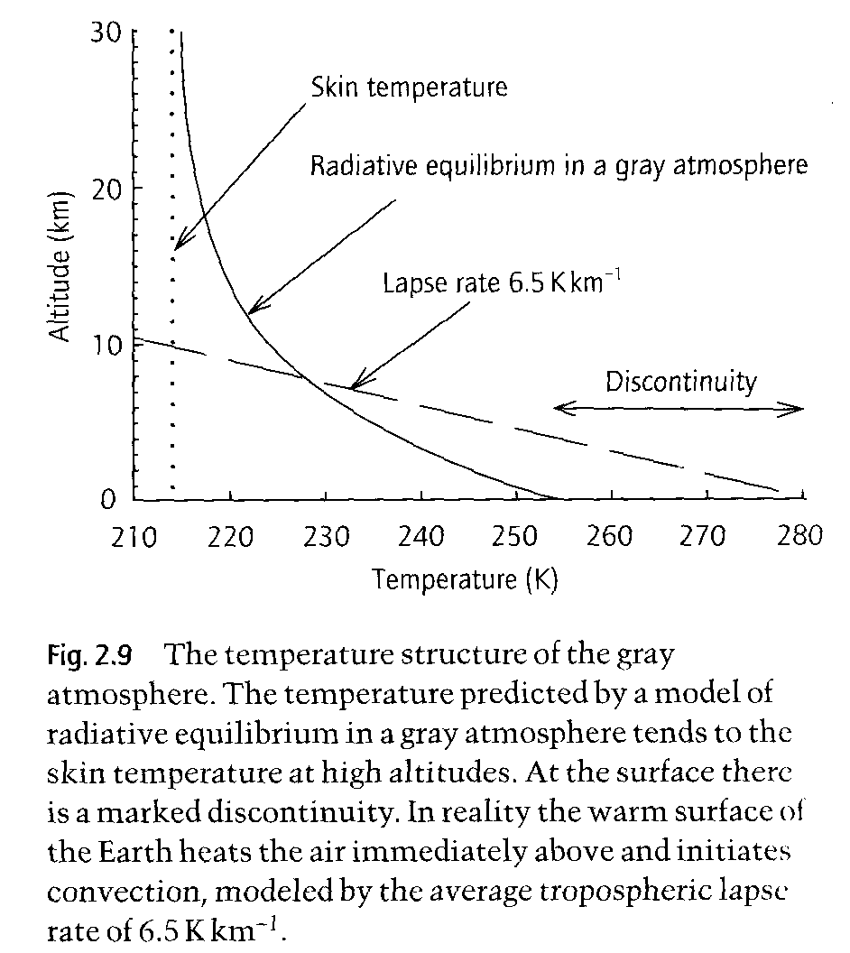
I believe this is wrong. If we go to Venus, the atmosphere the flux from the atmosphere to the surface is not the same has it is from the atmosphere to space. The same is true on Earth (DLR 333 W/m2; TOA OLR 240 W/m2 if you trusted the numbers). However, it is much easier to see that this isn’t true when you think about Venus.
In a non-convective gray atmosphere (ie radiative equilibrium) with no SWR being absorbed by the atmosphere, the difference between the upward flux and downward flux is always equal to the SWR flux being absorbed by the surface. That controls TOA OLR. DLR is depends on the optical thickness of the gray atmosphere at the surface. The mathematics of this is describe here:
http://nit.colorado.edu/atoc5560/week15.pdf
Frank,
Separating the radiative and non radiative energy transfers into two separate ‘loops’ with no net transfer of energy between the two loops solves all those problems.
Frank.
Radiation from an atmosphere taken as a single complete unit must be emitted in all directions equally.
That means radiation down must equal radiation up otherwise the atmosphere can never attain hydrostatic equilibrium. More going down than up means that the upward pressure gradient will always exceed the power of gravity and more going up than down means that the upward pressure gradient will always fall short of the power of gravity.
One of the problems with working with averages, the surface all emits different from equator to pole, from east to west. I’m not sure I completely buy the numbers, but I can see them not being the same, and being different depending where you are.
Quite so, but in the end it must all balance out because indisputably the atmosphere is in hydrostatic equilibrium. It cannot exist otherwise.
Yes, but it’s at least a year, just for the surface asymmetry and tilt.
Frank,
A better way to consider Venus is to account for 100% cloud coverage. Venus is a case of runaway clouds, not runaway GHG’s and the surface in direct equilibrium with the Sun that corresponds to the Earth surface whose temperature we care about is high up in its cloud layer. The hard surface of Venus has more in common with the hard surface of Earth beneath the deep oceans whose temperature has no diurnal or seasonal variability and is dictated by the PVT/density profile of the ocean above. The Venusian CO2 atmosphere weighs nearly as much as Earth’s oceans, the lower portion is in the state of a supercritical fluid and has more in common with an ocean (where heat is stored) than with an Earth like atmosphere.
In a way, Venus is like a mini gas giant. What effect does the Sun have on the solid surface beneath Jupiter’s thick atmosphere?
Stephen wrote: “Separating the radiative and non radiative energy transfers into two separate ‘loops’ with no net transfer of energy between the two loops solves all those problems.”
What evidence – besides words – supports this contention? I’ve already demonstrated that: a) George’s Figure 1 violates Kirckhoff’s Law and b) the S-B equation is only useful when radiation is equilibrium with its surroundings.
The reference I provided provides the solutions for radiative transfer in a gray atmosphere in radiative equilibrium in the absence of convection. If you look at the mathematics, you will find that:
1) OLR at the TOA is always equal to SWR absorbed. (240 W/m2 on Earth)
2) At all altitudes, the difference between upward and downward fluxes is equal to SWR absorbed.
3) Upward and downward fluxes increase linearly with optical thickness (below the TOA) at all altitudes, including the surface.
4) When optical thickness is converted to altitude, curved lines like the one in Figure 2.9
Consequently, DLR is usually NOT EQUAL to TOA OLR in the absence of convection. Unless the mathematics or physics in this reference is wrong. Where do the authors of this standard physics (that can be found in many places) go wrong?
http://nit.colorado.edu/atoc5560/week15.pdf
DLR is not equal to TOA OLR simply because of the action of the non radiative energy loop.
If you treat the non radiative loop as a separate zero sum non radiative energy exchange between surface and atmosphere then radiative balance with space can be indefinitely maintained along with continuing convective overturning.
Stephen wrote: “Radiation from an atmosphere taken as a single complete unit must be emitted in all directions equally. That means radiation down must equal radiation up otherwise the atmosphere can never attain hydrostatic equilibrium. More going down than up means that the upward pressure gradient will always exceed the power of gravity and more going up than down means that the upward pressure gradient will always fall short of the power of gravity.”
If radiation down always equals radiation up, then NO heat can escape from an atmosphere by radiation. That is nonsense. The net flux of radiation is always from hot (the surface) to cold (space). The fluxes can not be equal.
The emission of radiation from a layer of atmosphere thin enough to have a single temperature is the same in both directions. However, absorption is proportional to incoming radiative intensity, which is different because upward radiation is usually coming from where it is warmer.
When you refer to hydrostatic equilibrium, some of the inspiration for your thinking originates with the idea at the temperature gradient in our atmosphere is created by individual molecules losing or gaining kinetic energy (and potential energy) as they move vertically in the atmosphere. However, if you look at the mean free path between collisions and at the average kinetic energy of molecules at atmospheric temperature, you will see that the interconversion of kinetic and potential energy is trivial compared with the kinetic energy being exchanged by collisions in the lower atmosphere. So heat transfer by this type of “molecular diffusion” is incredibly slow, and will be dominated by any FASTER MECHANISM of heat transfer. a) Thermal diffusion – energy transfer by collisions – is faster than molecular diffusion. c) Radiative transfer covers much longer distances at the speed of light. d) Bulk convection is much, much faster than molecular diffusion and it produces exactly the same gradient (-g/Cp) as molecular diffusion.
So there are four potential mechanisms that contribute to the lapse rate in the atmosphere, not just the one you prefer to think about. How do we know which one is responsible for the lapse rate?
The molecular diffusion mechanism should results in enrichment of the of upper troposphere and stratosphere with low molecular weight gases. Enrichment is only observed above the “turbopause” – about 100 km. Figure 2.9 shows what our lapse rate would be if radiative transfer dominated. It doesn’t agree with observation either. So bulk convection is responsible for the Earth’s lapse rate below the tropopause.
Above the turbopause, the lapse rate is not equal to -g/Cp. So molecular diffusion does not control the lapse rate there either, despite enrichment in lighter gases.
The average half-life of a molecule of water vapor in the atmosphere after evaporation is nine days. Molecular diffusion is far too slow to move water vapor (convection of latent heat) to an altitude where clouds form. So the lapse rate we observe in our atmosphere is the result of bulk convection, not molecular diffusion.
Frank,
Are you Doug Cotton ? I have only previously come across such odd ideas about ‘diffusion’. from him.
Radiation upwards from within an atmosphere must escape to space unless absorbed by other radiative material and since our atmosphere is mostly non radiative the majority does escape to space.
You are referring only to the potential energy created by lifting mass against gravity which is indeed relatively trivial. The bulk of the PE arising within a gaseous atmosphere is derived from molecules moving apart against the force of attraction between molecules when they rise upwards along the declining density gradient.
The lapse rate is indeed distorted in every single location away from the ideal as represented by g/Cp but taking the atmosphere as a whole in three dimensions the g/Cp formula must be satisfied otherwise no hydrostatic equiolibrium.
Frank,
In relation to Venus you make the same mistake as Trenberth did in relation to Earth.
You include energy arriving back at the surface from non radiative processes within the downward radiative flux.
George’s piece is telling you why you cannot do that.
George said this in the head post:
“Trenberth’s energy balance lumps the return of non radiant energy as part of the ‘back radiation’ term, which is technically incorrect since energy transported by matter is not radiation”
Exactly.
Frank,
What is your conceptualization of physics of the GHE?
Mine is this definition here from Wikipedia:
The greenhouse effect is a process by which thermal radiation from a planetary surface is absorbed by atmospheric greenhouse gases, and is re-radiated in all directions. Since part of this re-radiation is back towards the surface and the lower atmosphere, it results in an elevation of the average surface temperature above what it would be in the absence of the gases.[1][2]”
Emphasis on the word part in the second sentence. Note, there is no mention of DLR at the surface, and note also the verbiage ‘back towards the surface’ (and not necessarily back to the surface).
I agree actual DLR at the surface is roughly 300 W/m^2, but the atmosphere itself has essentially 3 separate energy sources or 3 separate energy flux inputs. Only one of them is the fraction of the surface emitted IR flux density which is absorbed by the atmosphere, i.e. what George is quantifying as ‘A’. The other two energy sources are post albedo solar power absorbed by the atmosphere and the latent heat of evaporated water moved non-radiantly from the surface into the atmosphere (which drives weather and condenses to form clouds). The total DLR at the surface will have contributions or be sourced from all 3 energy inputs to the atmosphere — not just the IR flux emitted by the surface which is absorbed. The point being all of the energy fluxes into the atmosphere contribute to both upward IR push and the downward IR push occurring.
My conceptualization of the GHE doesn’t much involve or isn’t centered on the total DLR at the surface. I simply see the surface as the lowest point the energy of a downward re-emitted photon (from the initially absorbed surface IR flux) could potentially pass back to before it’s reabsorbed and (likely) re-radiated again. Most of the time, such a downward re-emitted photon is reabsorbed at a lower point well above the surface (and doesn’t travel very far before being reabsorbed). Furthermore, my conceptualization is equally focused (if not more so) on the massive upwelling IR (and upward non-radiant/convective) push the system makes in order to achieve radiative balance with the Sun at the TOA. After all, to satisfy the 2nd Law, the net flow of energy must be up and out the TOA (which it is). What I conceptualize is this massive upward push being slowed down or ‘resisted’ by the fact that absorbed upwelling IR from the surface is re-radiated both up and down — the downward portion being re-absorbed at a lower point, causing/forcing the lower atmosphere and ultimately the surface to emitting at higher rates (higher than 240 W/m^2) in order for the surface and the whole of the atmosphere to pushing through the required 240 W/m^2 of IR back into outer space. To me, the total DLR at the surface is mostly just what happens manifest when all of the effects are mixed together (radiant and non-radiant) in order for the surface and the whole of the atmosphere — driven by this above underlying mechanism — to be pushing through the required 240 W/m^2 back out to space.
Remember also, not all of the DLR at the surface is actually added to the surface, since some of it is short circuited (or cancelled) by non-radiant flux leaving the surface, but not flowing into the surface (as non-radiant flux). This makes its effect and/or possible influence or contribution to the GHE and its raising of the surface temperature even more fuzzy and imprecise.
I assume you agree that the constituents of the of the atmosphere, i.e. GHGs and clouds, act to both cool the system and ultimately the surface by emitting IR up towards space and act to ultimately warm the system and surface by emitted IR downward towards the surface. Right?
George is saying like anything else in physics or engineering, this has to be accounted for, plain and simple. The re-radiation of the surface IR energy captured by ‘A’ is henceforth non-directional (is re-radiated both up and down), no matter where the energy goes or how long it persists in the atmosphere. The problem is the thermodynamic path manifesting the energy balance is far too complex and non-linear to trace the path of the energy and quantify how much of A is actually ultimately driving enhanced surface warming. Hence what the black box model exercise here is doing:
http://www.palisad.com/co2/div2/div2.html
It’s just a means of quantifying for this effect even though there is no way to trace the path of A within the complex thermodynamic path, so far as its ultimate contribution in driving enhanced surface warming. It is NOT an emulation of the thermodynamics manifesting the balance, and would surely be spectacularly wrong if it were. It tells us essentially nothing about why the surface energy balance is what it is.
Frank,
Central to the point or dispute here is the field considers both +3.7 W/m^2 of post albedo solar power entering the system and +3.7 W/m^2 of GHG absorption to have the same *intrinsic* surface warming ability. That is, each is said to have a ‘no-feedback’ surface temperature of about 1.1C, which is derived from this formula for added GHGs:
dTs = (Ts/4)*(dE/E), where Ts is equal to the surface temperature and dE is the change in emissivity (or change in OLR) and E is the emissivity of the planet (or total OLR).
Plugging in 3.7 W/m^2 for 2xCO2 for the change in OLR, we get dTs = (287K/4) * (3.7/239) = 1.11K
The problem is there is nothing implicit in this formulation that the variable ‘OLR change’ be an instantaneous change. All this formula really does is multiply the 3.7 W/m^2 by the 1.6 to 1 power densities ratio between the surface and TOA (385/239 = 1.61) and add the result back to the baseline of 385 W/m^2 and convert back to temperature (or divide by the emissivity, add and convert). Really all it does is validate the T^4 relationship between temperature and power between the surface and TOA boundaries, and that’s it. The 1.6 to 1 power densities ratio between the surface and the TOA is specifically that offsetting post albedo solar power entering the system and is not connected, physically or mathematically, to an amount offsetting GHG absorption. That is, the ratio’s physical meaning is that it takes about 1.6 W/m^2 of net surface gain to allow 1 W/m^2 to leave the system at the TOA, offsetting each 1 W/m^2 entering the system (post albedo) from the Sun.
The concept of ‘zero-feedback’ is (or at least should be) a linear increase in aggregate dynamics. Specifically, a linear increase in aggregate dynamics required to establish equilibrium with space. For +3.7 W/m^2 of post albedo solar power entering the system, the 1.1C is a correct measure of a linear increase in aggregate dynamics in response, but it’s not for +3.7 W/m^2 of GHG absorption. Though of course since both will result in a -3.7 W/m^2 TOA deficit, you can apply the calculation of the former to the latter and it will indeed restore balance as claimed, but that’s trivially true. Moreover, it’s not related in anyway to how the GHE, mechanistically, actually works or is physically driven.
The key point is whether the field realizes it or not, if both +3.7 W/m^2 of GHG absorption and +3.7 W/m^2 of post albedo solar flux are established to have the same ‘no-feedback’ surface temperature increase (which they are), then it’s effectively being claimed the *intrinsic* surface warming ability of each is equal to one another.
In which case, in order to be true or valid, the rules of linearity must be applied equally to each, otherwise one is not a measure of the same thing as it is for the other. Though again, in both cases there is a -3.7 W/m^2 TOA deficit that has to be restored, so you can apply the calculation of a linear increase in adaption for +3.7 W/m^2 of post albedo solar power entering of 1.1C to +3.7 W/m^2 of GHG absorption and it will restore balance as claimed.
Ultimately, you really need to tie the quantification of the *intrinsic* surface warming ability of +3.7 W/m^2 of GHG absorption to dynamics — specifically aggregate dynamics, otherwise it doesn’t have a true mechanistic connection to greenhouse warming of the surface, or more specifically a linear increase in greenhouse warming of the surface in response, which is clearly what it logically should be.
Aggregate GHG absorption in the steady-state prior to changing anything is around 300 W/m^2 (George’s A value in W/m^2), for which it only takes about +150 W/m^2 net surface gain to offset this captured flux (390-240 = 150). By ‘offset’, I simply mean to establish equilibrium with space. If the system adapts linearly, where the same rules of linearity are followed as they are for post albedo solar power entering the system, it only takes about 0.55C of surface warming to restore balance at the TOA, and that this is really a proper starting point to work from regarding the sensitivity (and not the 1.1C ubiquitously cited by the field).
Frank,
In a nutshell — if George has a valid case for a factor of 2 starting point error, the field (i.e. those in the field and people like yourself) seems unable to conceptually separate the underlying driving physics of the GHE from the actual thermodynamic path — in particular the radiative transfer component — manifesting the energy balance, and how it (the underlying driving physics) affects the adaption of the system to an imbalance imposed by added GHGs; and what is or *should be* the proper quantification of a linear increase in that adaption compared to a linear increase in adaption for post albedo solar power entering the system (for the quantification of *intrinsic* surface warming ability). The error, if he’s right, is really just one of a failure to apply the rules of linearity equally for each.
The upper limit is it adds linearly. It’s just not linear, it’s nonlinear and adds very little due to water vapor overwhelming co2.
George,
“The purpose was to separate the radiation out, model how it should behave by extracting the transfer function between surface temperature and planet emissions, test the resulting model with data measuring what is being predicted and if the model correctly describes the relationship between the surface temperature to the planets emissions into space, it also must quantify the sensitivity, which the IPCC defines as the incremental relationship between these two factors. This whole exercise is nothing more than an application of the scientific method to ascertain a quantitative measure of the sensitivity which to date has never been done.”
While I think I understand this quite well, I think the vast majority don’t know where you’re coming from with all of this. There needs to be a foundation laid out of the methods behind the derivation of your equivalent model here, which is the starting point of the analysis. Most everyone seems totally faked out by it. They think it’s claiming to emulate and be a model of the immense dynamical complexity of the actual thermodynamics and thermodynamic path manifesting the energy balance, involving the transient mixing of radiant and non-radiant energy in a highly non-linear way, where one thing incrementally affects the other up and down through the whole atmosphere. This is not what it is and not what’s it’s doing, but they don’t understand and see this. They don’t understand what the model is actually doing and quantifying. Without fully understanding it, they don’t understand how it relates to the data plot and what it reveals about the sensitivity.
I posted a link to this article at SoD when it was first put up, and some people there may even be following this thread, but laughing their heads off at what they are perceiving as spectacular nonsense. Again, they think your model is some sort of emulation of the actual thermodynamic path manifesting the energy balance, or trying to say why the balance is what it is (or has physically manifested to what it is). The model of course is not doing this, but they fundamentally DO NOT UNDERSTAND THIS.
Like I say, more groundwork needs to be laid out on the foundation of the derivation of your model before anyone is likely to even begin to understand this and ultimately how it relates to the sensitivity.
Funny this has been at the foundation of electronic design simulation. From the early 90’s. Only 25 years ago.
Well that may be true, but it seems very few understand the foundation behind how he’s deriving his model.
Steve Wilde and George White: George White goes wrong in his opening paragraph:
“Wikipedia defines a Stefan-Boltzmann gray body as one “that does not absorb all incident radiation” although it doesn’t specify what happens to the unabsorbed energy which must either be reflected, passed through or do work other than heating the matter. This is a myopic view since the Stefan-Boltzmann Law is equally valid for quantifying a generalized gray body radiator whose source temperature is T and whose emissions are attenuated by an equivalent emissivity.”
Wikipedia’s view is not myopic for the following reason: Imagine a gray body with emissivity less than 1 completely surrounded by a blackbody with emissivity equal to 1. To avoid problems with viewing angles, let’s imagine a negligible gap under vacuum between a spherical gray body and a spherical blackbody cavity. The gray body emits less energy than the black body and therefore will become warmer if it absorbs all of the radiation emitted by the blackbody. Heat will flow from cooler to warmer. Put the blackbody on the inside and the graybody surrounding it and heat will flow the other direction. Common sense (and Kirckhoff’s Law) says the the gray body must reflect/scatter enough of the incoming radiation so that emissivity = absorptivity.
So even Figure 1 has serious problems. If the graybody filter has an emissivity less than 1, then Kirckhoff’s Law demands that some of the radiation from the blackbody earth be reflected/scattered back to the surface.
Of course, this seems like nonsense because the atmosphere doesn’t have any surface from which incoming radiation can be scattered. However, it doesn’t have a surface to scatter radiation on the way to space either, and therefore can’t have an emissivity less than 1.
These problems develop because you are trying to apply the S-B eqn to a situation where it doesn’t apply. The derivation of Planck’s Law assumes that radiation is in equilibrium with the matter (originally quantizer oscillators) which it is passing through. That produces a nice smooth curve when radiation intensity is plotted vs wavelength for a given temperature. We know that thermal IR does not reach equilibrium with the atmosphere on its way to space; Some wavelengths pass straight through. The intensity vs wavelength plot is not smooth.
When you integrate Planck’s Law over all wavelengths, you get the S-B equation with e = 1. What makes emissivity less than 1? Scattering at surfaces, which is why emissivity = absorptivity. Scattering is the same in both directions. Some people think the reason emissivity can be less than 1 is because a graybody doesn’t emit at some wavelengths. However, if an object doesn’t emit at some wavelength, then it doesn’t absorb at that wavelength either and it is semi-transparent.
With semi-transparent objects, you aren’t dealing with radiation in equilibrium with the material it is passing through. Planck’s Law and the S-B eqn don’t apply. You need to use the Schwarzschild equation.
Frank,
Separating the radiative and non radiative energy transfers into two separate ‘loops’ with no net transfer of energy between the two loops solves all those problems.
Frank,
George is just saying the atmosphere more or less just acting a filter between the surface and space, where of the 385 W/m^2 emitted from the surface, only 240 W/m^2 is emitted to space. The data he’s plotted is measured and thus automatically accounts for all the effects, radiant and non-radiant, known and unknown, that occur in the atmosphere to ultimately manifest this end result.
Again, it’s not the physical law itself, in and of itself, that constrains the sensitivity to within the bounds of the grey body curve.
Why this is so elusive to you is because it seems you have accepted the fundamental way the field has framed up the feedback and sensitivity question, which is really as if the Earth-atmosphere system is a static equilibrium system (or more specifically a system that has dynamically a reached a static equilibrium), and whose physical components’ behavior in response to a perturbation or energy imbalance will subsequently dynamically respond in a totally unknown way with totally unknown bounds, to reach a new static equilibrium. This is effectively the way the field has framed up the issue.
The system is an immensely dynamic equilibrium system, where its energy balance is continuously dynamically maintained. It has not reached what would be a static equilibrium, but instead reached an immensely dynamically maintained approximate average equilibrium state. It is these immensely dynamic physical processes at work, radiant and non-radiant, know and unknown, in maintaining the physical manifestation of this energy balance, that cannot be arbitrarily separated from those that will act in response to an imposed imbalance on the system, like from added GHGs.
It is physically illogical to think these physical processes and feedbacks already in continuous dynamic operation in maintaining the current energy balance, like those of water vapor and clouds, would have any way of distinguishing such an imbalance from any other imbalance imposed as a result of the regularly occurring dynamic chaos in the system, which at any one point in time or in any one local area is almost always out to balance to some degree in one way or another.
It is this logic in conjunction with the decades long dynamic measured response curve George has plotted, composed of dots of monthly averages per grid area, that so closely conforms to what he’s saying/claiming regarding the law; and that there’s no reason to think the incremental response of the system to a newly imposed imbalance, let alone a very small one like from added GHGs, would be radically different from or diverge out of the bounds of this curve.
RW,
That seems to me to be a pretty good summary of what George is doing.
I’ve tried to push a step further but thus far George prefers to leave the matter of the actual stabilising mechanism behind it all as undetermined.
The key point seems to be that AGW theory conflates DWIR which is atmospheric energy returning to the surface by radiative means AND atmospheric energy returning to the surface by non radiative means. The latter involves retrieval of KE from PE as one descends along the lapse rate slope.
The AGW theory, being purely radiative, cannot conceive of surface IR being prevented from radiating to space as a result of conduction at and convection from the surface. They seem to insist that surface IR can be in two places at once i.e. being radiated and conducted/convected simultaneously but that is a clear breach of conservation of energy.
The conceptual solution is to propose separate energy loops for the radiative and non radiative components of the basic energy fluxes. George accepts the principle of a closed zero sum up and down energy loop which I say is what drives continuing convective overturning. The presence of that closed loop is what causes the mass induced greenhouse effect in my view.
The problem everyone seems to have is envisaging how the non radiative component can raise surface temperature above S-B as a result of atmospheric mass convecting within a gravity field.
The best way to look at it is by recognising that conduction and convection are slower forms of energy transfer than radiation so the time taken by solar energy to pass through those processes MUST raise surface temperature above S-B.
Still, I think George’s contribution is very helpful, expecially in supporting my earlier work which pointed out Trenberth’s error in thinking that he could just increase DWIR to balance non radiative latent heat and thermals.
What really happens is that KE appears as if by magic from PE as one descends along the lapse rate slope in descending columns of air and disappears as if by magic from KE to PE in ascending columns. Rather than being magical it is just a reflection of the different forms of energy represented by KE and PE. It is non contentious that moving mass vertically within a gravity field transforms rather than moves energy. That is a basic principle of meteorology.
The energy remains present within the atmosphere but PE cannot be sensed as heat.
Therefore the surface temperature is comprised of two elements namely:
i) 255K from solar energy passing through the Earth system.
ii) 33K via KE (heat) appearing from PE (not heat) within descending convective columns and then being circulated around the surface so that it is effectively an addition to the radiative component which arises from solar energy.
Putting ii) into the DWIR figure is a gross error which completely obscures the reality because it assumes that non radiative energy returns to the surface by radiative means which is clearly a nonsense.
Infra red sensors receive both radiation from the sky above AND radiation from the KE at the point along the lapse rate slope at which the measurement is taken.Only the former should be taken as radiation from the sky. The latter is the level of radiation that has been recovered from non radiative processes at that specific point along the lapse rate slope and at the surface that temperature enhamcement from recovered KE is 33K
That is why George’s approach comes up with the much lower figure for DWIR than does Trenberth. George is correctly calculating just the sky radiation without that additional component of KE recovered from PE along the lapse rate slope.
AGW theory overestimates GHG sensitivity because it adds the sky radiation to the KE recovered along the lapse rate slope and attributes the KE recovered along the lapse rate slope to GHGs which is incorrect. The radiation from GHGs is only involved in the sky radiation alone.
“..those processes MUST raise surface temperature above S-B.”
Never above S-B, always equal S-B whether global 255K up to current around 289K or any other steady state energy budget balance imagined.
“Never above S-B, always equal S-B”
Yes, but SB doesn’t drive or set the temperature, it’s just the required physical law (including an effective emissivity) that all radiating bodies who radiate energy consequential to its temperature must obey. This was my hypothesis and figure 3 was a test of it.
Correct.
But note that a surface beneath a convecting atmosphere need not radiate to space according to its temperature due to the energy drawn into, and subsequently permanently locked into, recurring non radiative processes by conduction and convection in the vertical column.
The same parcel of energy cannot be radiated to space at the same time as it is being conducted and convected within the vertical column otherwise one breaches conservation of energy.
AGW theory requires surface energy to travel to two separate destinations simultaneously. That is the unavoidable consequence of ignoring the energy requirement of non radiative processes.
George’s work has highlighted that issue very nicely.
“But note that a surface beneath a convecting atmosphere need not radiate to space according to its temperature..”
A good example of Stephen’s imagination unconstrained by known S-B testing and theory. The near surface atm. always radiates toward space according to its temperature Stephen. And at all wavelengths. All the time.
Frank,
The radiative GHE, atmospheric radiative transfer, the Schwartzchild eqn., increases in GHGs leading to enhanced surface warming — it’s all valid theory according to George. He’s only ultimately claiming the sensitivity or the predicted ranges of sensitivity supported by the IPCC are way too high and his methods (designed to eliminate heuristics as much as possible) derive far lower sensitivity. That’s really all. There’s no radical new, transformative knowledge being put forth here.
He’s just applying basic, well established techniques (and logic) one would use to reverse engineer an unknown, but measurable system. I don’t why so many people such as yourself find it so hard to grasp what he’s doing, but perhaps more foundational groundwork needs to be laid out for the methods being employed.
“He’s only ultimately claiming the sensitivity or the predicted ranges of sensitivity supported by the IPCC are way too high and his methods (designed to eliminate heuristics as much as possible) derive far lower sensitivity.”
Exactly, nothing more and nothing less, although the analysis does lead to a lot more. The question for Frank is how does the data support a sensitivity different from that of the gray body model I use to predict the measured LTE relationship between the surface and TOA?
Asserting that the data doesn’t represent the sensitivity would mean that the IPCC definition is wrong which is defined as the incremental relationship between the surface temperature (equivalent to its emissions) and the radiant behavior at TOA and these are the only 2 observables being modeled.
The point is that as long as I can predict the bulk behavior of the system with a reasonably accurate model, how the atmosphere manifests this behavior is irrelevant to the model.
The flaw of climate science is assuming the atmosphere drives the surface temperature, when in fact, the Sun drives the surface temperature and the atmosphere comes along for the ride contributing a little extra warmth be delaying some surface emissions and returning them the surface via GHG’s and clouds (the ‘and clouds’ is crucial to understanding). The delay is important and to how old energy and new energy can be added to give the appearance of more energy than the Sun is providing.
“The flaw of climate science is assuming the atmosphere drives the surface temperature..”
This is no flaw, it is just physics as shown by your Fig. 2 with different Earth atm. emissivity A gray body with sun load and albedo held constant.
“This is no flaw, it is just physics as shown by your Fig. 2 with different Earth atm. emissivity A gray body with sun load and albedo held constant.”
More precisely, the Sun is the only thing that drives the surface temperature. The grayness of the atmosphere recycles some of the surface emissions back making the surface warmer than it would be based on solar input alone. The real flaw is considering a 1 W/m^2 increase in absorption drives the system in the same manner as 1 W/m^2 more from the Sun.
“the Sun is the only thing that drives the surface temperature….The grayness of the atmosphere recycles some of the surface emissions back making the surface warmer than it would be based on solar input alone.”
Thus the sun, albedo AND grayness of the atm. all drive (make, balance, etc) the surface temperature of a planet (or moon, dwarf planet etc.) as your Fig. 2 shows. The grayness is usually discussed as the atm. optical depth. Convection and evaporation cancel out, have no or negligible effect on global surface temperature over long periods (4 to 10 years or more). Your sensitivity to CO2 is manifested as changes in optical depth (grayness).
PS: Recycling is not exact wording, a photon absorbed is annihilated, an emitted photon is born anew not recycled.
“PS: Recycling is not exact wording, a photon absorbed is annihilated, an emitted photon is born anew not recycled.”
OK, so to be more specific, lets say recycling energy since recycling is ‘green’.
Frank,
“Wikipedia’s view is not myopic for the following reason:”
Your counter example is a bit contrived. Can you offer a physical realization of this, complete with all fluxes? If you do, you will find that there is no contradictions. In fact, a gray body on the inside of a BB radiator will converge to the temperature of the BB at equilibrium, independent of it’s grayness.
Also, as I pointed out, figure 1 is to conform to the wiki view, while figure 2 shows the actual fluxes flowing through the system.
You may try to assert that SB doesn’t apply, but the data defies this assertion. Part II of the question at the end was to explain the measured relationship in another way that can support an insanely high sensitivity.
Frank,
“The same is true on Earth (DLR 333 W/m2; TOA OLR 240 W/m2 if you trusted the numbers).”
Not that it’s all that critically important, but Trenberth’s numbers are almost certain to be wrong for DLR at the surface. Do you really think that the only way a joule can pass from the atmosphere to the surface is via EM radiation? The non-radiant fluxes he depicts, i.e. 80 W/m^2 of latent heat, and 17 W/m^2 of ‘thermals’, are NOT the net fluxes (i.e. not up minus down at the surface), but are instead the gross fluxes leaving the surface. Read the paper again if you think otherwise.
DLR at the surface is probably more like 300 W/m^2 (or maybe somewhere in the high 200s). Depicting that the only way a joule can pass to the surface is by radiation is wrong because the latent heat from evaporation is largely (or at least somewhat) offset at the surface by the heat of condensed water in precipitation and clearly not offset at the surface solely by radiation, i.e. not offset solely by DLR at the surface.
”The non-radiant fluxes he depicts, i.e. 80 W/m^2 of latent heat, and 17 W/m^2 of ‘thermals’, are NOT the net fluxes (i.e. not up minus down at the surface), but are instead the gross fluxes leaving the surface.”
Agreed. The total W/m^2 (80+17 here) is the energy transfer per second per unit area – a total of (radiative+conductive+convective transfers) there is no need to separate the individual mode of transfer. Likewise there are 80+17 returning to surface as none of this (rain or wind) energy is stored long term in the ~saturated atm., the net up minus down is net flux of zero over 4-10 years these energy budgets are constructed. This flux is therefore correctly & simply included in the 333 all sky emission to surface.
“This flux is therefore correctly & simply included in the 333 all sky emission to surface.”
Ok, this is a critical point i.e. whether it is ‘correct’ to include the downward radiative flux from the retrieval of KE from PE via non radiative processes along the lapse rate slope together with the radiative flux from GHGs in the atmosphere in the total figure for DWIR reaching the surface as Trenberth and the entire AGW establishment have done.
The whole issue of the scale of anthropogenic climate change hinges on that single point.
Well, it depends what you are using the data for.
If one is trying to establish the climate sensitivity to GHGs (ignoring for the moment any stabilising processes that may or may not be acting in the background) then it is plainly wrong to add the DWIR derived from KE returning from non radiative processes to the DWIR emanating directly from GHGs.
It is even worse if you add it to the DWIR from CO2 alone since CO2 is only a small fraction of the entire radiative capability of our atmosphere.
By adding the DWIR from the non radiative processes to the DWIR from CO2 and then treating the combined total as coming from CO2 gives an outrageously inflated number for climate sensitivity to CO2.
”and then treating the combined total as coming from CO2..”
No one does that Stephen, your outrageous claim is unfounded. No competent study has ever claimed the TFK09 333 is from CO2 alone in sensitivity studies or any kind of study.
The combined total 333 DWIR in TFK09 is global energy balance per sec. per unit area from a hemisphere of directions crossing the lower boundary of the atm. column from all sky emission. All sky! The energy flux is steady state over long periods (4-10 years or more). Updrafts and LH put the “cycle” in hydrological with downdrafts and rain.
So what do you say is the proper split between DWIR emanating from the radiative absorption properties of CO2, the DWIR emanating from the radiative absorption properties of all other radiative material in the atmosphere and separately, the DWIR emanating from KE retrieved from PE via non radiative processes which has been then passed to CO2, and other radiative material in the atmosphere via conduction along the line of the lapse rate slope.
I don’t think anyone has ever looked at that .
Co2 adds 2.7 (3.7?)w/m^2, I suspect it could very higher during the day when everything is hot and radiating, but that probably the average, they average all the useful data away.
As for your other, I do calculate the enthalpy of the dry air, and the then the enthalpy from the water content separately. Plus calculate solar at every surface station in the data set. http://sourceforge.net/projects/gsod-rpts/
Is all in the beta report folder.
Micro6500
How do you distinguish between the portion of the CO2 molecule temperature that is attributable to absorption of IR from the surface as compared to the portion arising simply from its position along the lapse rate slope (the non radiative portion)?
That is important because if a CO2 molecule sits at its correct temperature along the lapse rate slope then there is a zero component attributable to absorption of surface IR
If it then absorbs IR from the surface it will no longer be in its correct position (too warm) and will be forced to rise but if it does rise it will cool back to the correct temperature for its position via conduction to colder adjoining molecules so again the contribution to its temperature from surface IR will be zero.
If it radiates to space (in ANY wavelength – it doesn’t need to radiate in the ‘blocked’ wavelength) then it will cool and no longer be in its correct position along the lapse rate slope and will fall until it is back in the correct position with, again a zero contribution from surface IR.
Do you see the problem?
AGW theory appears to say that ALL the thermal energy (KE) in the CO2 molecule is from surface emssions that are prevented from leaving to space. The fact that it would be at much the same temperature anyway as a result of its interaction with non radiative processes appears to have been ignored.
Okay, yeah that wasn’t what I was thinking about. But I think your conclusion sums it up, it won’t look abnormal, the whole column will be working to equilibrium, just slightly warmer.
And it’s a good point that the open window is still radiating and conduction will move blocked energy down into that window over time.
Trick,
“This flux is therefore correctly & simply included in the 333 all sky emission to surface.”
Yes, this is what Trenberth does, but the point is that the non radiative fluxes have nothing to do with how much energy the planet will emit, nor do they have an effect on the sensitivity. Any effect they have on the temperature is already included in the final surface temperature and the consequential radiant emissions. So, relative to trying to understand how radiative fluxes tell us what the sensitivity is, including non radiant flux in the balance is superfluous, misleading and obfuscatory.
Yes, I mostly agree 8:11am – that is what your Fig. 2 is telling you. As I calculated:
https://wattsupwiththat.com/2017/01/05/physical-constraints-on-the-climate-sensitivity/#comment-2390884
all that matters to increase global surface temperature above 257K N2/O2 alone to 290.7K ~today is the increase of the atm. emissivity (your A) from N2/O2 (I used 0.05) up to A of 0.80 existing on avg. in the global atm. currently.
You could add in TFK09 (80+17) UP then subtract (80+17) DOWN in balance steady state superposed independent energy flux on Fig. 2 as Trenberth does for no change in the 290.7K I calculated & that is not in any way superfluous, misleading or obfuscatory, it is what observations of nature are telling you.
Stephen Wilde January 14, 2017 at 9:19 am
Micro6500
How do you distinguish between the portion of the CO2 molecule temperature that is attributable to absorption of IR from the surface as compared to the portion arising simply from its position along the lapse rate slope (the non radiative portion)?
That is important because if a CO2 molecule sits at its correct temperature along the lapse rate slope then there is a zero component attributable to absorption of surface IR
If it then absorbs IR from the surface it will no longer be in its correct position (too warm) and will be forced to rise but if it does rise it will cool back to the correct temperature for its position via conduction to colder adjoining molecules so again the contribution to its temperature from surface IR will be zero.
If it radiates to space (in ANY wavelength – it doesn’t need to radiate in the ‘blocked’ wavelength) then it will cool and no longer be in its correct position along the lapse rate slope and will fall until it is back in the correct position with, again a zero contribution from surface IR.
Do you see the problem?
Yes, you don’t understand the kinetic theory of gases or the internal energy structure of molecules.
The energy is in three forms: translational (unquantized), rotational and vibrational (both quantized).
Temperature is due to the KE in the translational mode, at temperatures around 300K most of the molecules will be in the ground vibrational state but will be distributed among various rotational states. When a CO2 molecule absorbs an IR photon it is excited to a higher vibrational and rotational level but its translational energy is unaffected! The molecule loses that excess energy either by emitting a photon or collisional deactivation by neighboring molecules, emitting a photon will not change the translational energy of the molecule.
Phil,
You seem to be suggesting that a CO2 molecule does not change temperature when receiving IR from the ground or releasing IR to the ground because the translational energy is unaffected and translational energy alone determines temperature.
Is that what you are saying ?
Stephen Wilde January 15, 2017 at 12:50 am
Phil,
You seem to be suggesting that a CO2 molecule does not change temperature when receiving IR from the ground or releasing IR to the ground because the translational energy is unaffected and translational energy alone determines temperature.
Is that what you are saying ?
It’s not a suggestion it’s a fact!
I don’t think you have that right:
“The kinetic energy of gas molecules depends only on their temperature. Pressure depends on both temperature and number density. If you have two samples of gas at the same temperature but one is 1/1000th of an atmosphere and one is 10 atmospheres in pressure the molecules will have the same average energy. The translational, rotational, and vibrational motion COMBINE as the total kinetic energy of the molecules.”
from here:
http://en.allexperts.com/q/Physics-1358/2008/11/energy-levels.htm
Stephen Wilde January 15, 2017 at 6:00 am
I don’t think you have that right:
Yes I do, I suggest you refer to a undergrad text on Physical Chemistry,
“The thermodynamic temperature of any bulk quantity of a substance (a statistically significant quantity of particles) is directly proportional to the average—or “mean”—kinetic energy of a specific kind of particle motion known as translational motion. These simple movements in the three x, y, and z–axis dimensions of space means the particles move in the three spatial degrees of freedom. This particular form of kinetic energy is sometimes referred to as kinetic temperature. Translational motion is but one form of heat energy and is what gives gases not only their temperature, but also their pressure and the vast majority of their volume. This relationship between the temperature, pressure, and volume of gases is established by the ideal gas law’s formula pV = nRT and is embodied in the gas laws.
The extent to which the kinetic energy of translational motion of an individual atom or molecule (particle) in a gas contributes to the pressure and volume of that gas is a proportional function of thermodynamic temperature as established by the Boltzmann constant (symbol: kB). The Boltzmann constant also relates the thermodynamic temperature of a gas to the mean kinetic energy of an individual particle’s translational motion as follows:
Emean = 3⁄2kBT
where…
Emean is the mean kinetic energy in joules
kB = 1.3806504(24)×10−23 J/K
T is the thermodynamic temperature in kelvins”
Nothing there that suggests that translational energy is not affected by an increase in the other two forms of energy.
wildeco2014 January 15, 2017 at 8:53 pm
Nothing there that suggests that translational energy is not affected by an increase in the other two forms of energy.
Again it’s time for you to study some physical chemistry!
For a CO2 molecule to absorb a photon the energy of the photon has to be exactly equal to the energy difference between the energy level it occupies (rot/vib) and the energy level it is promoted to (rot/vib), there’s none left over to increase the translational energy.
The link I gave you refers to the combination of all three types contributing to kinetic heat and thus temperature
wildeco2014 January 16, 2017 at 7:59 am
The link I gave you refers to the combination of all three types contributing to kinetic heat and thus temperature
Yes and it’s wrong. Since you appear to have an aversion to text books try here:
http://hyperphysics.phy-astr.gsu.edu/hbase/Kinetic/kintem.html
“The kinetic temperature is the variable needed for subjects like heat transfer, because it is the translational kinetic energy which leads to energy transfer from a hot area (larger kinetic temperature, higher molecular speeds) to a cold area (lower molecular speeds) in direct collisional transfer.”
http://hyperphysics.phy-astr.gsu.edu/hbase/thermo/temper.html
“Temperature is not directly proportional to internal energy since temperature measures only the kinetic energy part of the internal energy, so two objects with the same temperature do not in general have the same internal energy”
http://teacher.pas.rochester.edu/phy121/lecturenotes/Chapter18/Chapter18.html
“18.4. Translational Kinetic Energy
The calculation shows that for a given temperature, all gas molecules – no matter what their mass – have the same average translational kinetic energy, namely (3/2)kT. When we measure the temperature of a gas, we are measuring the average translational kinetic energy of its molecules.”
It does seem counterintuitive that any number of IR photons from the ground can hit a CO2 molecule and thus increase vibrational and rotational energy without also affecting translational energy / temperature as a result.
I don’t think you have yet provided a source for the proposition that increasing vibrational and rotational energy does not as a side effect also increase translational energy.
It appears that rotational and vibrational energy can affect the temperature of the system in which they are found via an effect on the entropy of the system.
Assessing the temperature of an individual molecule is also problematic because such temperature depends on its relationship with other surrounding molecules via pressure and internal energy differentials.
https://www.quora.com/Does-the-vibrational-rotational-energy-of-a-molecule-contribute-to-the-temperature-of-the-molecule
“Temperature is, roughly, a statistical entity which applies to systems with many bodies. In that sense it is difficult to speak about the temperature of a molecule (difficult but not completely wrong).
It is defined as the mean energy of all constituents (molecules in the case of your question). So yes, the rotational energy of molecules does impact the temperate of the system they are in.”
Furthermore, it appears that when collisions occur all three types of kinetic energy can interchange with each other to affect temperature:
https://www.quora.com/Can-vibrational-rotational-energy-of-a-molecule-be-interconvertible-with-a-molecules-translational-energy
“Yes, as in my answer to a similar question, when molecules collide with each other or with the walls of a container all sorts of energy interchanges can take place as the particle bounces off whatever it ha collided with.
A single particle in deep space will maintain its distribution of various energies for a long time but eventually it will collide with something and lose kinetic energy (presumably he means translational energy) and gain vibrational and/or rotational energy.”
So, I don’t accept that the truth is as simple as there being no effect on the temperature of a CO2 molecule when it absorbs and re emits longwave IR from the ground, which is what you are trying to assert.
Not quite, it has the normal affect, but since the control of the engagement of the lower net outgoing radiation mode it dependant on higher levels of rel humidity, and that is a temperature effect. So if it was an extra 4F max temperature because it was sunny, most land locations don’t have a lot of excess water to evaporate, so you don’t get a lot of added water to your dew point. Once the sun goes down since dew point temperature didn’t go up, it cools that 4F at the high cooling rate, only after most of it is gone the transition to the low cooling rate will happen. If it’s 8F, stays in high cooling even longer.
I think based on enthalpy changes, as absolute humidity goes up, both cooling rates drop some, this is highlighted by deserts that have about 50%more kJ avg lost at night than tropics, yet have almost twice the stored energy, it’s just the effect of the percentage of high cooling rate to low cooling rates.
The affect of co2’s ghg effect is just muted by outgoing radiation water vapor temperature regulation.
This is why I think adding more ghg will have a smaller affect on min temp than I think George estimates. What my hypothesis would be subject to is the ghg effect added to the slow rate, but only on the residual energy after full slow rate engages.
In the fall, any accumulated energy would bleed off as there was a longer time to cool, even at the slow rate.
Ultimately surface temperature just follows the water vapor blown inland as it cools.
Stephen Wilde January 16, 2017 at 10:21 am
So, I don’t accept that the truth is as simple as there being no effect on the temperature of a CO2 molecule when it absorbs and re emits longwave IR from the ground, which is what you are trying to assert.
Tough, the science doesn’t require your acceptance.
Furthermore, it appears that when collisions occur all three types of kinetic energy can interchange with each other to affect temperature:
Which I have pointed out many times here is the primary mode of deactivation of the excited state of CO2 in the lower troposphere. That is not your statement to which I objected:
“That is important because if a CO2 molecule sits at its correct temperature along the lapse rate slope then there is a zero component attributable to absorption of surface IR
If it then absorbs IR from the surface it will no longer be in its correct position (too warm) and will be forced to rise but if it does rise it will cool back to the correct temperature for its position via conduction to colder adjoining molecules so again the contribution to its temperature from surface IR will be zero.”
When a CO2 molecule receives a photon that increases rotational and vibrational energy. That is then converted to translational energy via collisions and the additional warmth is thereby vested in either the CO2 molecule, the surrounding non radiative molecules or, more likely, both.
Either way there is more warmth at or around the CO2 molecule than is correct for the position of the affected molecules along the lapse rate slope.
Thus all molecules affected will rise rather than just the CO2 molecule but the net outcome is as I said before.
“When a CO2 molecule receives a photon that increases rotational and vibrational energy. That is then converted to translational energy via collisions …”
The method to convert state energy to translational energy by collisions is collisional broadening, where small amounts of translational energy are exchanged with state energy to absorb or emit a photon whose wavelength is slightly more or less than the resonance. However; this exchange goes both ways and the net transfer is zero. It’s virtually impossible for all of the state energy to be converted into kinetic energy upon a collision. This is quantum mechanics and you can’t subdivide quanta so its an all or nothing kind of thing.
When state energy is stored in a GHG molecule, its stored as a periodic perturbation of the orbits of electrons around the atoms of the molecule. What we call vibrating and rotating modes are primarily the motion of outer shell electron orbits. The nuclei are hardly moving (except perhaps the H’s in H2O). This kind of internal energy storage is physically distinct from kinetic storage of mass in motion where the whole molecule is moving through space while the former is shared via photon emissions and the later is shared by collisions, although a collision can result the emission of a photon from an energized GHG molecule.
It’s clear from the emission spectrum that little energy in absorption bands is converted into translational motion. If it was, it would be unavailable for emission from the planet and converted into broad band Planck spectrum. If this was the case, the attenuation in absorption bands would be an order of magnitude or more instead of the roughly factor of 2 we observe.
So do CO2 molecules or trhe molecules around them become warmer when IR from the ground is absorbed by a CO2 molecule?
Phil says not but other sources say that they do.
“So do CO2 molecules or trhe molecules around them become warmer when IR from the ground is absorbed by a CO2 molecule?”
It depends on what you mean by warmer. If you mean warmer per the kinetic theory of gases, then no. If you mean warmer because it’s emitting IR photons, then yes. Only the former is capable of transferring heat directly to nearby O2/N2 molecules and the later can only transfer heat to other GHG’s with overlapping absorption bands, liquid/solid water and aerosols where only water and aerosols can indirectly heat/cool O2/N2.
Some get confused by the equipartition of energy principle which only applies directly to the degrees of freedom for motion through space and an energized GHG does not change its motion through space. If that GHG molecule collides with something else, it may emit a photon, which is an EQUIVALENT way to share energy. Technically, energy is shared by collisions with a GHG, but not in the same way as sharing linear kinetic energy per the kinetic theory of gases.
Thanks, very helpful.
If a CO2 molecule increases rotational and vibrational energy via a photon exchange with the ground then its total kinetic energy will increase which will cause it to rise up further from the ground.
Once among colder higher molecules with less translational energy it will pass translational energy to them via collisions and thereby cool down.
Phil’s objections to my initial comment would appear to be misplaced.
“If a CO2 molecule increases rotational and vibrational energy via a photon exchange with the ground then its total kinetic energy will increase which will cause it to rise up further from the ground.”
Most the photons absorbed by GHG’s come from the emissions of other GHG’s and not the surface. Few photons emitted by the surface in the primary CO2 and H2O absorption bands will make it past the first few meters of the atmosphere. Also, an energized GHG will re-emit upon a collision in a very short time, so it will be transiently ‘warmer’ and then almost immediately cooled by emitting a photon.
All true but the upward flow of IR photons originated from the surface so it makes little difference that other GHG molecules were also involved on the route upward.
It may be a short delay before re emission but any delay causes an increase in height and one must consider the intensity of the upward flux and the density of the medium in ascertaining the extent of the overall average delay for the whole atmosphere.
My basic point was that up and down movement of GHGs relative to the lapse rate slope is the process whereby convection is able to make the necessary adjustments to neutralise radiative imbalances so as to keep an atmosphere in hydrostatic equilibrium. It is the timing of the switching to and fro between KE and PE that provides the necessary buffer against radiative imbalances that might otherwise destabilise hydrostatic equilibrium.
Only by that means can the up and down energy loop (that you acknowledge as real) be kept at zero sum when radiative imbalances occur.
There is another way to interpret the net radiation data. Since it doesn’t show incoming and out going, only difference. You can read it as, since the sun is still down, the drop in cooling rate, while maintaining ~ the same temperature difference between surface and space after cooling most the night as before, that the ghg spectrum for water vapor to space closes, and the rate to space drops by about 2/3rds at high rel humidity.
But it is possible the outgoing didn’t reduce, but incoming energy accounted for the reduction of net. I can see the effect in my surface station, the net rad was collected in Australia, and you can see min temp follows dew points globally.
What if in the water vapor bands lights up in IR as water radiates energy so water molecules can cool to a liquid, and all that IR overlapping the 15u co2 bands would light both water molecules and co2 up as they exchange photons.
This will then “beam” photons towards space cooling.
micro6500,
“Since it doesn’t show incoming and out going, only difference. ”
No. The outgoing radiation spectrum of the planet shows only outgoing, there is no incoming at TOA in the LWIR. The basic shape of the LWIR radiation spectrum varies little between night and day, but the amplitude and peak energy density per Wein’s displacement shifts the basic Planck emissions emitted by a near black body surface through the fixed frequency absorption gaps.
“cool to a liquid … light both water molecules and co2 up as they exchange photons”
There is a complex interaction between water vapor lines overlapping CO2 lines and being emitted and absorbed by liquid water and the attenuation becomes a little more than 50% at some limited wavelengths near 15u, but not much more. The reason for the excess attenuation is excess 15u photons having their energy absorbed by liquid water and spread out into a Planck spectrum making less available to emit to space. This only affects the attenuation when a GHG’s shares strong absorption lines with water vapor, and only CO2 lines near 15u have this property.
If still doesn’t affect the balance or the sensitivity since the energy that would have been in those 15u wavelengths is still emitted, just in other places in the spectrum.
The net radiation I was referring to is from my surface chart, which does have an incoming and outgoing. And at the absolute humidity the data was collected at, the overlapping effect reduces the net radiation by 2/3rds.
“The net radiation I was referring to is from my surface chart”
The way to think of the ‘surface’ of matter absorbing and emitting energy is a surface enclosing that matter where the incoming and outgoing energy are the same, when integrated across multiples of years, where the average rate of energy for either incoming or outgoing relates to an average temperature per SB with unit emissivity. This is not just a conceptual surface, but a physically identifiable surface that closely corresponds to the ocean surface plus bits of land that poke through and is used to define the average the surface temperatures relative to satellite measurements and is the definition of the surface temperature in figure 3. It’s slightly above what we think of as the surface since some energy is stored in the atmosphere, but is close enough to track the actual surface temperature, while it’s exact relative to the emissions generated towards the energy balance.
This has nothing to do with how surface cooling is regulated at night, which is shown by actual net radiation measurements. And it is thus regulation that get you your e=.62 @toa
“This has nothing to do with how surface cooling is regulated at night”
Surface cooling is not really ‘regulated at night’ as this infers active control towards some prescribed temperature. Certainly the surface heats during the day and cools at night, but the average surface temperature varies depending on the available solar input and is not a set point, like the temperature on a furnace thermostat, which is a regulator. Diurnal heating and cooling would be a regulatory process if the length of the day/night was a free variable and controlled by the system. The dynamic effects from water vapor can’t regulate the difference between night and day since the amount of water vapor is not a free variable and is completely dependent on temperature. A free variable regulating or controlling the temperature would need to be mostly temperature independent, otherwise, it lacks the freedom to adjust the temperature.
Once the forcing (Sun) goes to zero, it’s a step function to zero and the surface will continue to cool at a decreasing rate as it follows a prescribed exponential decay towards absolute zero. Of course, as temperatures drop further, other sources of energy start to become important. For the case of the polar winters, heat from lower latitudes carried by storm systems is the only thing keeping the surface from getting as cold as the dark side of the Moon, or the dark side of Mercury for that matter.
George, go look at the graph I posted at least 5 or 10 times, there is active regulation of out going radiation from the surface almost every night over most of the planet.
If this were correct at the surface the cooling rate would not slow prior to sunrise.
“If this were correct at the surface the cooling rate would not slow prior to sunrise.”
The cooling rate slows because of the exponential decay relative to a time constant is a solution to the DE describing the energy balance, although the time constant does increase with temperature.
Pi(t) = Po(t) + dE(t)
Pi(t) is the instantaneous input from the Sun (after albedo), Po(t) is the instantaneous output of the planet and E(t) is the energy stored by the planet as a function of time. Define arbitrary tau such that Po(t) = E(t)/tau. Substitute to get,
Pi(t) = E(t)/tau + dE(t)/dt
This is the form of an LTI whose solutions for E are sinusoidal for sinusoidal Pi and exponential rise and fall for step changes in Pi(t). E is linearly proportional to T (1 calorie, 1cc water, 1C), thus tau must be proportional to 1/T^3 since Po is proportional to T^4.
https://en.wikipedia.org/wiki/Time_constant
look at ‘relation of time constant to bandwidth’ and ‘step response with arbitrary initial conditions’ for more information where V is E and the forcing function, f(t) = Pi(t). Note that Pi(t) is after albedo, although the equations can be rewritten such that f(t) = Psun(t), where tau also becomes dependent on the albedo.
George, this is incorrect for the case of cooling at night. It isn’t a decay due to equilibrium, differential temp, at least through the optical window does not appreciably change over night.
“George, this is incorrect for the case of cooling at night.”
At night, the equation becomes,
0 = E(t)/tau + dE(t)/dt
and the only solutions for E are those whose derivative is related to the function by a constant and only forms of e^x have this property (x is imaginary -> sinusoids) and E is linearly proportional to T.
If you looked at the data I provided you find this assumption incorrect.
micro6500,
I understand what you are seeing, but it’s just a consequence of COE and not a regulatory process, but a causal process. The basic balance equation, Pi(t) = Po(t) + dE(t)/dt MUST be valid for all t, otherwise COE is violated which is not allowed, even transiently. If Pi is the incoming flux of the planet and Po is the outgoing flux, their instantaneous difference must either add to or subtract from the energy stored by the system. Since Po is related to T and T is linear to E by a time constant (albeit defined as an arbitrary time that is time constant like), when the Sun sets, Pi is zero, thus,
0 = Po + dE/dt
which can be rewritten as
0 = E/tau + dE/d
and the solutions to this for E, which is linear to T, are in the form of decaying exponentials. It’s complicated somewhat because tau has a dependence on E. E is a function of both time and space (units of joules/m^2). The emissions component E/tau is strictly local, but the dE/dt can add to or remove from adjacent space, which might have a local effect near sunrise and sunset or as weather fronts pass through, but in the final analysis, this all cancels out. Entropy is considered part of E, but in the long term steady state, entropy wants to remain as constant, so any change in entropy at night, if any, is offset by a corresponding change during the day. BTW, another form of the equation is,
Pi = Ps*e + dE/dt
Where Ps are surface emissions and e is the EFFECTIVE emissivity of 0.62 (ratio between Po and Ps). This can be further expanded by expressing Pi as a function of Psun and albedo. Going further, the albedo and Po can be expressed as a function of cloud coverage and the different influences under clear or cloudy skies and the result is a differential equation that describes the energy balance EXACTLY in terms of surface reflectivity, cloud reflectivity, cloud emissivity, atmospheric absorption, heat capacities and the fraction of the planet (or grid) covered by clouds, all of which can be applied at the gridded level which also accommodates the effect that the ebb and flow of ice has on the surface reflectivity. BTW, this also results in an expression to derive the EFFECTIVE emissivity in terms of these other attributes and the sensitivity.
No George it isn’t. That’s what it looks like, and likely why no one bothered to look deeper, but space is still a lot colder, and the optical window is still about the same amount colder, why antarctic can be -100? -125?
And this still doesn’t explain the net radiation dropping only after rel humidity exceeds about 65% (though I think that varies with absolute humidity as well)
”So do CO2 molecules…become warmer when IR from the ground is absorbed by a CO2 molecule?”
Stephen has so much to learn & retain about meteorology, asking questions is good, but why not look up the answer in a decent meteorology text and learn/retain for yourself?
A: The avg. energy of any gas molecule in Earth atm. is order kT (gas temperature*constant) and hence is the magnitude of the energy that can be exchanged in an avg. collision. At Earth normal temperatures, kT is appreciably less than the separation between constituent molecule quantum vibrational levels but not between quantum rotational energy levels. When a photon quantum is absorbed, the quantum rotational energy level is the one most likely increased. Whether that photon energy is spit out again (reducing rotation by a quantum energy level) or a collision de-energizes the molecule, Stephen will need to learn about mean free paths and the time the molecules spend in quantum energized states. Look it up!
co2isnotevil January 17, 2017 at 8:18 am
“When a CO2 molecule receives a photon that increases rotational and vibrational energy. That is then converted to translational energy via collisions …”
The method to convert state energy to translational energy by collisions is collisional broadening, where small amounts of translational energy are exchanged with state energy to absorb or emit a photon whose wavelength is slightly more or less than the resonance. However; this exchange goes both ways and the net transfer is zero. It’s virtually impossible for all of the state energy to be converted into kinetic energy upon a collision. This is quantum mechanics and you can’t subdivide quanta so its an all or nothing kind of thing.
But you appear to be unaware of the much smaller rotational energies, it’s not necessary to remove all the energy in one go.
http://hyperphysics.phy-astr.gsu.edu/hbase/molecule/imgmol/rotlev.gif
When state energy is stored in a GHG molecule, its stored as a periodic perturbation of the orbits of electrons around the atoms of the molecule. What we call vibrating and rotating modes are primarily the motion of outer shell electron orbits. The nuclei are hardly moving (except perhaps the H’s in H2O). This kind of internal energy storage is physically distinct from kinetic storage of mass in motion where the whole molecule is moving through space while the former is shared via photon emissions and the later is shared by collisions, although a collision can result the emission of a photon from an energized GHG molecule.
Not true the rotational and vibrational modes involve the movement of the atoms not the electrons.
The classic model for rotational spectra is the ‘rigid rotor’ and for vibration the ‘harmonic oscillator’
http://www.chm.bris.ac.uk/motm/CO2/bends.gif
It’s clear from the emission spectrum that little energy in absorption bands is converted into translational motion. If it was, it would be unavailable for emission from the planet and converted into broad band Planck spectrum. If this was the case, the attenuation in absorption bands would be an order of magnitude or more instead of the roughly factor of 2 we observe.
In the CO2 band all the emission from the surface is absorbed in the order of 10s of meters, the emission seen from space in that band comes from much higher in the atmosphere.
“But you appear to be unaware of the much smaller rotational energies, it’s not necessary to remove all the energy in one go.”
These are primarily responsible for the fine structure of the absorption spectra, but the energies are small, in the uwave and still quantized. Again, like collisional broadening, this goes both ways, so the net transfer is relatively small, if there is any at all.
“the emission seen from space in that band comes from much higher in the atmosphere.”
True, but where is the energy the coming from in the first place? It’s coming from the flux of absorption band photons that have not been ‘converted’ into a Planck spectrum by the absorption and re-emission of matter, which is basically all of them. If all the 15u photons were converted into a broad band Planck spectrum, only a tiny number would be present at TOA. The system would basically run out of 15u photons before one had a chance to escape.
Stephen Wilde January 17, 2017 at 8:38 am
So do CO2 molecules or trhe molecules around them become warmer when IR from the ground is absorbed by a CO2 molecule?
Phil says not but other sources say that they do.
A random online question site is not a ‘source’, as I have suggested to you go to an undergraduate text on Physical Chemistry and you will find that what I have told you is true.
As I have pointed out to you before absorption of a photon which increases the rot/vib state of a CO2 molecule does not change it’s temperature. Subsequent collisional exchange of energy with its neighbors will increase the translational energy of the surrounding gas (time scale nsec) and therefore its temperature. If the CO2 molecule emits and returns to its ground state no change in temperature is involved.
Phil. 9:03am – it is obvious in these discussions that SW does not have the pre-req.s or interest to open a text on P. Chem. A good beginning text on meteorology also will (should) discuss the translation and quantum vibrational, rotational, electronic levels for typical atm. molecules and how they are separated relative to Earth normal kT in quantum energy levels. Although SW has shown no interest to date in even looking into a modern meteorology text, at least there is nonzero hope he may one day do so out of curiosity and reduce citation to his imagination only – along with some text he thinks he read in the 1960s.
Stephen Wilde January 18, 2017 at 10:22 am
Thanks, very helpful.
If a CO2 molecule increases rotational and vibrational energy via a photon exchange with the ground then its total kinetic energy will increase which will cause it to rise up further from the ground.
Once among colder higher molecules with less translational energy it will pass translational energy to them via collisions and thereby cool down.
Phil’s objections to my initial comment would appear to be misplaced.
No, you just don’t possess the basic knowledge required of a freshman in a Phys Chem course so trying to explain this material is rather fruitless.
Well since you are so superior you could at least use simple language to describe what you think the behaviour of a CO2 molecule to be when it swaps IR with the ground.
You have said there is no change in temperature because translational energy is not directly affected but others disagreee with you and George says that there is a sense in which the molecule is warmed.
You accept that rotational and vibrational energy is added but have not said whether such addition has any effect on the behaviour of the molecule nor on its ability to react one way or another with adjoining molecules.
“the latent heat from evaporation is largely (or at least somewhat) offset at the surface by the heat of condensed water in precipitation and clearly not offset at the surface solely by radiation”
Falling rain warms from conduction arising from contact with the surrounding air which heats up as one descends along the lapse rate slope.
The latent heat from evaporation (the portion that doesn’t get radiated out to space) returns to the surface as KE converted from PE during the descent of air (latent heat of evaporation is a form of PE).
Once the non radiative energy is released as KE in increasing quantity as one moves down along the lapse rate slope then any radiative material present will also warm up from the same process and radiate previously non radiative energy down as DWIR but the initial source of the heat is recovery from non radiative processes and NOT the radiative absorption characteristics of GHGs.
The portion (the vast bulk of it in reality) of DWIR reaching the surface is nothing to do with the absorption characteristics of GHGs and the two sources cannot be lumped in together if one is trying to calculate the thermal effect of GHGs alone.
Fig. 2 leads to a basic understanding of GHG et. al. emissivity alone which is why it is ubiquitous in text books and used for CO2 sensitivity work (about 158 of the 333). The cycle of thermals and LH/rain is simply energy flux superposed as independent processes (80+17) – returning to surface begin anew in the total 333 all sky emission to surface of TFK09.
stephen wrote: “Falling rain warms from conduction arising from contact with the surrounding air which heats up as one descends along the lapse rate slope. The latent heat from evaporation (the portion that doesn’t get radiated out to space) returns to the surface as KE converted from PE during the descent of air (latent heat of evaporation is a form of PE).
What? Latent heat is released when water condenses – ie when clouds form. Technically, latent heat is “chemical energy” that is released by van der Waals forces between water molecules in the liquid state.
Kinetic Energy? Average precipitation is 1 m/yr or 1000 kg/m2. How much energy can 1000 kg of water return to the surface? Rain drops reach a terminal velocity of 2-10 m/s. Pick 10 m/s. 1/2 mv2 is 50,000 kg-m2/s2 = 50,000 Joules… per year (31.5 million seconds). 0.0016 W/m2. (:))
http://www.shorstmeyer.com/wxfaqs/float/rdtable.html
Potential energy? Let’s say average cloud height is 3 km (though it might be two-fold higher). mgh is 1000 kg * 10 m/s2 * 3000 / seconds/year. 1-2 W/m2. This potential energy can be converted to heat due to friction while falling. All of this heat is deposited in the atmosphere, not returned to the surface. On closer inspection, this is probably incomplete. As moist air is rising, drier air is falling somewhere. Water vapor is lighter than air.
The kinetic and potential energy associated with rainfall is negligible. None returns to the surface.
When latent heat is released at the moment of condensation most of the energy released goes into additional uplift which ceases to be capable of being radiated away because it goes to PE (not heat) instead of KE(heat). That PE then returns as KE during the subsequent descent at the dry adiabatic lapse rate.
The kinetic energy concerned is that which arises from molecules moving together as they descend as per the gas laws.. It is not simply the kinetic energy involved in raising mass vertically against gravity. The former is vastly greater.
The increase in kinetic energy in raindrops as they fall is indeed insignificant because liquids are not as compressible as gases but the surrounding molecules warm up along the lapse rate slope and conduct KE to the raindrops.
I would modify Trenberth’s model to show net fluxes between all components (with the flux in each direction in parentheses for radiation). That would clearly show that heat always flows from hot to cold.
Other fluxes are bi-directional. No net evaporation occurs when humidity is 100%, but that doesn’t mean water vapor has stopped leaving the surface of liquid water at a rate that depends on temperature. It means that water vapor from the air is returning to the liquid water just as fast as it is leaving. Relative humidity over the oceans is about 80%, so we might guess that 400 W/m2 of water vapor is leaving the ocean and 320 W/m2 is returning. Reporting the flux in both directions would be confusing in that case. (It also would not be accurate, because a thin layer of air over the surface of the ocean is saturated with water vapor and transport of that saturated air away from the surface (and the under-saturation of the replacement air) are the rate-limiting steps in evaporation. The real numbers may be 4000 W/m2 latent heat up and 3920 W/m2 of latent heat down.)
The only reason we show two fluxes for radiation is because we have a theory that tell us what they should be AND we can measure them. Sensitive and latent heat transfer occur on a molecular scale were two-way flux is hard to measure.
Frank,
“I would modify Trenberth’s model to show net fluxes between all components (with the flux in each direction in parentheses for radiation). That would clearly show that heat always flows from hot to cold.”
Yes, the point is of course he doesn’t do this, for if he did DLR at the surface would have to be a lot less (in order to satisfy COE). That is, unless his value for post albedo power absorbed by the atmosphere is much higher than he claims, which I doubt.
RW
Quite so.
Perhaps this is an opportune moment to introduce my earlier work specifying just that error by Trenberth and exploring the implications:
http://www.newclimatemodel.com/correcting-the-kiehl-trenberth-energy-budget/
April 6th 2014
The bottom line is Trenberth’s diagram is not claimed to be a model of the GHE, but just one depicting global average energy flows. Thus its usefulness in quantifying the GHE, i.e. in quantifying enhanced surface warming via the underlying physics of the GHE, and subsequently anything about the sensitivity, is near zero. This is regardless of whether the numbers are accurate or not for the breakdown of the individual flows.
True, but the Trenberth diagram is actually used to support the proposition that all the DWIR impinging on the surface comes DIRECTLY from the absorption characteristics of GHGs when in fact the vast bulk (if not all) of it comes INDIRECTLY from the non radiative processes that create the lapse rate slope.
In fact the lapse rate slope IS the greenhouse effect and it would exist with no GHGs at all due to the declining density gradient with height. The lapse rate slope marks the increasing thermal power of the mass induced greenhouse effect as one descends through the mass of an atmosphere.
It also tracks the rate at which conduction gradually takes over from radiation as an energy transfer mechanism due to easier conduction with increasing density and pressure.
Convection will always seek to move GHGs up or down in the vertical plane so that they arrive at the right position along the lapse rate slope for their temperature and once at that correct position ALL of the temperature of the GHG molecule is provided from the non radiative processes.
“Quite so.
Perhaps this is an opportune moment to introduce my earlier work specifying just that error by Trenberth and exploring the implications:”
But that error doesn’t in any way invalidate the radiative GHE theory of added GHGs leading to some increased surface warming, and is mostly trivial in how it relates to all of this.
‘Some’ warming from GHGs maybe but clearly far less than proposed by the IPCC. That invites discussion as to why the difference and if it turns out that any significant part of the DWIR flux is due to atmospheric mass then that is far from trivial in the context of AGW.
George them fails to follow through on the evidence that there is a stabilising process working back towards the ‘ideal’.The mere presence of such a process is far from trivial especially if that process is related to non radiative energy exchanges.
Steve: Your replacement for the K-T model may be built on a mistaken premise. The K-T model has two main compartments: The surface (including the mixed layer of the ocean) and the atmosphere.
When a water molecule has left the surface and is 1 cm above the surface (or 1 km or 10 km), its latent heat is in the atmosphere. If it condenses into fog 1 cm above the surface (or clouds higher), its latent heat has become part of atmospheric temperature. Condensation doesn’t transfer heat out of the atmosphere, but evaporation brings latent heat in. Eventually that latent heat must become kinetic energy; otherwise relative humidity will reach 100% and evaporation will stop.
Convection moves heat WITHIN the atmosphere. Adiabatic expansion and contraction can change temperature. but adiabatic processes by definition don’t transfer energy. In particular, convection doesn’t transfer energy into or out of the atmosphere.
Latent heat is chemical energy crossing from the surface to the atmosphere. Sensible heat is the thermal conduction of heat by molecular collisions between the ground and the atmosphere, ie thermal diffusion. For thermal diffusion to transfer 20 W/m2, the distance over which that transfer occurs is perhaps 1 cm and it rate depends on the temperature difference across that 1 cm. For K-T, 1 cm above the surface is IN the atmosphere. Convection moves latent and sensible heat from one cm above the surface to the bulk of the atmosphere and water vapor to altitudes where its latent heat is released by condensation. But K-T don’t think convection moves heat between the surface and the atmosphere.
From the K-T perspective, 2 m temperature over land is “atmospheric temperature” not “surface temperature”, but SST is a surface temperature. You can have your own personal view of where one should draw the boundary between the “surface” and the “atmosphere”, but it makes sense to understand what K-T are doing and to clarify what you think should be done differently.
Sorry Frank, I can’t accept your odd ideas about convection and ‘diffusion’.
Are you Doug Cotton?
You are too confused over convection and ‘diffusion’ for me to bother to respond in detail.
wildeco2014: FWIW, I’m not Doug Cotton. Are you?
According to Wikipedia, “In meteorology, the term ‘sensible heat flux’ means the CONDUCTIVE heat flux from the Earth’s surface to the atmosphere.[6] It is an important component of Earth’s surface energy budget. Sensible heat flux is commonly measured with the eddy covariance method.”
Pretty lousy definition, isn’t it? We have conduction and eddies (convection) in adjacent sentences. The problem is that convection can’t move anything away from a surface. That is why a thin layer of dust adheres to you car even though the surface is exposed to 60 mph wind. A thin layer of air adheres to all surfaces. For heat to travel from the surface to the atmosphere, it needs to cross this adhering layer and the only mechanism available is radiation or conduction (thermal diffusion). That is why sensible heat is called conduction. If you look at the formula for thermal diffusion, the rate of heat transfer is proportional to the temperature difference (or gradient) and inversely proportional to distance. So even a small temperature difference can transfer 20 W/m2 of sensible heat from the surface to the atmosphere, but only a tiny distance into the atmosphere. From there, sensible heat transfer depends on turbulence to transport the heat perpendicular to the direction of surface wind. That is where Eddy diffusion enters the picture. Turbulent mixing carries heat (initially provided by conduction)
The same phenomena interferes with both latent and sensible heat. The thin layer of air adhering to the surface of the ocean is saturated with water vapor. That makes the rate of evaporation more dependent on wind speed (and turbulent mixing) than on temperature. The other key factor is the “under-saturation” of the air turbulence is bringing near the surface (and has some temperature dependence). With both sensible and latent heat, the flux from the surface to the atmosphere begins with the motion of individual molecules, which are then transported perpendicular to the surface by turbulence into the lowest part of the boundary layer. From there, buoyancy-driven convection can take over. Clouds usually don’t form until moisture is transported by buoyancy-mediated convection to the top of the boundary layer and most often into the free atmosphere
Latent heat is easy to quantify through precipitation. K-T simply assume a sensible heat flux large enough to create a surface energy balance.
So, convection moves heat within the atmosphere, but simple and latent heat move between the surface and the atmosphere. The K-T diagram is not about heat flux within the atmosphere, it is about heat flux between the surface and the atmosphere (and the sun, space, and deep ocean).
I’m relieved you are not Doug Cotton 🙂
How do you think one should deal with the DWIR from KE retrieved from PE as one descends along the lapse rate slope.
Since it emanates from the non radiative processes of conduction and convection it cannot be treated as a consequence of GHGs blocking radiation from the surface.and re radiating it back down again.
Trenberth et al think it can.
George,
You need to absolutely clarify that your Ps*A/2 is NOT modeling what the Schwartzchild eqn. predicts will occur so far as how the intensity of IR changes — directionally up or down — as it moves through the (lapse rate/decreasing emission with height) absorbing and emitting atmosphere.
This is causing massive confusion on an epic scale (not just here either). They think this effect is what you’re modeling here, or more importantly the effect that’s well established to be occurring that overtly falsifies your model (and everything else you’re claiming here and elsewhere about the entire subject).
Of course, you’re not modeling this effect — I know, but instead modeling something completely different with Ps*A/2. The point you need to get across is that the re-emission of A is (by and large) equal in any direction and this is regardless of what the IR emitting rate is where any portion of A is absorbed, i.e. it’s independent of the lapse rate and decreasing emission with height. What you’re modeling is the aggregate ability of A’s henceforth non-directional re-radiation to ultimately drive the manifestation of enhanced surface warming via the underlying physics of GHE. Or the fraction of A’s aggregate ability to ultimately warm the surface the same as post albedo solar power entering the system.
RW,
“They think this effect is what you’re modeling here …”
Of course they do, otherwise they would have to accept my analysis which means accepting a sensitivity far lower than ASSUMED by the IPCC and the consensus surrounding the reports they generate.
None the less, it should be pretty clear that all I’m modelling is the macroscopic behavior of the system for the purpose of quantifying the sensitivity which for all intents and purposes is the crucial factor dividing the 2 sides of the science.
George,
“Of course they do, otherwise they would have to accept my analysis which means accepting a sensitivity far lower than ASSUMED by the IPCC and the consensus surrounding the reports they generate.”
Perhaps in some cases, yes, but not nearly all or most is my point. Take Frank as an example. I’m pretty sure he’s not being deliberately obtuse to what you’re doing here, but genuinely doesn’t understand. I know from his participation on other boards that he is a so-called ‘skeptic’ of high sensitivity and large effects from added GHGs. A lot of other people are too. They are genuinely faked out, and not being deliberately obtuse is my point.
You need to clarify that your model, i.e. the Ps*A/2 component is just the simplest model construct that quantifies the aggregate behavior of the all the effects, radiant and non-radiant, known and unknown, in conjunction with each other, that has already been physically manifested (at the surface and TOA boundaries), independent of how it has been physically manifested. And then also how this is being derived via black box system analysis. I don’t think the vast majority, regardless of what they think about the sensitivity (high or low), understand this foundation behind the derivation of your equivalent model, and thus are genuinely faked out and don’t understand what you’re doing here with all of this.
Genius.
Frank wrote: “Wikipedia’s view [of the S-B eqn] is not myopic for the following reason” and discussed a gray body surrounded by a black cavity.
CO2isnotevil replied: “Your counter example is a bit contrived. Can you offer a physical realization of this, complete with all fluxes? If you do, you will find that there is no contradictions. In fact, a gray body on the inside of a BB radiator will converge to the temperature of the BB at equilibrium, independent of it’s grayness.”
Your Figure 1 presented a blackbody next to a graybody. Kirckhoff’s Law says that the absorptivity of the gray body has to be equal to its emissivity. You have ignored Kirckhoff’s Law. I simply illustrated your folly in doing so by surrounding your gray body with a blackbody. Neither Kirckhoff’s Law nor my example are contrived.
All the alarmists use S-B models for the atmosphere. I struggled for a long time to make sense of our atmosphere using the S-B equation and models with layer(s) of atmosphere. I never could understand why doubling absorption by doubling CO2 wouldn’t also double emission. (It does, to a first approximation.) Eventually I got back to more fundamental physics – the derivation of Planck’s Law and the S-B equation, what physical phenomena are responsible for the emissivity “fudge factor”, the “molecular basis” for Kirckhoff’s Law (absorption is the time-reversal of emission, making the cross-section for absorption and emission are identical), Einstein coefficients for emission and absorption, LTE, etc. I finally understood that you can’t make sense of the atmosphere relying on the S-B equation or Planck’s Law. The real atmosphere is composed of MOLECULES with absorption cross-sections (derived from Einstein coefficients) that vary with wavelength, complexity that Planck doesn’t encompass. Planck assumes an equilibrium between emission and absorption that isn’t present in our atmosphere. The Schwarzschild eqn handles this problem.
Relying on the S-B eqn is a bit like relying on F = mg for the force of gravity. It works great near the Earth. If you want to navigate to the Moon, you need more sophisticated physics, Newton’s Law (the Schwarzschild equation). For other situation, you need General Relativity.
Frank,
“The Schwarzschild eqn handles this problem.”
Yes, of course, but for the umpteenth time that’s not what George is modeling here. The ‘problem’ you’re describing and the physics of its solution and/or the explanation of its manifestation is NOT what he’s modeling and ultimately quantifying for.
Any model that makes different predictions from the Schwarzschild eqn is wrong.
If you use the S-B eqn – which is inappropriate – you need absorptivity to equal emissivity. Wrong is wrong.
George claims to be modeling radiation in an atmosphere without convection. I provided a reference showing the correct derivation. TOA OLR is not equal to DLR. Wrong is wrong.
Modeling a fantasy world with fantasy physics doesn’t help the scientific case against the alleged consensus. It’s just propaganda.
Frank,
“Any model that makes different predictions from the Schwarzschild eqn is wrong.”
Not if it’s modeling something else other than what the Schartzchild eqn. predicts (or can predict).
“If you use the S-B eqn – which is inappropriate – you need absorptivity to equal emissivity. Wrong is wrong.
George claims to be modeling radiation in an atmosphere without convection.”
Actually, no he’s not, and would surely be wrong if he were. He’s modeling and quantifying the aggregate effect of one particular component of radiation’s interaction with all of the other effects, including convection, so far as its ultimate contribution to effect surface warming, i.e. GHE induced warming of the surface. He’s modeling absorptance A’s aggregate ability to drive the ultimate manifestation of enhance surface warming. The Schwartzchild eqn. and what it predicts does NOT and can’t quantify for this.
If you think it can, explain how it specifically does? Or better yet explain how it establishes that absorption A’s aggregate ability to act to ultimately warm the surface is the same as that of post albedo solar power entering the system? Because this is effectively what is being claimed if an net incremental increase in ‘A’, from added GHGs, is claimed to have the same *intrinsic* surface warming ability or the same ‘no-feedback’ surface temperature increase in response to the imbalance.
“Modeling a fantasy world with fantasy physics doesn’t help the scientific case against the alleged consensus. It’s just propaganda.”
You obviously don’t understand the foundation behind equivalent physics modeling. It’s not some arbitrary or fantasy model that’s just made up from imagined physics. It is derived from specific physical derivations of given inputs and required outputs at specific boundaries needed to satisfy COE. Yes, the actual physics occurring are not what’s being modeled, which is what makes it so counter intuitive, since what you’re looking in the model isn’t what is actually happening — it’s only being claimed that the flow of energy, i.e. the rates of joules gained and lost in and out of the whole system, would be the same if it were what was happening, given the same constraints imposed.
The foundation behind equivalent modeling is there are an infinite number of equivalent states that have the same average, or there are an infinite number of physical manifestations that can have the same average.
Frank,
“Modeling a fantasy world with fantasy physics doesn’t help the scientific case against the alleged consensus. It’s just propaganda.”
You would be correct here if the modeling was arbitrary, i.e. an arbitrary model that happens to give the same average behavior, but it isn’t. You would also be correct if the modeling was attempting to tell us why the balance, i.e. the surface energy balance, is what it is (or has physically manifested to what it is), but again — it’s not doing this either. Your instincts that it cannot possibly do this is 100% correct. It can’t — it’s not even close.
The point you are missing is whether you operate as though George’s derived model is what’s occurring or to whatever extent you can successfully approximately model the actual thermodynamics and thermodynamic path manifesting the energy balance, the final flow of energy in and out of the system remains the same at the surface and TOA boundaries. You can even model the actual thermodynamics out to more and more micro complexity, but the model is ultimately bound to the same final flow of energy, otherwise the model is wrong.
All George’s model does (or is doing) is quantify the net aggregate effect of all the physics mixed together, radiant and non-radiant, known and unknown, that manifest the energy balance. Nothing more.
Again, the consequence of the Schwartzchild eqn. (due decreasing emission rate with height), so far as how it increases the IR intensity as you move downward and ultimately all the way to surface/atmosphere boundary and how this affects the manifestation of surface energy balance is NOT what George is modeling the effect of (with Ps*A/2), but something entirely different.
There seems to be a fundamental mis-conceptualization here that the physics of the GHE, i.e. the underlying physics driving the GHE, are the physics of atmospheric radiative transfer, i.e. what the Schwartzchild eqn. predicts so far as how the intensity changes, directionally up or down, as IR is absorbed and re-emitted through the lapse rate atmosphere (i.e. decreasing emission rate with height). Instead, the underlying physics of the GHE, i.e. the underlying physics driving the GHE, are applied physics within the physics of atmospheric radiative transfer. This is a subtle, but none the less significant difference so far as it relates to all of this and what George is ultimately quantifying for here with his model — that’s seems to be eluding everyone.
George,
Maybe you can address this, because it’s an important distinction.
Frank,
“All the alarmists use S-B models for the atmosphere. I struggled for a long time to make sense of our atmosphere using the S-B equation and models with layer(s) of atmosphere. I never could understand why doubling absorption by doubling CO2 wouldn’t also double emission. (It does, to a first approximation.) Eventually I got back to more fundamental physics – the derivation of Planck’s Law and the S-B equation, what physical phenomena are responsible for the emissivity “fudge factor”, the “molecular basis” for Kirckhoff’s Law (absorption is the time-reversal of emission, making the cross-section for absorption and emission are identical), Einstein coefficients for emission and absorption, LTE, etc. I finally understood that you can’t make sense of the atmosphere relying on the S-B equation or Planck’s Law. The real atmosphere is composed of MOLECULES with absorption cross-sections (derived from Einstein coefficients) that vary with wavelength, complexity that Planck doesn’t encompass. Planck assumes an equilibrium between emission and absorption that isn’t present in our atmosphere. The Schwarzschild eqn handles this problem.”
Put as succinctly as possible, George’s derived model here is NOT claiming to be a solution or one providing a solution to the problem you’re outlining.
George is claiming to explain why the climate sensitivity of the planet must be much lower than the IPCC says. To do so, he must use the correct physics and apply it to a sensible model. Fantasy models and fantasy physics (where absorptivity doesn’t equal emissivity) won’t do the job. Here are George’s conclusions:
“When calculating sensitivities using Equation 2, the result for the gray body model of the Earth is about 0.3K per W/m2”
The physics of the gray body model is wrong, and the model ignores convection. It doesn’t produce the correct result for a planet with or without convection.
“It’s important to recognize that the Stefan-Boltzmann Law is an uncontroversial and immutable law of physics, derivable from first principles, quantifies how matter emits energy, has been settled science for more than a century and has been experimentally validated innumerable times.”
Wrong. The fundamental physics of the interaction between matter and radiation starts with Einstein coefficients for absorption and emission. The S-B eqn only applies when absorption and emission are in equilibrium.
“The IPCC asserts that doubling CO2 is equivalent to 3.7 W/m2 of incremental, post albedo solar power and will result in a surface temperature increase of 3C based on a sensitivity of 0.8C per W/m2. An inconsistency arises because if the surface temperature increases by 3C, its emissions increase by more than 16 W/m2 so 3.7 W/m2 must be amplified by more than a factor of 4, rather than the factor of 1.6 measured for solar forcing.”
If average surface temperature rises 3.7 K, average surface emission will increase by 16 W/m2. The question is: How much of this flux will manage to escape through the atmosphere to space. This is the fundamental question of climate sensitivity. George’s wrong physics tells us nothing about this subject. The observational data tells us how TOA changes with surface temperature WHEN YOU MOVE TO A NEW LOCATION. Moving to a new location (with different humidity and lapse rate and clouds) is not the same thing as global warming – warming everywhere.
“The results of this analysis explains the source of climate science skepticism, which is that IPCC driven climate science has no answer to the following question: What law(s) of physics can explain how to override the requirements of the Stefan-Boltzmann Law as it applies to the sensitivity of matter absorbing and emitting energy, while also explaining why the data shows a nearly exact conformance to this law?”
Answer: AOGCMs use the Schwarzschild eqn. The correct physics for radiation. That doesn’t mean AOGCM get the right answer about feedbacks.
No, what he’s doing is defining a constraint on sensitivity. And then comparing that constraint to measurements. This is how the models of digital electronic simulation begin.
I have discovered the reason the data aligns with e=.62 , there is surface regulation by water vapor, which is why the climate sensitivity I’ve gotten from surface measurements is less than about 0.02F/Wm^2
Frank,
““When calculating sensitivities using Equation 2, the result for the gray body model of the Earth is about 0.3K per W/m2”
The physics of the gray body model is wrong, and the model ignores convection. It doesn’t produce the correct result for a planet with or without convection.”
OK, this is what you’re not understanding. The grey body model of the Earth used here to derive 0.3K per W/m^2 of forcing is based on the emissivity of the planet, which is about 0.62, i.e. 240/385 = 0.62, which is the reciprocal of the close loop dimensionless gain of the system, i.e. 385/240 = 1.6. That is to say, of 385 W/m^2 emitted from the surface, only 240 W/m^2 is emitted out the TOA.
Explain to me how this IR emitted power densities ratio of 1.6 to 1 between the surface and the TOA does not account for convection’s influence on the energy balance? Better yet, explain how it does not account for and embody every single interactive effect down to the atom, radiant and non-radiant, known and unknown, occurring throughout the entire system that’s manifesting the (steady-state) energy balance?
Frank, the only way flux can leave the system at its boundary between the atmosphere and space is by EM radiation. It cannot convect energy back out to space. In the steady-state, the surface radiates back up into the atmosphere the same amount of (net) flux its gaining at surface, independent of how it’s being physically manifested. The entire energy budget of the system, save for infinitesimal amount for geothermal, is all EM radiation from the Sun. Any non-radiant, i.e. convective flux, leaving the surface must be in excess of the 385 W/m^2 directly radiated from the surface. Thus, any and all effects convection is having on the ultimate manifestation of the surface energy balance, i.e. the net of 385 W/m^2 gained at the surface and subsequently radiated from the surface, is already accounted for in the manifestation of the energy balance. That is, for a steady-state surface temperature of about 287K.
The key consideration you might be overlooking is all power in excess of 385 W/m^2 entering the surface must be exactly offset by power in excess of 385 W/m^2 leaving the surface, and any flux leaving the surface in excess of the 385 W/m^2, must be non-radiant, otherwise the surface temperature would be higher and/or not in steady-state.
Where as, no such restrictions exist for the proportions of radiant and non-radiant flux flowing into the surface from the atmosphere.
Remember, George’s derived model is that of an already physically manifested steady-state surface temperature, i.e. an already physically manifested surface energy balance which is in equilibrium with the Sun at the TOA.
Frank,
““It’s important to recognize that the Stefan-Boltzmann Law is an uncontroversial and immutable law of physics, derivable from first principles, quantifies how matter emits energy, has been settled science for more than a century and has been experimentally validated innumerable times.”
Wrong. The fundamental physics of the interaction between matter and radiation starts with Einstein coefficients for absorption and emission. The S-B eqn only applies when absorption and emission are in equilibrium.”
I think all he is saying here is temperature, i.e. the surface temperature, is slaved to emitted radiant power by the S-B law, or just that for the surface to remain at some temperature ‘T’ (with an emissivity of 1) emitting X Joules per second according to S-B, a net of X joules per second must be added back, otherwise the surface will cool and radiate less (or warm and radiate more), and that this is independent of how the net of X joules per second are added back, i.e. how it’s actually being manifested. In other words, it’s a universal or immutable physical law, independent of how any surface temperature ‘T’ is being physically manifested and sustained. There are infinite number of physical manifestations that can manifest a steady-state surface temperature of 287K, right? The only universal requirement is that all power in excess of 385 W/m^2 leaving the surface must be exactly offset by power in excess of 385 W/m^2 entering the surface, and that any and all flux leaving the surface in excess of the 385 W/m^2 radiated from the surface must be non-radiant, otherwise the surface temperature would be higher.
This is why the net effect convection has on the surface energy balance is already embodied in the in the ratio of 1.6 (385/240 = 1.6), or the emissivity of 0.62 (240/385 = 0.62), in George’s model. Well, that an because energy can only leave the system’s boundary between the atmosphere and space as EM radiation (it can’t be convected out to space), and the entire energy budget — save for infinitesimal amount from geothermal, is all EM radiation from the Sun.
RW 3:43pm: “or the emissivity of 0.62 (240/385 = 0.62)”
This not the emissivity A in Fig 2 which is for the atm. over the spectrum, it is just a ratio. Neither is 0.62 the emissivity of planet Earth as a LW infrared sun seen from space (over 4-10 years) which is very near a BB or above 0.95 which is usually rounded up to 1.0 for simplicity. Convert 255K Earth brightness temperature to energy flux using planet emissivity 1.0 and find ~240.
I think this is what George is doing, please correct me if wrong:
The importance of George’s model lies in demonstrating that only a limited portion of total DWIR can be a DIRECT consequence of the absorption capabilities of radiative material within the atmosphere. That seems to lead him to a much reduced climate sensitivity for CO2. He correctly separates out the thermal effect of non radiative processes.
The model also shows that there are (unspecified) processes in the background that retain system stability despite the presence of GHGs.
Thus far George does seem to accept that the stabilisation processes are able to completely eliminate the potential thermal effect of CO2 though that is what his green and red lines suggest to me.
No. I would say this is incorrect. All George is really showing here and deducing is that there is no physical or logical reason why the incremental dynamic response of the system to an imposed imbalance, like from added GHGs, would be radically different from, or diverge out of the curve of the plotted dynamic response of the system to the forcing of the Sun, i.e. the intersection point of where 385 W/m^2 (surface) and 240 W/m^2 (post albedo from the Sun), cross the plotted curve.
Ok, different form of words but to me your form of words leads on to that which I said.
The system response to any imbalance not caused by a change in solar input is much the same as the system response to a change in solar input because in both cases the S-B green curve is followed.
So , whether additional surface heating is caused by non radiative processes or the radiative greenhouse effect you still get a rise in surface temperature which follows the green S-B curve.
Then, George separately pointed out that he considered the non radiative processes to constitute a closed zero sum energy loop which resonates with my earlier work because such a closed energy loop can give a rise in surface temperature above S-B by purely non radiative means.
George’s work is consistent with either the radiative or mass induced GHE but then he refers to Trenberth’s error which shows that the radiative diagnosis is likely wrong and the mass induced cause for the GHE correct.
“..whether additional surface heating is caused by non radiative processes..”
Over the 4 years observed in TFK09 (or 10 years of Stephens 2012) there is no net surface heating (or cooling) from nonradiative processes (thermals, evapo-transpiration) as they balance: 80+17 up from the surface 80+17 down into the surface. Stephen repeatedly makes this error. Thus they can be superposed as independent processes on Fig. 2 and do not change the temperature – either the 257K or the 290.7K I calculated for Fig. 2 with different atm. emissivity A.
Trick,
There is obviously no additional surface heating from non radiative processes after the first convective overturning cycle completes.
Stephens et al do not deal with events during the first overturning cycle.
At the end of that first cycle the energy returning downwards causes the surfaces beneath descending columns to be 33K warmer than they otherwise would be and that energy then circulates to the bases of the ascending columns to make the surfaces beneath them 33K warmer than they otherwise would be.
That recycling 33K of kinetic energy is then permanently locked in and unable to escape to space via radiation because it is needed to sustain continuing non radiative convective overturning.
Something has to supply the work to carry oceans of water around the globe as water vapor.
“That recycling 33K of kinetic energy is then permanently locked in …”
The recycling process means that when this energy does escape, which it inevitable must, other energy will replace it.
Yes indeed but over time the loss is net zero as long as the atmosphere remains in hydrostatic equilibrium.
Stephen – Your 1st overturning cycle is only in your imagination, there is/was no such event in real world. I calculated the difference in global surface T between N2/O2 atm. and current atm. constituents for you here from Fig. 2 analogue with different atm. A emissivity. No change in mass, insolation or gravity needed. No imagined 1st overturning cycle needed. You waste our time imagining such cycles.
https://wattsupwiththat.com/2017/01/05/physical-constraints-on-the-climate-sensitivity/#comment-2390884
Last sentence should begin:
Thus far George does NOT seem etc
Frank,
Did you read my succession of posts directed to you here?
https://wattsupwiththat.com/2017/01/05/physical-constraints-on-the-climate-sensitivity/#comment-2395433
I believe the fundamental question you cannot answer is what does the Schwartzchild eqn. (and what it predicts so far as what the IR intensity of DLR at the surface is) tell us in regards to absorptance A’s aggregate ability to drive or effect the ultimate manifestation of (enhanced) surface warming? Or how does it establish A’s aggregate surface warming ability is equal to that of post albedo solar power entering the system? Which, BTW, is what is effectively being claimed if each is claimed to have the same ‘no-feedback’ surface temperature increase.
That is fundamentally the question behind all of this that seems to be eluding you, because this is what George is quantifying the effect of with Ps*A/2 in his model — not DLR at the surface.
George,
“Consider that if 290 W/m2 of the 385 W/m2 emitted by the surface is absorbed by atmospheric GHG’s and clouds (A ~ 0.75), the remaining 95 W/m2 passes directly into space. Atmospheric GHG’s and clouds absorb energy from the surface, while geometric considerations require the atmosphere to emit energy out to space and back to the surface in roughly equal proportions. Half of 290 W/m2 is 145 W/m2 which when added to the 95 W/m2 passed through the atmosphere exactly offsets the 240 W/m2 arriving from the Sun. When the remaining 145 W/m2 is added to the 240 W/m2 coming from the Sun, the total is 385 W/m2 exactly offsetting the 385 W/m2 emitted by the surface. If the atmosphere absorbed more than 290 W/m2, more than half of the absorbed energy would need to exit to space while less than half will be returned to the surface. If the atmosphere absorbed less, more than half must be returned to the surface and less would be sent into space.”
Why do you seem to insist on explaining all of this — this way? Or at the very least, not make it clear you’re talking and referring to black box derived equivalent fluxes and the not actual fluxes, which are roughly about 300 W/m^2 passed from the atmosphere to the surface and 150 W/m^2 passed from the atmosphere to space?
Why not also make it clear that the only reason you’re considering only EM fluxes (for the black box model derived fluxes of 145 W/m^2 going the surface and 145 W/m^2 going to space) is because the system’s entire energy budget is all EM radiation, EM radiation is all that can pass across the system’s boundary between the atmosphere and space, and the surface emits EM radiation back up into the atmosphere at the same rate its gaining joules as a result of all the physical processes in the system, radiant and non-radiant, known and unknown?
In other words, why not make it clear that what the Schwartzchild eqn. predicts so far as how the IR intensity changes, directionally up or down, through the absorbing and emitting lapse rate atmosphere isn’t what you’re modeling or quantifying for here?
BTW Frank,
“because the system’s entire energy budget is all EM radiation, EM radiation is all that can pass across the system’s boundary between the atmosphere and space, and the surface emits EM radiation back up into the atmosphere at the same rate its gaining joules as a result of all the physical processes in the system, radiant and non-radiant, known and unknown?”
This is the reason why the emissivity of 0.62 (240/385) accounts for convection and all other ‘mixed’ and non-linear complex interaction with radiation and matter that’s occurring anywhere and everywhere.
And thus also embodies all of the effects as a consequence of the Schwartzchild eqn. in manifesting the surface energy balance, but really every other effect, large and small, radiant and non-radiant, known and unknown, under the Sun in the whole of the entire system.
All of your instincts about what you think George is trying to do with this model that are nonsensical and overtly obvious bunk, are all correct. What you’re missing is what you think he’s modeling and thus deducing from the model isn’t what he’s deducing or modeling.
George,
I guess what I’m getting at here is why are you not revealing that you know and/or are fully aware of what the Schwartzchild eqn. predicts and why it predicts what it predicts (in fact you’re using the Schwartzchild eqn. in your own RT simulations) so far as bulk emission property of the atmosphere? That is, the IR intensity increases as you move downward toward and to the surface and decreases as you move upwards towards and to the TOA, because of decreasing emission rate with height?
It almost seems like you’re trying to keep this a secret from everyone. Why not fully acknowledge this, clearly lay out the physical foundation for why it predicts what it predicts (and that its prediction is correct), and then explain the effect you’re modeling and quantifying for here with Ps(A/2) is something different? Something the Schartzchild eqn. cannot account for or quantify?
My point here is you’ve spent so much time, effort, and money on all this research you’ve done on this subject, but what good is any of it if no one can understand it?
I want to try and clarify a few things.
The Schwartzchild eqn describes how radiant fluxes will behave within the atmosphere and this is definitely not what I’m modelling. In fact, I’m specifically NOT modelling what goes on inside. What I’m modelling is the relationship between radiant emissions by the surface and emissions to space. In other words, I’m reverse engineering a transfer function relating the boundaries of black box atmosphere. Another point is that the Schwartzchild eqn has nothing to do with the sensitivity and bounding the sensitivity is what this is about.
I have also given a lot thought to regulatory processes and I see them as regulating the energy balance while the surface temperature comes along for the ride.
Figure 1 shows a gray body whose incident radiation comes from a black body source. Figure 2 shows a gray body emitter which is the combination of a black body surface and gray body atmosphere.
Planck radiation from N2/O2, if it exists at all, is so far down in the noise, considering it only adds confusion. Emissions originating from the atmosphere are from clouds and GHG’s. Nothing else is significant. Clouds are classic gray bodies.
A 3C increase increases surface emissions by 16 W/m^2. The question posed was how much of this escapes into space? The answer is about 62% which is the same as for the 385 W/m^2 of surface emissions that preceded. Why would the next W/m^2 have an effect 4x larger than the last W/m^2?
absorption == emission is valid for the atmosphere, whose emissivity is around .75. The emissivity of the black body surface is about 1. The EQUIVALENT emissivity of a gray body emitter comprised of a black body source (the surface) and a gray body atmosphere is about 0.62. It’s a 2-body system and not a singular black or gray body. This is an important distinction.
It seems that the simplicity of this model is what’s confusing to some. The simple fact is that it works and predicts with high precision the relationship between NET surface emissions corresponding to its temperature and NET planet emissions which is the exact relationship that quantifies the sensitivity. To be sure, the model is considering a system that is in a steady state time varying equilibrium, whose average is EQUIVALENT to a static equilibrium.
I think that the concept of EQUIVALENCE is also throwing some for a loop. It’s a powerful way to distil complex behavior down to its simplest form.
The 50/50 split isn’t hard and fast and when I extract it from the data, it varies around 50/50 by a few percent on either side. The .75 isn’t a hard and fast value either, although my line by line simulations get a value of about .74.
There also seems to be far too much significance attributed to the temperature of the atmosphere which is comprised of 2 parts. Photons and molecules in motion, where the later has no significance to what the sensitivity will be.
George,
The point is most (i.e. those like Frank) don’t understand the black box derivation of PS(A/2), and this is what you need to systematically lay out the foundation of, and explain how its not related to what the Schartzchild eqn. predicts about radiation flow in the atmosphere.
George,
(BTW I’m not picking on Frank….just using him as an example). He has like 20+ posts in this thread that more or less are trying to show that what you’re modeling in regards to IR radiation with Ps(A/2) contradicts the Schwartzchild eqn. and thus it and the whole thing is bunk and nonsense, yet you totally know all of this this and that it isn’t what you’re modeling. In other words, he has absolutely no clue what you’re doing, modeling, and ultimately quantifying for here, and he’s a smart guy. He’s not being deliberately obtuse is my point. He genuinely doesn’t understand. You might as well be coming from a different universe with a different set of physical laws to him.
If that were the case changes in ghg, would change the line off .62, it’s. 62 because that’s what is is regulating too, not as result of.
It will try to maintain. .62, and it will, that’s the surface part I keep bringing up. Almost all of it will go to space.
0.62 is the just the global average that all the dynamic physical processes and feedbacks operating in the system converge to.
You can’t sustain ~100W imbalance forever. But it would not look like a BB from space, it’s going to be a blend of a lot of IR sources. Also, once a photon crosses the boundary between the atmosphere and space, it is lost, just like crossing an event horizon.
What’s it do as ghg’s increase?
“What’s it do as ghg’s increase?”
The EFFECTIVE emissivity of the system gets a little lower as the atmosphere absorbs more. If you look at figure 3, there’s a slight bump in emissivity around 273K (0C) which is the consequence of water vapor becoming more prevalent above freezing and the lack of surface ice. Doubling CO2 will have a similar effect, although it will be very small. All changes to the system affect the EQUIVALENT emissivity and the 3.7 W/m^2 said to arise from doubling CO2 quantifies the amount of solar power that’s EQUIVALENT to the change in average emissivity doubling CO2 causes.
My hypothesis is it would be a change based on maybe 10% of the co2 forcing from doubling.
co2isnotevil
GHGs also emit to space from within the atmosphere and previously you accepted that they would radiate up and down equally.
How, then, would effective emissivity change ?
The bump around 273K is due to the phase change of water as you say and since water vapour being lighter than air affects the rate of convection.It takes a little while for convection to fully neutralise that energy change hence the temporary bump.
If the effective emissivity were to change as you suggest then there would be a permanent shift of the green line towards the red line, not just a temperary bump.
Sorry, I mean that if emissivity were to change there would be a permanent shift of the red line relative to the green line. That would destroy hydrostatic equilibrium and the atmosphere would be lost. In fact emissivity does not change from GHGs, they just reapportion the emissions to space betweeen surface and atmosphere.
Water vapour being lighter than air enhances convection and can be seen to shift the red line a little further away from the green line. That seems good evidence that the true cause of the gap between the green and red lines is convection and not emissivity.
Hmmm.
I’m not satisfied with my above two comments but if George could respond I may be able to crystallize my point better.
I need a slightly better idea of how George interprets the real world relationship between the red and green lines.
“I need a slightly better idea of how George interprets the real world relationship between the red and green lines.”
The red dots are measurements and the green line is the first order prediction. If you look carefully, the red dots do shift (a slight decrease in the emissivity) at 273K, I have done a second order prediction that account for changes as GHG’s and clouds come into play and the green line shifts at 273K.
Thanks.
I’ll give it more thought but this thread is now so unwieldy that I’ll leave it there.
I’m satisfied that you do not see the mass induced GHE as inconsistent with your findings, that you acknowledge a zero sum non radiative energy loop and that you see Trenberth’s error.
“What’s it do as ghg’s increase?”
The system responds to the imbalance within roughly the same bounds, because the physical processes and feedbacks that have already immensely dynamically manifested the 0.62 average can’t distinguish such an imbalance from the regularly occurring dynamic chaos in the system, where things are always out of balance to some degree or another. Again the system is a dynamic equilibrium system — not a system that has dynamically reached a static equilibrium. Continuous dynamic convergence on such a tightly maintained approximate average energy balance strongly suggest a system that must be some form of a control system, and control systems can’t even exist or function unless the net feedback operating on them in response to imbalances are negative. Hence if anything, the incremental response is likely to be less than the absolute or aggregate response of 0.62 and be more like around 0.19C per W/m^2 of forcing.
And I keep saying at least for clear skies, I have found that process 🙂
BTW, the difference between high cooling rate and low is about 2/3rds
“… more like around 0.19C per W/m^2 of forcing.”
Yes, and the data confirms this. Earlier in the thread I posted another version of figure 3 that superimposes the relationship between solar input and temperature and the sensitivity of the input path is the slope of an ideal BB at the surface temperature, which is 0.19 C per W/m^2.
The relationship between temperature and output power is effectively a throttle and represents an upper limit on the sensitivity. Since the effective sensitivity is higher for the output path than it is for the input path, the output can respond faster then the input path can and this is a negative feedback like effect.
What’s really driving the control system is the goal of minimizing the change in entropy in response to some change to the system or stimulus and clouds offer the degree of freedom necessary for the system to self organize towards this goal.
“I think that the concept of EQUIVALENCE is also throwing some for a loop. It’s a powerful way to distil complex behavior down to its simplest form.”
Yes, the foundation behind equivalent modeling is definitely not understood by most everyone. Again, this is just another component of this that needs to be systematically laid out and explained.
CO2isnotevil wrote: “There also seems to be far too much significance attributed to the temperature of the atmosphere which is comprised of 2 parts. Photons and molecules in motion, where the later has no significance to what the sensitivity will be.
The temperature of the atmosphere is important because it CONTROLS surface temperature through the lapse rate. The rate at which heat is escaping to space through the upper troposphere determines what surface temperature is in the real world and that depends on the temperature of the upper troposphere – which is not 288 K.
Turn off convection and surface temperature will rise to about 340 K. I can make a graybody model like yours with a surface and atmosphere at 340 K by assuming an atmospheric emissivity of 0.32. Or a surface and atmosphere temperature at 255 and an emissivity of 1.0. Why should we discount those models? Yes, they do disagree with observations. However, your model has the wrong temperature for the atmosphere and the wrong DLR and ignores Kirckhoff’s Law.
Which brings us to the subject of equivalence Two models are equivalent if they make the same predictions. EM radiation can be described as both waves (Maxwell’s eqns) and as particles. One approach is ofter easier to calculate than the other, but when both are practical, they agree. In those situations, these models are equivalent. Feynman diagrams are equivalent to other formulations of quantum mechanics and far easier to use. When radiation is in equilibrium its local environment (for example in the black cavities that were first used to study blackbody radiation), the Schwarzschild equation is equivalent to Planck’s Law. In the laboratory, where emission is negligible, it is equivalent to Beer’s Law. I’ve not studied electrical engineering or signal processing, but I understand equivalence is extremely useful in that field.
However, when two models/theories disagree in some situation and only one agrees with what we observe, then one model is wrong and the other is right. They are not equivalent. Studying the wrong model is useful, because it tell us what is missing from that model. Thus I look at your posts and attempt to understand what it gets right and what it gets wrong. Making predictions using your model (say about ECS) is insanity (IMO).
I can show you that AOGCMs makes incorrect and mutually inconsistent predictions about feedbacks that are observed during seasonal warming. Placing a lot of faith in the ECS of those models (which depends on their ability to handle feedbacks) is equally insane. Especially when one understands how models are tuned. Unfortunately, the AOGCMs aren’t as far from reality as your model.
”Turn off convection and surface temperature will rise to about 340 K.”
No. Fig. 2 for N2/O2 atm. does not have convection (no gravity, no conduction either) and its equilibrium T computes to around 257K (with A=0.05) . Add in the current atm. constituents and the T computes out to 290.7K (A=0.8 as measured globally), with convection turned off. So your 340K is unfounded. If you add in convection and LH in balance up/down over 4-10 years, the equilibrium T does not change in either case.
For Fig. 2, A=0.32 computes out to around T=267K not 340.
George,
“In other words, I’m reverse engineering a transfer function relating the boundaries of black box atmosphere.”
Do you see my point here? Frank still fundamentally does NOT understand this, and he’s not being deliberately obtuse at all. The kind of equivalence you’re modeling here is solely rates of joules gained and lost at said boundaries, i.e. at the surface and the TOA boundaries in this case, and is independent how the rates of joules gained and lost at said boundaries, are actually being physically manifested.
This is the foundation that you have to lay out first, before Frank (and so many others like him), can even begin to understand what you’re doing here.
RW
I’m wondering whether Frank is a chap who has been banned from here since I can’t get anything through the filter that contains the name.
Initials are DC.
He has odd ideas about what he calls ‘ thermal diffusion’ as does Frank
Stephen Wilde via iPhone username
I struggle with this, how much more beyond this is needed??????
“Frank still fundamentally does NOT understand this …”
I think Frank is trying to fit this within his idea that the lapse rate controls the surface temperature and not the macroscopic requirements of physical laws as I have presented.
Frank,
With all due respect, you DO NOT understand the foundation behind black box system analysis and black box derived equivalent modeling. Thus, you don’t understand the kind of equivalence claimed with Ps(A/2) that George has derived here, and subsequently what he’s doing and deriving from it regarding the sensitivity.
This kind of derived equivalent model is only an abstract construct given specific inputs and required outputs at said boundaries (required to satisfy COE) in a given system, like in this case where the starting point is the condition of an already physically manifested steady-state, which by definition means all effects, known and unknown, have already had their affect on the manifestation of the energy balance.
Frank,
It would surely all be spectacular nonsense as you think if George was actually doing what you think he’s doing with all of this, but he’s not. And that’s what you’re missing.
“I struggle with this, how much more beyond this is needed??????”
Well, you have to see the how and why the black box is constructed and constrained (by COE) to produce specific outputs, given specific inputs (at said boundaries). In the end, the derived equivalent model is just the simplest construct that gives the same average behavior, i.e. the same average rates of joules gained and lost (at the said boundaries). In this case, the same average rates of joules gained and lost at the surface and TOA boundaries.
Frank,
“The temperature of the atmosphere is important because it CONTROLS surface temperature through the lapse rate. ”
This is where we differ. What controls the surface temperature is the amount of energy stored by the system and the heat capacity of the surface+ocean is so much larger than that of the atmosphere, it’s contribution relative to the energy stored by the system and thus the temperature is practically negligible.
Regarding GCM’s, I would like to see them plot the aggregated predictions (2.5 degree slices) of the data shown in figure 3. I guarantee that it will not even be close to what we measure.
George,
“The temperature of the atmosphere is important because it CONTROLS surface temperature through the lapse rate.”
I think what Frank means here is HOW it gets the energy stored into the surface. That is, its effect on the thermodynamic path that ultimately manifests the net flux gained at the surface. This is not what you’re modeling here.
Frank noted: The temperature of the atmosphere is important because it CONTROLS surface temperature through the lapse rate.”
CO2isnotevil replied: “This is where we differ. What controls the surface temperature is the amount of energy stored by the system and the heat capacity of the surface+ocean is so much larger than that of the atmosphere, it’s contribution relative to the energy stored by the system and thus the temperature is practically negligible.”
Frank responds: We may not differ. For some purposes, I think of mixed layer of the ocean (turbulently mixed by wind) as being part of the surface. Seasonal changes in radiation reach about 50 m into the ocean, so the surface temperature we experience is in near-equilibrium with the temperature of the mixed layer. So when I said surface temperature is controlled by the lapse rate, I was thinking about temperatures 2 m over land, SST and the mixed layer.
To maintain a steady-state, the upward flux of energy at all altitudes needs to equal the downward flux of SWR and DLR at the same altitude. However, OLR isn’t all that much bigger than DLR near the surface. So most of the energy from incoming SWR needs to the balanced by latent and sensible heat. However, both require convection to transport their heat unto the upper troposphere. At the tropopause, there is little DLR and the atmosphere is thin enough that all energy from incoming SWR can escape back to space. Convection is not needed at this altitude – radiative equilibrium determines the temperature at the tropopause. However, from the tropopause to the surface, the lapse rate determines how the temperature will change.
So, radiative equilibrium sets the temperature of the tropopause and the lapse rate (and altitude of the tropopause) determine how much warmer the surface will be than the tropopause. Also see:
http://irina.eas.gatech.edu/ATOC5560_2002/Lec26.pdf
“So, radiative equilibrium sets the temperature of the tropopause..”
Incorrect Frank, according to your own link radiative convective equilibrium sets the surface temperature then can find the temperature(z) using the natural lambda c through the troposphere in hydrostatic (naturally calm, neutral buoyancy) conditions up to the tropopause where the fluid (air) becomes heated from above rather than below.
Frank,
The bottom line is you don’t support DC’s hypothesis that the gravitationally induced lapse rate somehow diffuses/conducts the energy down into the surface, right? That’s what I think George thought you were saying or claiming.
George’s point, I think, is that almost all of the stored absorbed solar energy in the system is contained below the surface (primarily in the oceans), and only an infinitesimal portion is in the atmosphere. Like about less than 0.1% is contained in the atmosphere and more than 99.9% is contained below the surface, yet the volume of space of the atmosphere is like 3-4 times greater than the average depth of the ocean. Moreover, almost all of the less than 0.1% contained in the atmosphere is in the form of the linear kinetic energy of the O2 and N2, which don’t even emit radiation.
This makes for a dynamic where the atmosphere is more or less serving as fast acting IR radiative flux filter between the surface and space, where absorbed IR flux from the surface (or energy moved into the atmosphere non-radiatively) is fairly quickly re-radiated (or initially radiated), eventually finding its ways either radiated out to space or back to the surface in some form — in a relatively short period of time.
RW,
“George’s point, I think, is that almost all of the stored absorbed solar energy in the system is contained below the surface …”
Yes, this is correct.
“..the O2 and N2, which don’t even emit radiation.”
Both gases emit and absorb radiation according to Planck law and their measured emissivity at every wavelength.
If they are BB emitters, their output is minuscule, otherwise there would not be an optical window, it would show the BB spectrum of non-radiating molecules.
“their output is minuscule”
That’s correct, miniscule amount shown by Planck law at each temperature & wavelength with measured emissivity is non-zero, all mass emits and absorbs. At least so far as is known.
Trick wrote: “Incorrect Frank, according to your own link radiative convective equilibrium sets the surface temperature then can find the temperature(z) using the natural lambda c through the troposphere in hydrostatic (naturally calm, neutral buoyancy) conditions up to the tropopause where the fluid (air) becomes heated from above rather than below.”
Let’s look first at the temperature vs altitude curve pure radiative equilibrium for just CO2 (L+S) alone in Figure 26.1 in my link. (CO2 is a well-mixed GHG, H2O is not so this curve is easiest to understand.) The x-axis of the graph covers 250 degK, so a lapse rate of 6.5 K/km runs approximately from just below the upper left corner to the lower right corner (38 km). Since the slope of the curve at any point is the reciprocal of the lapse rate, any part of a curve that has less slope than this diagonal will be unstable to buoyancy-driven convection. Heat will flow upward until the curve is as steep as this diagonal.
According to my estimate, this curve gets to be too shallow at about 230 K and 3 km above the surface. Everywhere above this point, radiation is able to carry all the heat needed to space without any help. However, below this point convection will be helping carry heat upward because CO2 is preventing to much radiation from escaping. When convection develops, the slope from 3 km to the surface will be -6.5 K/km, meaning the temperature will increase by 19.5 K going down these 3 km. So surface temperature in the presence of convection will drop to 250 K (from 275 K).
Now look at the other curves in Figure 26.2. When you add water vapor, absorption of upward LWR increases, meaning it needs to be hotter to drive the same amount of radiation (the 240 W/m2 from SWR) out the TOA. So the curves in the lower atmosphere are even shallower with water vapor, especially in the lower troposphere where it is warmer enough to hold a lot of water vapor. These flatter curves mean that they intersect the x-axis at a surface temperature of 340 K – surface temperature without convection. When O3 is added (only to the stratosphere), the temperature goes up in the stratosphere because some of the incoming SWR is absorbed there. The warming influence from O3 starts at about 10 km and warms everything above. Below the tropopause created by O3, the slopes are too shallow, meaning that the lapse rate would be unstable. Therefore, below the tropopause, the atmosphere will be unstable to convection and the curve will become steeper.
Now look at FIgure 26.2, where convection has been added to two of the curves. Note that the x-axis has been stretched, so 6.5 K/km is shallower than in Figure 26.1. Up to 13 km, the stable lapse rate mans that temperature is being controlled by convection. Above 13 km, radiation moves enough heat upward that a stable lapse rate exists without any need for convection. So we have radiative equilibrium controlling temperature above 13 km (215 K). Below 13 km temperature rises 6.5 km for every km decrease in altitude – a total of 84.5 degK, making surface temperature in this calculation 300 K (instead of 340 K). (This early work used cloudless skies.)
So radiative-convective equilibrium means that high in the atmosphere where the density of GHGs is low the temperature is controlled by radiative equilibrium. Lower in the atmosphere, the temperature needs to be very hot to drive 240 W/m2 to an altitude where is can escape. That produces an unstable lapse rate and convection. Whatever heat can’t escape by radiation without making an unstable lapse rate is moved upward by convection. The altitude and temperature where convection is no longer needed and the lapse rate to the surface determines surface temperature.
”Let’s look first at the temperature vs altitude curve pure radiative equilibrium for just CO2 (L+S) alone in Figure 26.1 in my link.”
Frank, your entire discussion and your source is local not global.
Grab a couple weather balloons with thermometers. Go stand at high noon, calm, clear day, in an asphalt parking lot in the avg. midlatitude tropics. The winds aloft are also observed as calm. Hold the thermometer at breath level & you measure 340K, release the balloon and take those 14 or 15 temperature readings to tropopause as the balloon rises, you get the Fig. 26.2 curve labeled “pure radiative equilibrium” as convection is nil.
Half hour later a medium wind kicks up, sensible at surface and observed aloft. You now have “adjusted” convection, and you again take a weather balloon & now measure 300K at breath level, release the balloon take the 14-15 T readings at same height, you plot the curve and find “6.5 degrees C/km ADJ.”
As the caption says you merely have the measured profiles (as was RT calculated) for two values of γc for clear sky, you do not have any sort of global avg. temperature.
To get the global avg.d T see bottom page 9 in your link where T is a function of τ* which itself is not a function of convection: “Greenhouse effect – larger τ* increases surface temperature.” The greenhouse effect is not a function of convection.
PS: Open up the standard atm. as published 1963 and plot the same altitude readings from many thousands of soundings in the midlatitude tropics, conduct a vote on an average profile and plot Fig. 26.2 “dry adiabatic adj.”
The temperature profile of the atmosphere is also indicative.
http://apollo.lsc.vsc.edu/classes/met130/notes/chapter1/vert_temp_all.html
Clearly, the top of the thermosphere is not ‘radiating’ the equivalent of 60C. This is all molecules in motion.
Also, if you draw a vertical line at 255K (about -20C), there are 4 altitudes at this ‘temperature’, none of which actually corresponds to an altitude emitting 255K, nor does such an altitude even exist as radiation emitted from the planet originates at all altitudes from the surface on up.
It also shows how the lapse rate is only relevant for the lower 10km of the atmosphere, where it’s only a rate and says nothing about absolute temperatures which are relative to the surface.
9:56am corrections: Clearly, the top of the standard thermosphere IS ‘radiating’ the equivalent of 60C as the (rare) atm. molecules emit (and absorb) according to their temperature at all wavelengths by inspection of Planck Law. If you draw a vertical line at 255K (about -20C), there are 4 altitudes at this ‘temperature’, ALL of which actually corresponds to an altitude emitting 255K.
Note the lapse rate for the 2nd 10km of standard atm. is constant. What does that tell you?
“ALL of which actually corresponds to an altitude emitting 255K.”
If the emissivity is less than about 0.001, then for all intents and purposes, it’s not emitting, moreover; none of the 255K temperature bands is emitting the 255K of energy seen at TOA and that’s all that matters for the purpose of quantifying the sensitivity by examining the boundaries of the atmosphere and extracting a transfer function. I try to use words like about, mostly, or approximately to account for minor higher order influences which for the purpose of analysis can be ignored without impacting the results in any appreciable way, but many of these mostly irrelevant things keep popping up.
There’s a lot of complexity, many unknowns and many conjectures about how the inside of he atmosphere works, but the purpose of this article was simply to show that at the atmospheres boundaries conformance of averages to SB is near absolute and that the LTE sensitivity can be easily ascertained as a deltaT/deltaP at the average temperature. How and why the boundaries conform to SB is another topic, which in a nutshell is that natural systems with sufficient degrees of freedom will self organize towards a configuration where the transition from one state to another results in the smallest change in entropy and that transitions along an ideal behavior (in this case, SB) keeps entropy constant. The relevant degree of freedom is the ratio of cloud height to cloud area since cloud volume is proportional to water vapor which is proportional to temperature and is not a degree of freedom (i.e.not independent of temperature).
I meant 2nd 10km standard atm. lapse rate is constant in temperature.
Trick: Lapse rates in the real atmosphere are not uniform, but they supposedly average about -6.5 K/km (globally?). The sun only shines half of the time. At night, the surface cools faster than the atmosphere, creating inversions. There are weather fronts. Cloud formation release latent heat. Real lapse rates are extremely complicated. However the global average lapse rate may be simpler.
I used to wonder why an increase in the rate of the Hadley circulation (convection) couldn’t negate any increase in DLR from 2XCO2. Send any extra heat aloft (where it can escape to space more easily) and surface temperature wouldn’t have to warm. Eventually I realized that there is a limit to how much heat we can convect to the upper troposphere – that heat warms the upper troposphere and lowers the AVERAGE lapse rate to the surface – slowing convection. You can only convect heat from the surface to the upper troposphere as fast as the upper troposphere radiatively cools to space. The concept of radiative-convective equilibrium changes the focus from surface energy balance to TOA energy balance.
There are two subject being discussed in my links: simple radiative equilibrium and radiative-convective equilibrium. We can calculate radiative equilibrium from first principles and surface temperature varies with τ* in that formulation. We can’t calculate convection from first principles. All we can say is that when pure radiative equilibrium produces an unstable lapse rate – buoyancy-mediated convection will transport enough heat upward until a stable lapse rate is produced. This doesn’t happen in all locations at all times – it happens on a global average.
I like the analogy of a pot of water one a stove that is in a steady-state just short of boiling. You can see lots of convection bringing warmer water to the surface where it can escape by evaporation without boiling. The surface of our planet (like the bottom of the pot) receives more SWR (or heat) than it can remove via radiative cooling (net OLR – DLR). The extra heat is moved from the surface whenever the lapse rate becomes unstable. That happens fairly continuously in the tropics: Trade winds sweeps latent heat from the surface of tropical oceans towards the ITCZ, where convection takes it to the upper troposphere. The descending branch of the Hadley circulation provides drier air to collect more latent hear.
“I used to wonder why an increase in the rate of the Hadley circulation (convection) couldn’t negate any increase in DLR from 2XCO2. Send any extra heat aloft (where it can escape to space more easily) and surface temperature wouldn’t have to warm. Eventually I realized that there is a limit to how much heat we can convect to the upper troposphere – that heat warms the upper troposphere and lowers the AVERAGE lapse rate to the surface – slowing convection”
I’ve had similar thoughts but came to a different conclusion because the cooling with height is a result of KE becoming PE as one moves upwards and NOT radiative loss to space so the effect on the lapse rate slope from radiative influences is very small.
Furthermore, the troposphere, being a discrete layer, is itself in hydrostatic equilibrium so no radiative imbalances can be allowed.
What happens instead is that a distortion of the lapse rate to the warm side in the lower half may slow convection a little but upward radiation to space in the upper half negates any net effect on the rate of convection.
Any imbalance will alter tropopause height but the tropopause is higher above warmer rising air (low surface pressure) and lower above falling colder air (high surface pressure) anyway so only minor adjustments in the KE to PE and PE to KE exchanges are needed to negate the radiative effects of CO2.
In reality, such adjustments are capable of neutralising radiative imbalances arising even from vast volcanic outbreaks or asteroid strikes.
Such imbalances must be successfully neutralised otherwise an atmosphere cannot be maintained. The surface temperature can only be allowed to be sufficient to both allow radiative balance with space AND keep the weight of the atmosphere off the ground. If the surface temperature goes any higher the atmosphere gets lost to space.
So, I think your initial insight was correct after all 🙂
I don’t expect you to accept all that. Just bear it in mind for the future.
“Lapse rates in the real atmosphere are not uniform, but they supposedly average about -6.5 K/km (globally?). The sun only shines half of the time.”
The 6.5 is standard atm. troposphere avg.d from mid-latitude tropical testing, not global. As I noted above, the lapse is 0 on earth for the next 10km above tropopause as convection (breeze) ceases where the fluid becomes warmed from above – no longer warmed from below as in breezy troposphere. The lapse line(s) in your link are not what the temperature is or should be under the conditions noted, only the neutral buoyancy line under those conditions.
The sun is always shining, there is no shade in space. Again, convection has no net affect on global temperatures over long periods, there are just as many updrafts as downdrafts. Evaporation amount has same amount of rain. Your link is showing the local difference of calm and windy days, we all like cool breezes when out on the hot asphalt on sunny summer days. All they do is move the warmth around to/from the grassy areas. No global net T affect observed. On that hot asphalt, from feet to breath level, easy to find on calm sunny summer days noon time lapse rates on the order of 500K/km over short distances. Stephen & Frank can find all this cracking open a modern meteorology text, I have nothing original.
And you’re wrong. Min temps follow dew point temperature.
Here is the wikipedia link for black box system analysis:
https://en.wikipedia.org/wiki/Black_box
Some pertinent excerpts:
“The black box is an abstraction representing a class of concrete open system which can be viewed solely in terms of its stimuli inputs and output reactions:”
“In physics, a black box is a system whose internal structure is unknown, or need not be considered for a particular purpose.”
All that’s being claimed by the model in Figure 2 is that if you stopped time, removed the real atmosphere, and replaced it with the Figure 2 model atmosphere, the rates joules are being added to the surface (385 W/m^2, entering from the Sun (239 W/m^2), and leaving at the TOA (239 W/m^2), would be the same (and all joules per second in the energy balance are accounted for and conserved). Absolutely nothing more.
If you’re interpreting it as attempting to show anything more than this, then you don’t understand it and how it’s being used and ultimately relates to the sensitivity.
Again, the kind of equivalence and black box derived equivalent modeling here is highly, HIGHLY, counter intuitive, because what you’re looking at in the model, i.e. the modeled behavior, is not what is actually happening — it’s only being claimed that the flow of energy in and out of the whole system would be the same if it were what was happening. Moreover, the modeled behavior doesn’t tell us (and isn’t attempting to tell us) why the balance is what it is (or has physically manifested to what it is), but rather is only quantifying net aggregate end result of all the physics, known and unknown, manifesting the balance.
Frank,
Let me try putting it to you this way:
The energy balance that has manifested a global average steady-state surface temperature of about 287K is one where a net of 385 W/m^2 is gained by the surface, about 239 W/m^2 enters from the Sun, and 239 W/m^2 leaves at the TOA, right? The thermodynamic path, and all of the things in it you’re talking about like what the Schartzchild eqn. predicts will occur in conjunction with convection and all the complex, highly non-linear interaction it all has passing through the whole medium of the atmosphere, is physically how a net of 385 W/m^2 is brought down and ultimately added to the surface, right?
George is NOT modeling all of this in Figure 2, i.e. he’s NOT modeling how the 385 W/m^2 is *actually* being brought down to the surface.
“The simple fact is that it works and predicts with high precision the relationship between NET surface emissions corresponding to its temperature and NET planet emissions which is the exact relationship that quantifies the sensitivity.”
This is another point here that may be causing confusion and is worth elaborating on. The emissivity of 0.62 (240/385 = 0.62) is also the reciprocal of the global average gain of 1.6 (385/240 = 1.6). The sensitivity can be directly quantified by this ratio, whether the net feedback in response is positive or negative (real or only theoretical). The 1.6 to 1 emitted IR ratio between the surface and the TOA, quantifies what CS would consider the ‘zero-feedback’ gain. That is, the ‘zero-feedback’ Planck response at the TOA of about 3.3 W/m^2 per 1C of surface warming directly corresponds to this ratio of 1.6. +1C from a baseline of 287K is about +5.3 W/m^2 of surface emitted IR and 5.3/1.6 = 3.3. If the net feedback is positive in response, the incremental gain must be greater than the gain of 1.6, where as if the net feedback in response is negative, the incremental gain must be lower than 1.6. Take a sensitivity of 3.3C (the IPCC’s best estimate) from a claimed forcing of 3.7 W/m^2. +3.3K is about +18 W/m^2 of surface emitted IR and 18/3.7 = 4.8, which is greater (3x greater) than the global average of 1.6, indicating net positive feedback of about 300%. On the converse, take a sensitivity of 0.8C from a claimed forcing of 3.7 W/m^2. +0.8C is about +4.4 W/m^2 of surface emitted IR and 4.4/3.7 = 1.2, which is less than the global average gain of 1.6, indicating net negative feedback of about -25%.
Of course all of this assumes:
1) The claimed forcing of 3.7 W/m^2 from 2xCO2 is actually equivalent to +3.7 W/m^2 of post albedo solar power entering the system (in so far as its aggregate or *intrinsic* ability to act to ultimately warm the surface).
and
2) That the 1.6 to 1 emitted IR ratio between the surface and the TOA is a valid ‘no-feedback’ starting point.
Both 1 and 2 are being challenged by George here in this essay of his.
Ultimately right or wrong, George is claiming:
1) +3.7 W/m^2 of GHG absorption (i.e. the net increase in IR optical thickness looking up, converted into W/m^2; or the net increase in what he’s quantifying as A) is only equal to about half that of +3.7 W/m^2 post albedo solar power entering the system, or actual GHG ‘forcing’ is only about 1.85 W/m^2 (or the *intrinsic* surface warming ability of +3.7 W/m^2 of GHG absorption is only about 0.55C and not the 1.1C ubiquitously cited and claimed by CS).
2) The (30 year global average) 1.6 to 1 IR ratio between the surface and the TOA (and subsequently the global average emissivity of 0.62) is already giving a rough measure of the net effect of all physical processes and feedbacks operating in the system (at least that operate on timescales of decades or less, which certainly includes those of water vapor and clouds), and that the sensitivity to 2xCO2 has an upper limit of only about 0.55C, because there is no physical or logical reason why the system would respond to 1.85 W/m^2 of additional forcing (from 2xCO2) significantly differently than the 240 W/m^2 (99+%) already forcing system from the Sun (or incrementally respond outside the bounds of the plotted curve in Figure 3, i.e. the max of about 0.3C per W/m^2 and the minimum of about 0.19C per W/m^2).
I think George puts his best estimate at about 0.19C per W/m^2, i.e. about 0.35C for 2xCO2, derived from this more detailed or sophisticated analysis here:
http://www.palisad.com/co2/sens
BTW, if anyone doubts this assertion:
“2) The (30 year global average) 1.6 to 1 IR ratio between the surface and the TOA (and subsequently the global average emissivity of 0.62) is already giving a rough measure of the net effect of all physical processes and feedbacks operating in the system (at least that operate on timescales of decades or less, which certainly includes those of water vapor and clouds),”
Let’s go through the logic of it systematically. I addressed some of the logic in the following post here:
https://wattsupwiththat.com/2017/01/05/physical-constraints-on-the-climate-sensitivity/comment-page-1/#comment-2392102
But if it’s still not clear and/or understood (or not agreed to), we can go through it all step by step.
Frank (or anyone),
Take a look here:
http://www.palisad.com/co2/why/pi_gs.png
http://www.palisad.com/co2/gf/st_ga.png
Look how far outside the 30 year measured response of the system the incremental gain required for 3C of sensitivity is. You’re telling it me it’s logical and/or plausible given the 30 year average measured response curve in Figure 3 and that the incremental gain in response to solar forcing above the current global average (i.e. about about 240 W/m^2) is incrementally less and less than the global average of 1.6 — that the next incremental few watts of forcing are going to respond way outside these bounds?
If you really think a 3.3C sensitivity is possible, why doesn’t it take 1167 W/m^2 at the surface (over 100C!) to offset the 240 W/m^2 from the Sun? 240*(18/3.7) = 1167.
By considering the global average gain of 1.6 to be the so-called ‘no-feedback’ starting point, you are arbitrarily separating the physical processes and feedbacks that have long already manifested the gain of 1.6, from those that will act on additional forcings or imbalances, like from added GHGs, for which there is no physical or logical basis.
And this is before we’ve even introduced or considered the approximate factor of 2 starting point error.
The main point is the global average gain of 1.6 is an immensely dynamically (decades long) converged to average — not a static average, of all the physical processes and feedbacks in the system. You can’t arbitrarily separate all these dynamic physical processes and feedbacks that act to maintain and/converge to that average gain, from those that will act on incremental forcings or imposed imbalances. Those physical processes and feedbacks would have no way of distinguishing such an imbalance from any other imbalance that occurs as a result of the regularly occurring dynamic chaos in the sytem, and would respond within the same bounds. Moreover, such tight convergence on a global average of immensely dynamic and chaotic behavior supports that the system must be some form of a control system, and control system’s require net negative feedback in response to imbalances to function. And indeed the data supports this here in the section ‘Demonstrations of Control’:
http://www.palisad.com/co2/sens