Guest essay by George White
For matter that’s absorbing and emitting energy, the emissions consequential to its temperature can be calculated exactly using the Stefan-Boltzmann Law,
1) P = εσT4
where P is the emissions in W/m2, T is the temperature of the emitting matter in degrees Kelvin, σ is the Stefan-Boltzmann constant whose value is about 5.67E-8 W/m2 per K4 and ε is the emissivity which is 1 for an ideal black body radiator and somewhere between 0 and 1 for a non ideal system also called a gray body. Wikipedia defines a Stefan-Boltzmann gray body as one “that does not absorb all incident radiation” although it doesn’t specify what happens to the unabsorbed energy which must either be reflected, passed through or do work other than heating the matter. This is a myopic view since the Stefan-Boltzmann Law is equally valid for quantifying a generalized gray body radiator whose source temperature is T and whose emissions are attenuated by an equivalent emissivity.
To conceptualize a gray body radiator, refer to Figure 1 which shows an ideal black body radiator whose emissions pass through a gray body filter where the emissions of the system are observed at the output of the filter. If T is the temperature of the black body, it’s also the temperature of the input to the gray body, thus Equation 1 still applies per Wikipedia’s over-constrained definition of a gray body. The emissivity then becomes the ratio between the energy flux on either side of the gray body filter. To be consistent with the Wikipedia definition, the path of the energy not being absorbed is omitted.

A key result is that for a system of radiating matter whose sole source of energy is that stored as its temperature, the only possible way to affect the relationship between its temperature and emissions is by varying ε since the exponent in T4 and σ are properties of immutable first principles physics and ε is the only free variable.
The units of emissions are Watt/meter2 and one Watt is one Joule per second. The climate system is linear to Joules meaning that if 1 Joule of photons arrives, 1 Joule of photons must leave and that each Joule of input contributes equally to the work done to sustain the average temperature independent of the frequency of the photons carrying that energy. This property of superposition in the energy domain is an important, unavoidable consequence of Conservation of Energy and often ignored.
The steady state condition for matter that’s both absorbing and emitting energy is that it must be receiving enough input energy to offset the emissions consequential to its temperature. If more arrives than is emitted, the temperature increases until the two are in balance. If less arrives, the temperature decreases until the input and output are again balanced. If the input goes to zero, T will decay to zero.
Since 1 calorie (4.18 Joules) increases the temperature of 1 gram of water by 1C, temperature is a linear metric of stored energy, however; owing to the T4 dependence of emissions, it’s a very non linear metric of radiated energy so while each degree of warmth requires the same incremental amount of stored energy, it requires an exponentially increasing incoming energy flux to keep from cooling.
The equilibrium climate sensitivity factor (hereafter called the sensitivity) is defined by the IPCC as the long term incremental increase in T given a 1 W/m2 increase in input, where incremental input is called forcing. This can be calculated for emitting matter in LTE by differentiating the Stefan-Boltzmann Law with respect to T and inverting the result. The value of dT/dP has the required units of degrees K per W/m2 and is the slope of the Stefan-Boltzmann relationship as a function of temperature given as,
2) dT/dP = (4εσT3)-1
A black body is nearly an exact model for the Moon. If P is the average energy flux density received from the Sun after reflection, the average temperature, T, and the sensitivity, dT/dP can be calculated exactly. If regions of the surface are analyzed independently, the average T and sensitivity for each region can be precisely determined. Due to the non linearity, it’s incorrect to sum up and average all the T’s for each region of the surface, but the power emitted by each region can be summed, averaged and converted into an equivalent average temperature by applying the Stefan-Boltzmann Law in reverse. Knowing the heat capacity per m2 of the surface, the dynamic response of the surface to the rising and setting Sun can also be calculated all of which was confirmed by equipment delivered to the Moon decades ago and more recently by the Lunar Reconnaissance Orbiter. Since the lunar surface in equilibrium with the Sun emits 1 W/m2 of emissions per W/m2 of power it receives, its surface power gain is 1.0. In an analytical sense, the surface power gain and surface sensitivity quantify the same thing, except for the units, where the power gain is dimensionless and independent of temperature, while the sensitivity as defined by the IPCC has a T-3 dependency and which is incorrectly considered to be approximately temperature independent.
A gray body emitter is one where the power emitted is less than would be expected for a black body at the same temperature. This is the only possibility since the emissivity can’t be greater than 1 without a source of power beyond the energy stored by the heated matter. The only place for the thermal energy to go, if not emitted, is back to the source and it’s this return of energy that manifests a temperature greater than the observable emissions suggest. The attenuation in output emissions may be spectrally uniform, spectrally specific or a combination of both and the equivalent emissivity is a scalar coefficient that embodies all possible attenuation components. Figure 2 illustrates how this is applied to Earth, where A represents the fraction of surface emissions absorbed by the atmosphere, (1 – A) is the fraction that passes through and the geometrical considerations for the difference between the area across which power is received by the atmosphere and the area across which power is emitted are accounted for. This leads to an emissivity for the gray body atmosphere of A and an effective emissivity for the system of (1 – A/2).

The average temperature of the Earth’s emitting surface at the bottom of the atmosphere is about 287K, has an emissivity very close to 1 and emits about 385 W/m2 per Equation 1. After accounting for reflection by the surface and clouds, the Earth receives about 240 W/m2 from the Sun, thus each W/m2 of input contributes equally to produce 1.6 W/m2 of surface emissions for a surface power gain of 1.6.
Two influences turn 240 W/m2 of solar input into 385 W/m2 of surface output. First is the effect of GHG’s which provides spectrally specific attenuation and second is the effect of the water in clouds which provides spectrally uniform attenuation. Both warm the surface by absorbing some fraction of surface emissions and after some delay, recycling about half of the energy back to the surface. Clouds also manifest a conditional cooling effect by increasing reflection unless the surface is covered in ice and snow when increasing clouds have only a warming influence.
Consider that if 290 W/m2 of the 385 W/m2 emitted by the surface is absorbed by atmospheric GHG’s and clouds (A ~ 0.75), the remaining 95 W/m2 passes directly into space. Atmospheric GHG’s and clouds absorb energy from the surface, while geometric considerations require the atmosphere to emit energy out to space and back to the surface in roughly equal proportions. Half of 290 W/m2 is 145 W/m2 which when added to the 95 W/m2 passed through the atmosphere exactly offsets the 240 W/m2 arriving from the Sun. When the remaining 145 W/m2 is added to the 240 W/m2 coming from the Sun, the total is 385 W/m2 exactly offsetting the 385 W/m2 emitted by the surface. If the atmosphere absorbed more than 290 W/m2, more than half of the absorbed energy would need to exit to space while less than half will be returned to the surface. If the atmosphere absorbed less, more than half must be returned to the surface and less would be sent into space. Given the geometric considerations of a gray body atmosphere and the measured effective emissivity of the system, the testable average fraction of surface emissions absorbed, A, can be predicted as,
3) A = 2(1 – ε)
Non radiant energy entering and leaving the atmosphere is not explicitly accounted for by the analysis, nor should it be, since only radiant energy transported by photons is relevant to the radiant balance and the corresponding sensitivity. Energy transported by matter includes convection and latent heat where the matter transporting energy can only be returned to the surface, primarily by weather. Whatever influences these have on the system are already accounted for by the LTE surface temperatures, thus their associated energies have a zero sum influence on the surface radiant emissions corresponding to its average temperature. Trenberth’s energy balance lumps the return of non radiant energy as part of the ‘back radiation’ term, which is technically incorrect since energy transported by matter is not radiation. To the extent that latent heat energy entering the atmosphere is radiated by clouds, less of the surface emissions absorbed by clouds must be emitted for balance. In LTE, clouds are both absorbing and emitting energy in equal amounts, thus any latent heat emitted into space is transient and will be offset by more surface energy being absorbed by atmospheric water.
The Earth can be accurately modeled as a black body surface with a gray body atmosphere, whose combination is a gray body emitter whose temperature is that of the surface and whose emissions are that of the planet. To complete the model, the required emissivity is about 0.62 which is the reciprocal of the surface power gain of 1.6 discussed earlier. Note that both values are dimensionless ratios with units of W/m2 per W/m2. Figure 3 demonstrates the predictive power of the simplest gray body model of the planet relative to satellite data.
Figure 3

Each little red dot is the average monthly emissions of the planet plotted against the average monthly surface temperature for each 2.5 degree slice of latitude. The larger dots are the averages for each slice across 3 decades of measurements. The data comes from the ISCCP cloud data set provided by GISS, although the output power had to be reconstructed from radiative transfer model driven by surface and cloud temperatures, cloud opacity and GHG concentrations, all of which were supplied variables. The green line is the Stefan-Boltzmann gray body model with an emissivity of 0.62 plotted to the same scale as the data. Even when compared against short term monthly averages, the data closely corresponds to the model. An even closer match to the data arises when the minor second order dependencies of the emissivity on temperature are accounted for,. The biggest of these is a small decrease in emissivity as temperatures increase above about 273K (0C). This is the result of water vapor becoming important and the lack of surface ice above 0C. Modifying the effective emissivity is exactly what changing CO2 concentrations would do, except to a much lesser extent, and the 3.7 W/m2 of forcing said to arise from doubling CO2 is the solar forcing equivalent to a slight decrease in emissivity keeping solar forcing constant.
Near the equator, the emissivity increases with temperature in one hemisphere with an offsetting decrease in the other. The origin of this is uncertain but it may be an anomaly that has to do with the normalization applied to use 1 AU solar data which can also explain some other minor anomalous differences seen between hemispheres in the ISCCP data, but that otherwise average out globally.
When calculating sensitivities using Equation 2, the result for the gray body model of the Earth is about 0.3K per W/m2 while that for an ideal black body (ε = 1) at the surface temperature would be about 0.19K per W/m2, both of which are illustrated in Figure 3. Modeling the planet as an ideal black body emitting 240 W/m2 results in an equivalent temperature of 255K and a sensitivity of about 0.27K per W/m2 which is the slope of the black curve and slightly less than the equivalent gray body sensitivity represented as a green line on the black curve.
This establishes theoretical possibilities for the planet’s sensitivity somewhere between 0.19K and 0.3K per W/m2 for a thermodynamic model of the planet that conforms to the requirements of the Stefan-Boltzmann Law. It’s important to recognize that the Stefan-Boltzmann Law is an uncontroversial and immutable law of physics, derivable from first principles, quantifies how matter emits energy, has been settled science for more than a century and has been experimentally validated innumerable times.
A problem arises with the stated sensitivity of 0.8C +/- 0.4C per W/m2, where even the so called high confidence lower limit of 0.4C per W/m2 is larger than any of the theoretical values. Figure 3 shows this as a blue line drawn to the same scale as the measured (red dots) and modeled (green line) data.
One rationalization arises by inferring a sensitivity from measurements of adjusted and homogenized surface temperature data, extrapolating a linear trend and considering that all change has been due to CO2 emissions. It’s clear that the temperature has increased since the end of the Little Ice Age, which coincidently was concurrent with increasing CO2 arising from the Industrial Revolution, and that this warming has been a little more than 1 degree C, for an average rate of about 0.5C per century. Much of this increase happened prior to the beginning the 20’th century and since then, the temperature has been fluctuating up and down and as recently as the 1970’s, many considered global cooling to be an imminent threat. Since the start of the 21’st century, the average temperature of the planet has remaining relatively constant, except for short term variability due to natural cycles like the PDO.
A serious problem is the assumption that all change is due to CO2 emissions when the ice core records show that change of this magnitude is quite normal and was so long before man harnessed fire when humanities primary influences on atmospheric CO2 was to breath and to decompose. The hypothesis that CO2 drives temperature arose as a knee jerk reaction to the Vostok ice cores which indicated a correlation between temperature and CO2 levels. While such a correlation is undeniable, newer, higher resolution data from the DomeC cores confirms an earlier temporal analysis of the Vostok data that showed how CO2 concentrations follow temperature changes by centuries and not the other way around as initially presumed. The most likely hypothesis explaining centuries of delay is biology where as the biosphere slowly adapts to warmer (colder) temperatures as more (less) land is suitable for biomass and the steady state CO2 concentrations will need to be more (less) in order to support a larger (smaller) biomass. The response is slow because it takes a while for natural sources of CO2 to arise and be accumulated by the biosphere. The variability of CO2 in the ice cores is really just a proxy for the size of the global biomass which happens to be temperature dependent.
The IPCC asserts that doubling CO2 is equivalent to 3.7 W/m2 of incremental, post albedo solar power and will result in a surface temperature increase of 3C based on a sensitivity of 0.8C per W/m2. An inconsistency arises because if the surface temperature increases by 3C, its emissions increase by more than 16 W/m2 so 3.7 W/m2 must be amplified by more than a factor of 4, rather than the factor of 1.6 measured for solar forcing. The explanation put forth is that the gain of 1.6 (equivalent to a sensitivity of about 0.3C per W/m2) is before feedback and that positive feedback amplifies this up to about 4.3 (0.8C per W/m2). This makes no sense whatsoever since the measured value of 1.6 W/m2 of surface emissions per W/m2 of solar input is a long term average and must already account for the net effects from all feedback like effects, positive, negative, known and unknown.
Another of the many problems with the feedback hypothesis is that the mapping to the feedback model used by climate science does not conform to two important assumptions that are crucial to Bode’s linear feedback amplifier analysis referenced to support the model. First is that the input and output must be linearly related to each other, while the forcing power input and temperature change output of the climate feedback model are not owing to the T4 relationship between the required input flux and temperature. The second is that Bode’s feedback model assumes an internal and infinite source of Joules powers the gain. The presumption that the Sun is this source is incorrect for if it was, the output power could never exceed the power supply and the surface power gain will never be more than 1 W/m2 of output per W/m2 of input which would limit the sensitivity to be less than 0.2C per W/m2.
Finally, much of the support for a high sensitivity comes from models. But as has been shown here, a simple gray body model predicts a much lower sensitivity and is based on nothing but the assumption that first principles physics must apply, moreover; there are no tuneable coefficients yet this model matches measurements far better than any other. The complex General Circulation Models used to predict weather are the foundation for models used to predict climate change. They do have physics within them, but also have many buried assumptions, knobs and dials that can be used to curve fit the model to arbitrary behavior. The knobs and dials are tweaked to match some short term trend, assuming it’s the result of CO2 emissions, and then extrapolated based on continuing a linear trend. The problem is that there as so many degrees of freedom in the model, it can be tuned to fit anything while remaining horribly deficient at both hindcasting and forecasting.
The results of this analysis explains the source of climate science skepticism, which is that IPCC driven climate science has no answer to the following question:
What law(s) of physics can explain how to override the requirements of the Stefan-Boltzmann Law as it applies to the sensitivity of matter absorbing and emitting energy, while also explaining why the data shows a nearly exact conformance to this law?
References
1) IPCC reports, definition of forcing, AR5, figure 8.1, AR5 Glossary, ‘climate sensitivity parameter’
2) Kevin E. Trenberth, John T. Fasullo, and Jeffrey Kiehl, 2009: Earth’s Global Energy Budget. Bull. Amer. Meteor. Soc., 90, 311–323.
3) Bode H, Network Analysis and Feedback Amplifier Design assumption of external power supply and linearity: first 2 paragraphs of the book
4) Manfred Mudelsee, The phase relations among atmospheric CO content, temperature and global ice volume over the past 420 ka, Quaternary Science Reviews 20 (2001) 583-589
5) Jouzel, J., et al. 2007: EPICA Dome C Ice Core 800KYr Deuterium Data and Temperature Estimates.
6) ISCCP Cloud Data Products: Rossow, W.B., and Schiffer, R.A., 1999: Advances in Understanding Clouds from ISCCP. Bull. Amer. Meteor. Soc., 80, 2261-2288.
7) “Diviner Lunar radiometer Experiment” UCLA, August, 2009
George: Sorry to arrive late to this discussion. You asked: What law(s) of physics can explain how to override the requirements of the Stefan-Boltzmann Law as it applies to the sensitivity of matter absorbing and emitting energy, while also explaining why the data shows a nearly exact conformance to this law?
Planck’ Law (and therefore the SB eqn) was derived assuming radiation in equilibrium with GHGs (originally quantized oscillators). Look up any derivation of Planck’s Law. The atmosphere is not in equilibrium with the thermal infrared passing through it. Radiation in the atmospheric window passes through unobstructed with intensity appropriate for a blackbody at surface temperature. Radiation in strongly absorbed bands has intensity appropriate for a blackbody at 220 degC, a 3X difference in T^4! So the S-B eqn is not capable of properly describing what happens in the atmosphere.
The appropriate eqn for systems that are not at equilibrium is the Schwarzschild eqn, which is used by programs such as MODTRAN, HITRAN, and AOGCMs.
Frank,
The Schwarzschild eqn. can describe atmospheric radiative transfer for both the system in a state of equilibrium as well as out of equilibrium, i.e. during the path from one equilibrium state to another. But even what it can describe for the equilibrium state is an average of immensely dynamic behavior.
The point is data plotted is the net observed result of all the dynamic physics, radiant and non-radiant, mixed together. That is, it implicitly includes the effect of all physical processes and feedbacks in the system that operate on timscales of decades or less, which certainly includes water vapor and clouds.
Frank,
“So the S-B eqn is not capable of properly describing what happens in the atmosphere.”
This is not what the model is modelling. The elegance of this solution is that what happens within the atmosphere is irrelevant and all that complication can be avoided. Consensus climate science is hung up on all the complexity so they have the wiggle room to assert fantastic claims which spills over into skeptical thinking and this contributes to why climate science is so broken. My earlier point was that it’s counterproductive to try and out psych how the atmosphere works inside if the behavior at the boundaries is unknown. This model quantifies the behavior at the boundaries and provides a target for more complex modelling of the atmosphere’s interior. GCM’s essentially run open loop relative to the required behavior at the boundaries and hope to predict it, rather than be constrained by it. This methodology represents standard practices for reverse engineering an unknown system. Unfortunately, standard practices are rarely applied to climate science, especially if it results in an inconvenient answer. A classic example of this is testing hypotheses and BTW, Figure 3 is a test of the hypothesis that a gray body at the surface temperature with an emissivity of 0.62 is an accurate model of the boundary behavior of the atmopshere.
I’m only modelling how it behaves at the boundaries and if this can be predicted with high precision, which I have unambiguously demonstrated (per Figure 3), it doesn’t matter how that behavior manifests itself, just that it does. As far as the model is concerned, the internals of the atmosphere can be pixies pushing photons around, as long as the net result conforms to macroscopic physical constraints.
Consider the Entropy Minimization Principle. What does it mean to minimize entropy? It’s minimizing deviations from ideal and the Stefan-Boltzmann relationship is an ideal quantification. As a consequence of so many degrees of freedom, the atmosphere has the capability to self organizes itself to achieve minimum entropy, as any natural system would do. If the external behavior does not align with SB, especially the claim of a sensitivity far in excess of what SB supports, the entropy must be too high to be real, that is, the deviations from ideal are far out of bounds for a natural system.
As far as Planck is concerned, the equivalent temperature of the planet (255K) is based on an energy flux that is not a pure Planck spectrum, but a Planck spectrum whose clear sky color temperature (the peak emissions per Wein’s Displacement Law) is the surface temperature, but with sections of bandwidth removed, decreasing the total energy to be EQUIVALENT to an ideal BB radiating a Planck spectrum at 255K.
co2isnotevil:
Rather than calling the solution “elegant” I would call it an application of the reification fallacy. Global warming climatology is based upon application of this fallacy.
micro6500,
“There won’t just be notches, there would be some enhancement in the windows”
This isn’t consistent with observations. If the energy in the ‘notches’ was ‘thermalized’ and re-emitted as a Planck spectrum boosting the power in the transparent window, we would observe much deeper notches than we do. The notches we see in saturated absorption lines show about a 50% reduction in outgoing flux over what there would be given an ideal Planck spectrum which is consistent with the 50/50 split of energy leaving the atmosphere consequential to photons emitted by GHG’s being emitted in a random direction (after all is said and done, approximately half up and half down).
Which is a sign of no enhanced warming. The wv regulation will completely erase any forcing over dew point as the days get longer. But it only the difference of 10 or 20 minutes less cooling at the low rate after an equal reduction at the high cooling rates. So as the days lengthen you get those 20. And a storm will also wipe it out.
George: Figure 3 is interesting, but problematic. The flux leaving the TOA is the depended variable and the surface temperature is the dependent variable, so normally one would plot this data with the axes switched.
Now let’s look at the dynamic range of your data. About half of the planet is tropical, with Ts around 300 K. Power out varies by 70 W/m2 from this portion of the planet with little change in Ts. There is not a functional relationship between Ts and power out for this half of the planet. The data is scattered because cloud cover and altitude has a tremendous impact on power out.
Much of the dynamic range in your data comes for polar regions, a very small fraction of the planet. Data from the poles provides most of the dynamic range in your data.
The problem with this way of looking at the data is that the Atmosphere is not a blackbody with an emissivity of 0.61. The apparent emissivity of 0.61 occurs because the average photon escaping to space (power out) is emitted at an altitude where the temperature is 255 K. The changes in power out in your graph are produced by moving from one location to another one the planet where the temperature is different, humidity (as GHG) is different and photons escaping to space come from different altitudes. The slope of your graph may have units of K/W/m2, but that doesn’t mean it is a measure of climate sensitivity – the change in TOA OLR and reflected SWR caused by warming everywhere on the planet.
Frank,
Part of the problem here with the conceptualization of sensitivity, feedback, etc. is the way the issue is framed by (mainstream) climate science. The way the issue is framed is more akin to the system being a static equilibrium system whose behavior upon a change in the energy balance or in response to some perturbation is totally unknown or a big mystery, rather than it being an already mostly physically manifested highly dynamic equilibrium system.
I assume you agree the system is an immensely dynamic one, right? That is, the energy balance is immensely dynamically maintained. What are the two most dynamic components of the Earth-atmosphere system? Water vapor and clouds, right?
I think the physical constraints George is referring to in this context are really physically logical constraints given observed behavior, rather than some universal physical constraints considered by themselves. No, there is no universal physical constraint or physical law (S-B or otherwise) on its own, independent of logical context, that constrains sensitivity within the approximate bounds George is claiming.
RW.
The most dynamic component of any convecting atmosphere (and they always convect) is the conversion of KE to PE in rising air and conversion of PE to KE in falling air.
Clouds and water vapour and anything else with any thermal effect achieve their effects by influencing that process.
Since, over time, ascent must be matched by descent if hydrostatic equilibrium is to be maintained it follows that nothing (including GHGs) can destabilise that hydrostatic equilibrium otherwise the atmosphere would be lost.
It is that component which neutralises all destabilising influences by providing an infinitely variable thermal buffer.
That is what places a constraint on climate sensitivity from ALL potential destabilising forces.
The trade off against anything that tries to introduce an imbalance is a change in the distribution of the mass content of the atmosphere. Anything that successfully distorts the lapse rate slope in one location will distort it in an equal and opposite direction elsewhere.
This is relevant:
http://joannenova.com.au/2015/10/for-discussion-can-convection-neutralize-the-effect-of-greenhouse-gases/
Stephen,
“This is relevant:” (post on jonova)
What I see that this does is provide one of the many degrees of freedom that combined drive the surface behavior towards ideal (minimize entropy) which is 1 W/m^2 of emissions per incremental W/m^2 of forcing (sensitivity of about 0.19 C per W/m^2). I posted a plot that showed that this is the case earlier in the comments. Rather than plotting output power vs. temperature, input power vs. temperature is plotted.
co2isnotevil
Everything you can envisage as comprising a degree of freedom operates by moving mass up or down the density gradient and thus inevitably involves conversion of KE to PE or PE to KE.
Thus, at base, there is only one underlying degree of freedom which involves the ratio between KE and PE within the mass of the bulk atmosphere.
Whenever that ratio diverges from the ratio that is required for hydrostatic equilibrium then convection moves atmospheric mass up or down the density gradient in order to eliminate the imbalance.
Convection can do that because convection is merely a response to density differentials and if one changes the ratio between KE and PE between air parcels then density changes as well so that changes in convection inevitably ensue.
The convective response is always equal and opposite to any imbalance that might be created.Either KE is converted to PE or PE is converted to KE as necessary to retain balance.
The PE within the atmosphere is a sort of deposit account into which heat (KE) can be placed or drawn out as needed. I like to refer to it as a ‘buffer’.
That is the true (and only) physical constraint to climate sensitivity to every potential forcing.
As regards your head post the issue is whether your findings are consistent or inconsistent with that proposition.
I think they are consistent but do you agree?
Stephen,
“I think they are consistent but do you agree?”
It’s certainly consistent with the relationship between incident energy and temperature, or the ‘charging’ path. The head posting is more about the ‘discharge’ path as it puts limits the sensitivity, but to the extent that input == output in LTE (hence putting emissions along the X axis as the ‘input’), it’s also consistent in principle with the discharge path.
The charging/discharging paradigm comes from the following equation:
Pi(t) = Po(t) + dE(t)/dt
which quantifies the EXACT dynamic relationship between input power and output power. When they are instantaneously different, the difference is either added to or subtracted from the energy stored by the system (E).
If we define an arbitrary amount of time, tau, such that all of E is emitted in tau time at the rate Po(t), this can be rewritten as,
Pi(t) = E(t)/tau + dE/dt
You might recognize this as the same form of differential equation that quantifies the charging and discharging of a capacitor where tau is the time constant. Of course for the case of the climate system, tau is not constant and has relatively strong a temperature dependence.
Thanks.
If my scenario is consistent with your findings then does that not provide what you asked for, namely
“What law(s) of physics can explain how to override the requirements of the Stefan-Boltzmann Law as it applies to the sensitivity of matter absorbing and emitting energy, while also explaining why the data shows a nearly exact conformance to this law?”
“If my scenario is consistent with your findings then does that not provide what you asked for”,
It doesn’t change the derived sensitivity, it just offers a possibility for how the system self-organizes to drive itself towards ideal behavior in the presence of incomprehensible complexity.
I’m only modelling the observed behavior and the model of the observed behavior is unaffected by how that behavior arises. Your explanation is a possibility for how that behavior might arise, but it’s not the only one and IMHO, it’s a lot more complicated then what you propose.
It only becomes complicated if one tries to map all the variables that can affect the KE/PE ratio. I think that would be pretty much impossible due to incomprehensible complexity, as you say.
As for alternative possibilities I would be surprised if you could specify one that does not boil down to variations in the KE/PE ratio.
The reassuring thing for me at this point is that you do not have anything that invalidates my proposal. That is helpful.
With regard to derived sensitivity I think you may be making an unwarranted assumption that CO2 makes any measurable contribution at all since the data you use appears to relate to cloudiness rather than CO2 amounts, or have I missed something?
Stephen,
“With regard to derived sensitivity I think you may be making an unwarranted assumption that CO2 makes any measurable contribution at all”
Remember that my complete position is that the degrees of freedom that arise from incomprehensible complexity drives the climate systems behavior towards ideal (per the Entropy Minimization Principle) where the surface sensitivity converges to 1 W/m^2 of surface emissions per W/m^2 of input (I don’t like the term forcing which is otherwise horribly ill defined). For CO2 to have no effect, the sensitivity would need to be zero. The effects you are citing have more to do with mitigating the sensitivity to solar input and is not particularly specific to increased absorption by CO2. None the less, it has the same net effect, but the effect of incremental CO2 is not diminished to zero.
With regard to other complexities, dynamic cloud coverage, the dynamic ratio between cloud height and cloud area and the dynamic modulation of the nominal 50/50 split of absorbed energy all contribute as degrees of freedom driving the system towards ideal.
Stephen,
OK, but the point is the process by which water is evaporates from the surface, ultimately condenses to form clouds, and then is ultimately precipitated out of the atmosphere (i.e. out of the clouds) and gets back to the surface is an immensely dynamic, continuously occurring process within the Earth-atmosphere system. And a relatively fast acting one as the average time it takes for water molecule to be evaporated from the surface and eventually precipitated back to the surface (as rain or snow) is only about 10 days or so.
The point is (which was made to Frank) is all of the physical processes and feedbacks involved in this process, i.e. the hydrological cycle, and their ultimate manifestation on the energy balance of the system, including at the surface, are fully accounted for in the data plotted. This is because not only is the data about 30 years worth, which is far longer than 10 day average of the hydrological cycle, each small dot component of that makes up the curve is a monthly average of all the dynamic behavior, radiant and non-radiant, know and unknown, in each grid area.
Frank,
It seems you have accepted the fundamental way the field has framed up the feedback and sensitivity question, which is really as if the Earth-atmosphere system is a static equilibrium system (or more specifically a system that has dynamically a reached a static equilibrium), and whose physical components’ behavior in response to a perturbation or energy imbalance will subsequently dynamically respond in a totally unknown way with totally unknown bounds, to reach a new static equilibrium.
The point is system is an immensely dynamic equilibrium system, where its energy balance is continuously dynamically maintained. It has not reached what would be a static equilibrium, but instead reached an immensely dynamically maintained approximate average equilibrium state. It is these immensely dynamic physical processes at work, radiant and non-radiant, know and unknown, in maintaining the physical manifestation of this energy balance, that cannot be arbitrarily separated from those that will act in response to newly imposed imbalances to the system, like from added GHGs.
It is physically illogical to think these physical processes and feedbacks already in continuous dynamic operation in maintaining the current energy balance would have any way a distinguishing such an imbalance from any other imbalance imposed as a result of the regularly occurring dynamic chaos in the system, which at any one point in time or in any one local area is almost always out to balance to some degree in one way or another.
The term “climate science” is inaccurate and misleading for the models that are created by this field of study lack the property of falsifiability. As the models lack falsifiability it is accurate to call the field of study that creates them “climate pseudoscience.” To elevate their field of study to a science, climate pseudoscientists would have to identify the statistical populations underlying their models and cross validate these models before publishing them or using them in attempts at controlling Earth’s climate.
Co2isnotevil
I would say that the climate sensitivity in terms of average surface temperature is reduced to zero whatever the cause of a radiative imbalance from variations internal to the system (including CO2) but the overall outcome is not net zero because of the change in circulation pattern that occurs instead. Otherwise hydrostatic equilibrium cannot be maintained.
The exception is where a radiative imbalance is due to an albedo/cloudiness change. In that case the input to the system changes and the average surface temperature must follow.
Your work shows that the system drives back towards ideal and I agree that the various climate and weather phenomena that constitute ‘incomprehensible complexity’ are the process of stabilisation in action. On those two points we appear to be in agreement.
The ideal that the system drives back towards is the lapse rate slope set by atmospheric mass and the strength of the gravitational field together with the surface temperature set by both incoming radiation from space (after accounting for albedo) and the energy requirement of ongoing convective overturning.
The former matches the S-B equation which provides 255K at the surface and the latter accounts for the observed additional 33K at the surface.
Stephen,
“The ideal that the system drives back towards is the lapse rate slope …”
You seem to believe that the surface temperature is a consequence of the lapse rate, while I believe that the lapse rate is a function of gravity alone and the temperature gradient manifested by it is driven by the surface temperature which is established as an equilibrium condition between the surface and the Sun. If gravity was different, I claim that the surface temperature would not be any different, but the lapse rate would change while you claim that the surface temperature would be different because of the changed lapse rate.
Is this a correct assessment of your position?
Good question 🙂
I do not believe that the surface temperature is a consequence of the lapse rate. The surface temperature is merely the starting point for the lapse rate.
If there is no atmosphere then S-B is satisfied and there is (obviously) no lapse rate.
The surface temperature beneath a gaseous atmosphere is a result of insolation reaching the surface (so albedo is relevant) AND atmospheric mass AND gravity.No gravity means no atmosphere.
However, if you increase gravity alone whilst leaving insolation and atmospheric mass the same then you get increased density at the surface and a steeper density gradient with height. The depth of the atmosphere becomes more compressed. The lapse rate follows the density gradient simply because the lapse rate slope traces the increased value of conduction relative to radiation as one descends through the mass of an atmosphere.
Increased density at the surface means that more conduction can occur at the same level of insolation but convection then has less vertical height to travel before it returns back to the surface so the net thermal effect should be zero.
The density gradient being steeper, the lapse rate must be steeper as well in order to move from the surface temperature to the temperature of space over a shorter distance of travel.
The surface temperature would remain the same with increased gravity (just as you say) but the lapse rate slope would be steeper (just as you say) and, to compensate, convective overturning would require less time because it has less far to travel. There is a suggestion from others that increased density reduces the speed of convection due to higher viscosity so that might cause a rise in surface temperature but I am currently undecided on that.
Gravity is therefore only needed to provide a countervailing force to the upward pressure gradient force. As long as gravity is sufficient to offset the upward pressure gradient force and thereby retain an atmosphere in hydrostatic equilibrium the precise value of the gravitational force makes no difference to surface temperature except in so far as viscosity might be relevant.
So, the lapse rate slope is set by gravity alone because gravity sets the density gradient which in turn sets the balance between radiation and conduction within the vertical plane.
One can regard the lapse rate slope as a marker for the rate at which conduction takes over from radiation as one descends through atmospheric mass.
The more conduction there is the less accurate the S-B equation becomes and the higher the surface temperature must rise above S-B in order to achieve radiative equilibrium with space.
If one then considers radiative capability within the atmosphere it simply causes a redistribution of atmospheric mass via convective adjustments but no rise in surface temperature.
Stephen,
“If there is no atmosphere then S-B is satisfied and there is (obviously) no lapse rate.”
I agree with most of what you said with a slight modification.
If there is no atmosphere then S-B for a black body is satisfied and there is no lapse rate. If there is an atmosphere, the lapse rate becomes a manifestation of grayness, thus S-B can still be satisfied by applying the appropriate EQUIVALENT emissivity, as demonstrated by Figure 3. Again, I emphasize EQUIVALENT which is a crucial concept when it comes to modelling anything,
It’s clear to me that there are regulatory processes at work, but these processes directly regulate the energy balance and not necessarily the surface temperature, except indirectly. Furthermore, these regulatory processes can not reduce the sensitivity to zero, that is 0 W/m^2 of incremental surface emissions per W/m^2 of ‘forcing’, but drives it towards minimum entropy where 1 W/m^2 of forcing results in 1 W/m^2 of incremental surface emissions. To put this in perspective, the IPCC sensitivity of 0.8C per W/m^2 requires the next W/m^2 of forcing to result in 4.3 W/m^2 of incremental surface emissions.
In other terms, if it looks like a duck and quacks like a duck it’s not barking like a dog.
Where there is an atmosphere I agree that you can regard the lapse rate as a manifestation of greyness in the sense that as density increases along the lapse rate slope towards the surface then conduction takes over from radiation.
However, do recall that from space the Earth and atmosphere combined present as a blackbody radiating out exactly as much as is received from space.
My solution to that conundrum is to assert that viewed from space the combined system only presented as a greybody during the progress of the uncompleted first convective overturning cycle.
After that the remaining greyness manifested by the atmosphere along the lapse rate slope is merely an internal system phenomenon and represents that increasing dominance of conduction relative to radiation as one descends through atmospheric mass.
I think that what you have done is use ’emissivity’ as a measure of the average reduction of radiative capability in favour of conduction as one descends along the lapse rate slope.
The gap between your red and green lines represents the internal, atmospheric greyness induced by increasing conduction as one travels down along the lapse rate slope.
That gives the raised surface temperature that is required to both reach radiative equilibrium with space AND support ongoing convective overturning within the atmosphere.
The fact that the curve of both lines is similar shows that the regulatory processes otherwise known as weather are working correctly to keep the system thermally stable.
Sensitivity to a surface temperature rise above S-B cannot be reduced to zero as you say which is why there is a permanent gap between the red and green lines but that gap is caused by conduction and convection, not CO2 or any other process.
Using your method, if CO2 or anything else were to be capable of affecting climate sensitivity beyond the effect of conduction and convection then it would manifest as a failure of the red line to track the green line and you have shown that does not happen.
If it were to happen then hydrostatic equilibrium would be destroyed and the atmosphere lost.
Stephen,
“However, do recall that from space the Earth and atmosphere combined present as a blackbody radiating out exactly as much as is received from space.”
This isn’t exactly correct. The Earth and atmosphere combined present as an EQUIVALENT black body emitting a Planck spectrum at 255K. The difference being the spectrum itself and its emitting temperature according Wein’s displacement.
I’ve no problem with a more precise verbalisation.
Doesn’t affect the main point though does it?
As I see it your observations are exactly what I would expect to see if my mass based greenhouse effect description were to be correct.
Stephen,
“As I see it your observations are exactly what I would expect to see if my mass based greenhouse effect description were to be correct.”
The question is whether the apparently mass based GHG effect is the cause or the consequence. I believe it to be a consequence and that the cause is the requirement for the macroscopic behavior of the climate system to be constrained by macroscopic physical laws, specifically the T^4 relationship between temperature and emissions and the constraints of COE. The cause establishes what the surface temperature and planet emissions must be and the consequence is to be consistent with these two endpoints and the nature of atmosphere in between.
Well, all physical systems are constrained by the macroscopic physical laws so the climate system cannot be any different.
It isn’t a problem for me to concede that macroscopic physical laws lead to a mass induced greenhouse effect rather than a GHG induced greenhouse effect. Indeed, that is the whole point of my presence here:)
Are your findings consistent with both possibilities or with one more than the other?
Stephen,
“Are your findings consistent with both possibilities or with one more than the other?”
My finding are more consistent with the constraints of physical law, but at the same time, they say nothing about how the atmosphere self organizes itself to meet those constraints, so I’m open to all possibilities for this.
Stephen wrote: “The most dynamic component of any convecting atmosphere (and they always convect) is the conversion of KE to PE in rising air and conversion of PE to KE in falling air.”
You are ignoring the fact that every packet of air is “floating” in a sea of air of equal density. If I scuba dive with a weight belt that provides neutral buoyancy, no work done when I raise or lower my depth below the surface: An equal weight of water moves in the opposite direction I move. In water, I only need to overcome friction to change my “altitude”. The potential energy associated with my altitude is irrelevant.
In the atmosphere, the same situation exists, plus there is almost no friction. A packet of air can rise without any work being done because an equal weight of air is falling. The change that develops when air rises doesn’t involve potential energy (and equal weight of air falls elsewhere), it is the PdV work done by the (adiabatic) expansion under the lower pressure at higher altitude. That work comes from the internal energy of the gas, lowering its temperature and kinetic energy. (The gas that falls is warmed by adiabatic compression.) After expanding and cooling, the density of the risen air will be greater than that of the surrounding air and it will sink – unless the temperature has dropped fast enough with increasing altitude. All of this, of course, produces the classical formulas associated with adiabatic expansion and derivation of the adiabatic lapse rate (-g/Cp).
You presumably can get the correct answer by dealing with the potential energy of the rising and falling air separately, but your calculations need to include both.
Frank,
At any given moment half the atmosphere is rising and half is falling. None of it ever just ‘floats’ for any length of time.
The average surface pressure is about 1000mb. Anything less is rising air and anything more is falling air.
Quite simply, you do have to treat the potential energy in rising and falling air separately so one must apply the opposite sign to each so that they cancel out to zero. No more complex calculation required.
”At any given moment half the atmosphere is rising and half is falling. None of it ever just ‘floats’ for any length of time.”
Nonsense, only in your faulty imagination Stephen.
Earth atm. IS “floating”, calm most of the time at the neutral buoyancy line of the natural lapse rate meaning as Stephen often writes in hydrostatic equilibrium, the static therein MEANS static. This is what Lorenz 1954 is trying to tell Stephen but it is way beyond his comprehension. You waste our time imagining things Stephen, try learning reality: Lorenz 1954 “Consider first an atmosphere whose density stratification is everywhere horizontal. In this case, although total potential energy is plentiful, none at all is available for conversion into kinetic energy.”
Lorenz does not claim that to be the baseline condition of any atmosphere.
Lorenz is just simplifying the scenario in order to make a point about how PE can be converted to KE by introducing a vertical component.
He doesn’t suggest that any real atmospheres are everywhere horizontal. It cannot happen.
All low pressure cells contain rising air and all high pressure cells contain falling air and together they make up the entire atmosphere.
Overall hydrostatic equilibrium does not require the bulk of an atmosphere to float along the lapse rate slope. All it requires is for ascents to balance descents.
Convection is caused by surface heating and conduction to the air above and results in the entire atmosphere being constantly involved in convective overturning.
Dr. Lorenz does claim that to be the baseline condition of Earth atm. as Stephen could learn by actually reading/absorbing the 1954 science paper i linked for him instead of just imagining things.
Less than 1% of abundant Earth atm. PE is available to upset hydrostatic conditions, allowing for stormy conditions per Dr. Lorenz calculations not 50%. If Stephen did not have such a shallow understanding of meteorology, he would not need to actually contradict himself:
“balance between KE and PE in the atmosphere so that hydrostatic equilibrium can be retained.”
https://wattsupwiththat.com/2017/01/05/physical-constraints-on-the-climate-sensitivity/comment-page-1/#comment-2393734
or contradict Dr. Lorenz writing in 1954 who is way…WAY more accomplished in the science of meteorology since as soundings show hydrostatic conditions generally prevail on Earth in those observations & as calculated: “Hence less than one per cent of the total potential energy is generally available for conversion into kinetic energy.” Not the 50% of total PE Stephen imagines showing his ignorance of atm. radiation fields and available PE.
There is a difference between the small local imbalances that give rise to local storminess and the broader process of creation of PE from KE during ascent plus creation of KE from PE in descent.
It is Trick’s regular ‘trick’ to obfuscate in such ways and mix it in with insults.
I made no mention of the proportion of PE available for storms. The 50/50 figure relates to total atmospheric volume engaged in ascent and descent at any given time which is a different matter.
Even the stratosphere has a large slow convective overturning cycle known as the Brewer Dobson Circulation and most likey the higher layers too to some extent.
Convective overturning is ubiquitous in the troposphere.
No point engaging with Trick any further.
”He doesn’t suggest that any real atmospheres are everywhere horizontal. It cannot happen.”
Dr. Lorenz only calculates 99% Stephen not 100% as you imagine or there would be no storms observed. Try to stick to that ~1% small percentage of available PE, not 50/50. I predict you will not be able.
”I made no mention of the proportion of PE available for storms. The 50/50 figure relates to total atmospheric volume engaged in ascent and descent at any given time which is a different matter.”
Dr. Lorenz calculated in 1954 that 99/1 available for ascent/descent which means the atm. is mostly in hydrostatic equilibrium, 50/50 figure is only in Stephen’s imagination not observed in the real world. Stephen even agreed with Dr. Lorenz 1:03pm: “because indisputably the atmosphere is in hydrostatic equilibrium.” then contradicts himself with the 50/50.
”It is Trick’s regular ‘trick’ to obfuscate in such ways and mix it in with insults.”
No obfuscation, I use Dr. Lorenz’ words exactly clipped for the interested reader to find in the paper I linked & and only after Stephen’s initial fashion: 1/15 12:45am: “I think Trick is wasting my time and that of general readers.” No need to engage with me, but to further Stephen’s understanding of meteorology it would be a good idea for him to engage with Dr. Lorenz. And a good meteorological text book to understand the correct basic science.
“Much of the dynamic range in your data comes for polar regions”
This is incorrect. Each of the larger dots is the 3 decade average for each 2.5 degree slice of latitude and as you can see, these are uniformly spaced across the SB curve and most surprisingly, mostly independent of hemispheric asymmetries (N hemisphere 2.5 degree slices align on top of S hemisphere slices). Most of the data represents the mid latitudes.
There are 2 deviations from the ideal curve. One is around 273K (0C) where water vapor is becoming more important and I’ve been able to characterize and quantify this deviation. This leads to the fact that the only effect incremental CO2 has is to slightly decrease the EFFECTIVE emissivity of surface emissions relative to emissions leaving the planet. It’s this slight decrease applied to all 240 W/m^2 that results in the 3.7 W/m^2 of EQUIVALENT forcing from doubling CO2.
The other deviation is at the equator, but if you look carefully, one hemisphere has a slightly higher emissivity which is offset by a lower emissivity in the other. As far as I can tell, this seems to be an anomaly with how AU normalized solar input was applied to the model by GISS, but in any event, seems to cancel.
George, what you are seeing at toa, is my WV regulating outgoing, but at high absolute humidity, there’s less dynamic room. The high rate will reduce as absolute water vapor increases, so the difference between the two speeds will be less. Thus would be manifest as the slope you found as absolute humidity drops moving towards the poles, increasing the regulation ability, the gap between high and low cooling rates go up.
Does the hitch at 0C have an energy commiserate with water vapor changing state?
“Does the hitch at 0C have an energy commiserate with water vapor changing state?”
No. Because of the integration time being longed than the lifetime of atmospheric water, the energy of the state changes from evaporation and condensation effectively offset each other, as RW pointed out.
The way I was able to quantify it was via equation 3 which relates atmospheric absorption (the emissivity of the atmosphere itself) to the EQUIVALENT emissivity of the system comprised of an approximately BB surface and an approximately gray body atmosphere. The absorption can be calculated with line by line simulations quantifying the increase in water vapor and the increase in absorption was consistent with the decrease in EQUIVALENT emissivity of the system.
But you have two curves, you need say 20% to 100% rel humidity over a wide range of absolute humidity (say Antarctica and rainforest) you’ll get a contour map showing ir interacting with both water and co2. As someone who has designed cpu’s you should recognize this. This making a single assumption for an interconnect model for every gate in a cpu, without modeling length, parallel traces, driver device parameters. An average might be a place to start, but it won’t get you fabricated chips that work.
micro6500,
In CPU design there are 2 basic kinds of simulations. One is a purely logical simulation with unit delays and the other is a full timing simulation with parasitics back annotated and rather than unit delay per gate, gates have a variable delay based on drive and loading.
The gray body model is analogous to a logical simulation, while a GCM is analogous to a full timing simulation. Both get the same ultimate answers (as long as timing parameters are not violated) and logical simulations are often used to cross check the timing simulation.
George, I was an Application Eng for both Agile and Viewlogic as the simulation expert on the east coast for 14 years.
GCM are broken, their evaporation parameterization is wrong.
But as I’ve shown, we are not limited to that.
My point is that Modtran, Hitran, when used with a generic profile is useless for the questions at hand. Too much of the actual dynamics are erased throwing away so much knowledge. Though it is a big task, that I don’t know how to do.
micro6500,
“GCM are broken …”
“My point is that Modtran, Hitran, when used with a generic profile is useless for the questions at hand.”
While I wholeheartedly agree that GCM’s are broken for many reasons, I don’t necessarily agree with your assertion about the applicability of a radiative transfer analysis based on aggregate values. BTW, Hitran is not a program, but a database quantifying absorption lines of various gases and is an input to Modtran and to my code that does the same thing.
While there are definitely differences between a full blown dynamic analysis and an analysis based on aggregate values, the differences are too small to worry about, especially given that the full blown analysis requires many orders of magnitude more CPU time to process than an aggregate analysis. It seems to me that there’s also a lot more room for error when doing a detailed dynamic analysis since there are many more unknowns and attributes that must be tracked and/or fit to the results. Given that this what GCM’s attempt to do, it’s not surprising that they are so broken, Simpler is better because there’s less room for error, even if the results aren’t 100% accurate because not all of the higher order influences are accounted for.
The reason for the relatively small difference is superposition in the energy domain since all of the analysis I do is in the energy domain and any reported temperatures are based on an equivalent ideal BB applied to the energy fluxes that the analysis produces. Conversely, any analysis that emphasises temperatures will necessarily be wrong in the aggregate.
Then I’m not sure you understand how water vapor is regulating cooling, because a point snapshot isn’t going to detect it, and it’s only the current average of the current conditions during the dynamic cooling across the planet.
micro6500,
“because a point snapshot isn’t going to detect it”
There’s no reliance on point snapshots, but of averages in the energy domain of from 1 month to 3 decades. Even the temperatures reported in Figure 3 are average emissions, spatially and temporally integrated and converted to an EQUIVALENT temperature. The averages smooth out the effects of water vapor and other factors. Certainly, monthly average do not perfectly smooth out the effects and this is evident by the spread of red dots around the mean, but as the length of the average increases, these deviations are minimized and the average converges to the mean. Even considering single year averages, there’s not much deviation from the mean.
The nightly effect is dynamic, that snapshot is just what it’s been, which I guess is what it was, but you can’t extrapolate it, that is meaningless.
Stephen wrote: “At any given moment half the atmosphere is rising and half is falling. None of it ever just ‘floats’ for any length of time. The average surface pressure is about 1000mb. Anything less is rising air and anything more is falling air.
Yes. The surface pressure under the descending air is about 1-2% higher than average and the pressure underneath rising air is normally about 1-2% lower. The descending air is drier and therefore heavier and needs more pressure to support its weight. To a solid first approximate, it is floating and we can ignore the potential energy change associated with the rise and fall of air.
You can only ignore the PE from simple rising and falling which is trivial
You cannot ignore the PE from reducing the distance between molecules which is substantial.
That is the PE that gives heating when compression occurs.
However, PdV work is already accounted for when you calculate an adiabatic lapse rate (moist or dry). If you assume a lapse rate created by gravity alone and then add terms for PE or PdV, you are double-counting these phenomena.
Gases are uniformly dispersed in the troposphere (and stratosphere) without regard to molecular weight. This proves that convection – not potential energy being converted to kinetic energy – is responsible for the lapse rate in the troposphere. Gravity’s influence is felt through the atmospheric pressure it produces. Buoyancy ensures that potential energy changes in one location are offset by changes in another.
Sounds rather confused. There is no double counting because PE is just a term for the work done by mass against gravity during the decompression process involved in uplift and which is quantified in the PdV formula.
Work done raising an atmosphere up against gravity is then reversed when work is done by an atmosphere falling with gravity so it is indeed correct that PE changes in one location are offset by changes in another.
Convection IS the conversion of KE to PE in ascent AND of PE to KE in descent so you have your concepts horribly jumbled, hence your failure to understand.
Brilliant!
George: Before applying the S-B equation, you should ask some fundamental questions about emissivity: Do gases have an emissivity? What is emissivity?
The radiation inside solids and liquids has usually come into equilibrium with the temperature of the solid or liquid that emits thermal radiation. If so, it has a blackbody spectrum when it arrives at the surface, where some is reflected inward. This produces an emissivity less than unity. The same fraction of incoming radiation is reflected (or scattered) outward at the surface; accounting for the fact that emissivity equals absorptivity at any given wavelength. In this case, emissivity/absorptivity is an intrinsic property of material that is independent of mass.
What happens with a gas, which has to surface to create emissivity? Intuitively, gases should have an emissivity of unity. The problem is that a layer of gas may not be thick enough for the radiation that leaves its surface to have come into equilibrium with the gas molecules in the layer. Here scientists talk about “optically-thick” layers of atmosphere that are assumed to emit blackbody radiation and “optically thin” layers of atmosphere whose: 1) emissivity and absorptivity is proportional to the density of gas molecules inside the layer and their absorption cross-section whose emissivity varies with B(lambda,T), but whose absorptivity is independent of T.
One runs into exactly the same problem thinking about layers of solids and liquids that are thin enough to be partially transparent. Emissivity is no longer an intrinsic property.
The fundamental problem with this approach to the atmosphere is that the S-B is totally inappropriate for analyzing radiation transfer through an atmosphere with temperature ranging from 200-300 K, and which is not in equilibrium with the radiation passing through it. For that you need the Schwarzschild eqn.
dI = emission – absorption
dI = n*o*B(lambda,T)*dz – n*o*I*dz
where dI is the change in spectral intensity, passing an incremental distance through a gas with density n, absorption cross-section o, and temperature T, and I is the spectral intensity of radiation entering the segment dz.
Notice these limiting cases: a) When I is produced by a tungsten filament at several thousand K in the laboratory, we can ignore the emission term and obtain Beer’s Law for absorption. b) When dI is zero because absorption and emission have reached equilibrium (in which case Planck’s Law applies), I = B(lambda,T). (:))
When dealing with partially-transparent thin films of solids and liquids, one needs the Schwarzschild equation, not the S-B eqn.
When an equation such as the S-B or Schwarzchild is at the center of attention of a group of people there is the possibility that the thinking of these people is corrupted by an application of the reification fallacy. Under this fallacy, an abstract object is treated as if it were a concrete object. In this case, the abstract object is an Earth that is abstracted from enough of its features to make it obey one of the two equations exactly. This thinking leads to the dubious conclusion that the concrete Earth on which we live has a “climate sensitivity” that has a constant but uncertain numerical value. Actually it is a certain kind of abstract Earth that has a climate sensitivity.
Terry: From Wikipedia: “The concept of a “construct” has a long history in science; it is used in many, if not most, areas of science. A construct is a hypothetical explanatory variable that is not directly observable. For example, the concepts of motivation in psychology and center of gravity in physics are constructs; they are not directly observable. The degree to which a construct is useful and accepted in the scientific community depends on empirical research that has demonstrated that a scientific construct has construct validity (especially, predictive validity).[10] Thus, if properly understood and empirically corroborated, the “reification fallacy” applied to scientific constructs is not a fallacy at all; it is one part of theory creation and evaluation in normal science.”
Thermal infrared radiation is a tangible quantity that can be measured with instruments. It’s interactions with GHGs have been studied in the laboratory and in the atmosphere itself: Instruments measure OLR from space and DLR measured at the surface. These are concrete measurements, not abstractions.
A simple blackbody near 255 K has a “climate sensitivity”. For every degK its temperature rises, it emits 3.7 W/m2 or 3.7 W/m2/K. (Try it.) In climate science, we take the reciprocal and multiply by 3.7 W/m2/doubing to get 1.0 K/doubling. 3.8 W/m2/K is equivalent and simple to understand. There is nothing abstract about it. The earth also emits (and reflects) a certain number of W/m2 to space for each degK of rise in surface temperature. Because humidity, lapse rate, clouds, and surface albedo change with surface temperature (feedbacks), the Earth doesn’t emit like blackbody at 255 K. However, some quantity (in W/m2) does represent the average increase with TOA OLR and reflected SWR with a rise in surface temperature. That quantity is equivalent to climate sensitivity.
Frank:
In brief, that reification is a fallacy is proved by its negation of the principle of entropy maximization. If interested in a more long winded and revealing proof please ask.
Frank,
“Do gases have an emissivity?”
“Intuitively, gases should have an emissivity of unity.”
The O2 and N2 in the atmosphere has an emissivity close to 0, not unity, as these molecules are mostly transparent to both visible light input and LWIR output. Most of the radiation emitted by the atmosphere comes from clouds, which are classic gray bodies. Most of the rest comes from GHG’s returning the the ground state by emitting a photon. The surface directly emits energy into space that passes through the transparent regions of the spectrum and this is added to the contribution by the atmosphere to arrive at the 240 W/m^2 of planetary emissions.
Even GHG emissions can be considered EQUIVALENT to a BB or gray body, just as the 240 W/m^2 of emissions by the planet are considered EQUIVALENT to a temperature of 255K. EQUIVALENT being the operative word.
Again, I will to emphasize that the model is only modelling the behavior at the boundaries and makes no attempt to model what happens within.
Since emissivity less than unity is produced by reflection at the interface between solids and liquids and since gases have no surface to reflect, I reasoned that that would have unit emissivity. N2 and O2 are totally transparent to thermal IR. The S-B equation doesn’t work for materials that are semi-transparent and (you are correct that) my explanation fails for totally transparent. The Schwarzschild equation does just fine. o = 0 dI = 0.
The presence of clouds doesn’t interfere with may rational why Doug should not be applying the S-B eqn to the Earth. The Schwarzschild equation works just fine if you convert clouds to a radiating surface with a temperature and emissivity. The tricky part of applying this equation is that you need to know the temperature (and density and humidity) at all altitudes. In the troposphere, temperature is controlled by lapse rate and surface temperature. (In the stratosphere, by radiative equilibrium, which can be used to calculate temperature.)
When you observe OLR from space, you see nothing that looks like a black or gray body with any particular temperature and emissivity. If you look at dW/dT = 4*e*o*T^3 or 4*e*o*T^3 + oT^4*(de/dT), you get even more nonsense. The S-B equation is a ridiculous model to apply to our planet. Doug is applying an equation that isn’t appropriate for our planet.
Frank,
“The S-B equation doesn’t work for materials that are semi-transparent”
Sure it does. This is what defines a gray body and that which isn’t absorbed is passed through. The wikipedia definition of a gray body is one that doesn’t absorb all of the incident energy. What isn’t absorbed is either reflected, passed through or performs work that is not heating the body, although the definition is not specific, nor should it be, about what happens to this unabsorbed energy.
The gray body model of O2 and N2 has an effective emissivity very close to zero.
Frank wrote: The S-B equation doesn’t work for materials that are semi-transparent”
co2isnotevil replied: “Sure it does. This is what defines a gray body and that which isn’t absorbed is passed through.”
Frank continues: However the radiation emitted by a layer of semi-transparent material depends on what lies behind the semi-transparent material: a light bulb, the sun, or empty space. Emission (or emissivity) from semi-tansparent materials depends on more that the just the composition of the material: It depends on its thickness and what lies behind. The S-B eqn has no terms for thickness or radiation incoming from behind. S-B tells you that outgoing radiation depends only on two factors. Temperature and emissivity (which is a constant).
Some people change the definition of emissivity for optically thin layers so that it is proportional to density and thickness. However, that definition has problems too, because emission can grow without limit if the layer is thick enough or the density is high enough. Then they switch the definition for emissivity back to being a constant and say that the material is optically thick.
Frank.
“Frank continues: However the radiation emitted by a layer of semi-transparent material depends on what lies behind the semi-transparent material”
For the gray body EQUIVALENT model of Earth, the emitting surface in thermal equilibrium with the Sun (the ocean surface and bits of land poking through) is what lies behind the semi-transparent atmosphere.
The way to think about it is that without an atmosphere, the Earth would be close to an ideal BB. Adding an atmosphere changes this, but can not change the T^4 dependence between the surface temperature and emissions or the SB constant, so what else is there to change?
Whether the emissions are attenuated uniformly or in a spectrally specific manner, it’s a proportional attenuation quantifiable by a scalar emissivity.
Frank,
“The tricky part of applying this equation is that you need to know the temperature (and density and humidity) at all altitudes.”
I agree with what you are saying, and this is a key. You can regard a gas as a S-B type emitter, even without surface, provided its temperature is uniform. That is the T you would use in the formula. A corollary toi this is that you have to have space, or a 0K black body, behind, unless it is so optically thick that negligible radiation can get through.
For the atmosphere, there are frequencies where it is optically thin, but backed by surface. Then you see the surface. And there are frequencies where it is optically thick. Then you see (S-B wise) TOA. And in between, you see in between. Notions of grey body and aggregation over frequency just don’t work.
Nick said: You can regard a gas as a S-B type emitter, even without surface, provided its temperature is uniform.
Not quite. For black or gray bodies. the amount of material is irrelevant. If I take one sheet of aluminum foil (without oxidation), its emissivity is 0.03. If I layer 10 or 100 sheets of aluminum foil on top of each other or fuse them into a single sheet, it emissivity will still be 0.03. This isn’t true for a gas. Consider DLR starting it trip from space to the surface. For a while, doubling the distance traveled (or doubling the number of molecules passed, if the density changes) doubles the DLR flux because there is so little flux that absorption is negligible. However, by the time one reaches an altitude where the intensity of the DLR flux at that wavelength is approaching blackbody intensity for that wavelength and altitude/temperature, most of the emission is compensated for by absorption.
If you look at the mathematics of the Schwarzschild eqn., it says that the incoming spectral intensity is shifted an amount dI in the direction of blackbody intensity (B(lambda,T)) and the rate at which blackbody intensity is approached is proportional to the density of the gas (n) and its cross-section (o). The only time spectral intensity doesn’t change with distance traveled is when it has reached blackbody intensity (or n or o are zero).
When radiation has traveled far enough through a (non-transparent) homogeneous material at constant temperature, radiation of blackbody intensity will emerge. This is why most solids and liquids emit blackbody radiation – with a correction for scattering at the surface (ie emissivity). And this surface scattering the same from both directions – emissivity equals absorptivity.
Frank,
“This is why most solids and liquids emit blackbody radiation”
As I understand it, a Planck spectrum is the degenerate case of line emission occurring as the electron shells of molecules merge, which happens in liquids and solids, but not gases. As molecules start sharing electrons, there are more degrees of freedom and the absorption and emission lines of a molecules electrons morphs into broad band absorption and emission of a shared electron cloud. The Planck distribution arises as probabilistic distribution of energies.
Frank,
My way of visualizing the Schwarzschild equation has the gas as a collection of small black balls, of radius depending on emissivity. Then the emission is the Stefan-Boltzmann amount for the balls. Looking at a gas of uniform temperature from far away, the flux you see depends just on how much of the view area is occupied by balls. That fraction is the effective S-B emissivity, and is 1 if the balls are large and dense enough. But it’s messy if not at uniform temperature.
Nick,
“Notions of grey body and aggregation over frequency just don’t work.”
If you are looking at an LWIR spectrum from afar, yet you do not know with high precision how far away you are, how would you determine the equivalent temperature of its radiating surface?
HINT: Wein’s Displacement
What is the temperature of Earth based on Wein’s Displacement and its emitted spectrum?
HINT: It’s not 255K
In both cases, you can derate the relative power by the spectral gaps. This results in a temperature lower than the color temperature (from Wein’s Displacement) after you apply SB to arrive at the EQUIVALENT temperature of an ideal BB that would emit the same amount of power, however; the peak in the radiation will be at a lower energy than the peak that was measured because the equivalent BB has no spectral gaps. I expect that you accept that 255K is the EQUIVALENT temperature of the 240 W/m^2 of emissions by the planet, even though these emissions are not a pure Planck spectrum.
One thing you keep saying is that gases emit based on their temperature. This is not really true. The temperature of a gas is based on the Kinetic Theory of Gases where the kinetic energy of molecules in motion manifests temperature. The only way that this energy can be shared is by collisions and not by radiation. The energy of a 10u photon is about the same as the energy of an air molecule in motion. For a molecule in motion to give up energy to generate a relevant LWIR photon, it would have to reduce its velocity to about 0 (0K equivalent). You must agree that this is impossible.
Relative to gray bodies, the O2 and N2 in the atmosphere is inert since it’s mostly transparent to both visible and LWIR energy. Atmospheric emissions come from clouds and particulates (gray bodies) and GHG emissions. While GHG emissions are not BB as such, the omnidirectional nature of their emissions is one this that this analysis depends on. The T^4 relationship between temperature and power is another and this is immutable, independent of the spectrum, and drives the low sensitivity. Consensus climate science doesn’t understand the significance of the power of 4. Referring back Figure 3, its clear that the IPCC sensitivity (blue line) is linear approximation, but rather than being the slope of a T^4 relationship, its a slope passing through 0.
The gray body nature of the Earth system is an EQUIVALENT model, that is, it’s an abstraction that accurately models the measured behavior. It’s good that you understand what an EQUIVALENT model is by knowing Thevenin’s Theorem, so why is it hard to understand that the gray body model is an EQUIVALENT model? If predicting the measured behavior isn’t good enough to demonstrate equivalence, what is? What else does a model do, but predict behavior?
Given that the gray body model accurately predicts limits on the relationship between forcing and the surface temperature (the 240 W/m^2 of solar input is the ONLY energy forcing the system) why do you believe that this does not quantify the sensitivity, which is specifically the relationship between forcing and temperature?
The gray body model predicts a sensitivity of about 0.3C per W/m^2 and which is confirmed by measurements (the slope of the averages in Figure 3). What physics connects the dots between the sensitivity per this model and the sensitivity of about 0.8C per W/m^2 asserted by the IPCC?
co2isnotevil January 8, 2017 at 8:53 pm
One thing you keep saying is that gases emit based on their temperature. This is not really true. The temperature of a gas is based on the Kinetic Theory of Gases where the kinetic energy of molecules in motion manifests temperature. The only way that this energy can be shared is by collisions and not by radiation. The energy of a 10u photon is about the same as the energy of an air molecule in motion. For a molecule in motion to give up energy to generate a relevant LWIR photon, it would have to reduce its velocity to about 0 (0K equivalent). You must agree that this is impossible.
You have this completely wrong. The emissions from CO2 arise from kinetic energy in the rotational and vibrational modes, not translational! What is required to remove that energy collisionally is to remove the ro/vib energy not stop the translation. A CO2 molecule that absorbs in the 15 micron band is excited vibrationally with rotational fine structure, in the time it takes to emit a photon CO2 molecules in the lower atmosphere collide with neighboring molecules millions of times so that the predominant mode of energy loss there is collisional deactivation. It is only high up in the atmosphere that emission becomes the predominant mode due to the lower collision frequency.
Phill,
“The emissions from CO2 arise from kinetic energy in the rotational and vibrational modes, not translational!”
Yes, this is my point as I was referring only to O2 and N2. However, emissions by GHG molecules returning to the ground state are not only spontaneous, but have a relatively high probability of occurring upon a collision and a near absolute probability of occurring upon absorption of another photon.
Nick wrote: My way of visualizing the Schwarzschild equation has the gas as a collection of small black balls, of radius depending on emissivity. Then the emission is the Stefan-Boltzmann amount for the balls. Looking at a gas of uniform temperature from far away, the flux you see depends just on how much of the view area is occupied by balls. That fraction is the effective S-B emissivity, and is 1 if the balls are large and dense enough. But it’s messy if not at uniform temperature.
Nick: I think you are missing much of the physics described by the Schwarzschild eqn where S-B emissivity would appear to be greater than 1. Those situations arise when the radiation (at a given wavelength or integrated over all wavelengths) entering in a layer of atmosphere has a spectral intensity greater than B(lambda,T). Let’s imagine both a solid shell and a layer of atmosphere at the tropopause where T = 200 K. The solid shell emits eo(T=200)^4. The layer of atmosphere emits far more than o(T=200)^4 and it has no surface to create a need for an emissivity less than 1. All right, let’s cheat and then assign a different emissivity to the layer of atmosphere and fix the problem. Now I leave the tropopause at the same temperature and change the lapse rate to the surface which changes emission from the top of the layer. Remember emissivity is emission/B(lambda,T).
If you think the correct temperature for considering upwelling radiation is the surface at 288 K, not 200 K, let’s consider DLR which originates at 3 K. Now what is emissivity?
Or take another extreme, a laboratory spectrophotometer. My sample is 298 K, but the light reaching the detector is orders of magnitude more intense than blackbody radiation. Application of the S-B equation to semi-tansparent objects and objects too thin for absorption and emission to equilibrate inside leads to absurd answers.
It is far simpler to say that the intensity of radiation passing through ANYTHING changes towards BB intensity (B(lambda,T)) for the local temperature at a rate (per unit distance) that depends on the density of molecules encountered and the strength of their interaction with radiation of that wavelength (absorption cross-section). If the rate of absorption becomes effectively equal to the rate of emission (which is temperature-dependent), radiation of BB intensity will emerge from the object – minus any scattering at the interface. The same fraction of radiation will be scattered when radiation travels in the opposite direction.
Look up any semi-classical derivation of Planck’s Law: Step 1. Assume radiation in equilibrium with some sort of quantized oscillator. Remember Planck was thinking about the radiation in a hot black cavity designed to produce such an equilibrium (with a pinhole to sample the radiation). Don’t apply Planck’s Law and its derivative when this assumption isn’t true.
With gases and liquids, we can easily see that the absorption cross-section at some wavelengths is different than others. Does this (as well as scattering) produce emissivity less than 1? Not if you think of emissivity as an intrinsic property of a material that is independent of quantity. Emissivity is dimensionless, it doesn’t have units of kg-1.
co2isnotevil January 9, 2017 at 10:32 am
Phill,
“The emissions from CO2 arise from kinetic energy in the rotational and vibrational modes, not translational!”
Yes, this is my point as I was referring only to O2 and N2. However, emissions by GHG molecules returning to the ground state are not only spontaneous, but have a relatively high probability of occurring upon a collision and a near absolute probability of occurring upon absorption of another photon.
I think you don’t understand the meaning of the term ‘spontaneous emission’, in fact CO2 has a mean emission time of order millisec and consequently endures millions of collisions during that time. The collisions do not induce emission of a photon they cause a transfer of kinetic energy to the colliding partner and a corresponding deactivation to a lower energy level (not necessarily the ground state).
A short discussion about EQUIVALENCE seems to be in order.
In electronics, we have things called Thevenin and Norton equivalent circuits. If you have a 3 terminal system with a million nodes and resistors between the 3 terminals (in, out and ground), it can be distilled down to one of these equivalent circuits, each of which is only 3 resistors (series/parallel and parallel/series combinations). In principle, these equivalent circuits can be derived using only Ohms Law and the property of superposition.
The point being that if you measure the behavior of the terminals, a 3 resistor network can duplicate the terminal behavior exactly, but clearly is not modeling the millions of nodes and millions of resistors that the physical circuit is comprised of. In fact, there’s an infinite variety of combinations of resistors that will have the same behavior, but the equivalent circuit doesn’t care and simply models the behavior at the terminals.
I consider the SB relationship to be analogous to Ohms Law, where power is current, temperature is voltage and emissivity is resistance, but owing to superposition in the energy domain, that is 1 Joule can to X amount of work, 2 Joules can to twice the work and heating the surface takes work, the same kinds of equivalences are valid.
I don’t know much about electronic circuitry and simple analogies can be misleading. Suppose I have components whose response depend on frequency. Don’t you need a separate equivalent circuit for each frequency? Aren’t real components non-linear if you put too much power through you circuit?
If radiation of a given wavelength entering a layer of atmosphere doesn’t already have blackbody intensity for the temperature of that layer (absorption and emission are in equilibrium), the S-B equation can not tell your how much energy will come out the other side. It is as simple as that. Wrong is wrong. It was derived assuming the existence of such an equilibrium. Look up any derivation.
Frank,
“Don’t you need a separate equivalent circuit for each frequency?”
No. The kinds of components that have a frequency dependence are inductors and capacitors. The way that the analysis is performed is to apply a Laplace transform converting to the S domain which makes capacitors and inductors look like resistors and equivalence still applies although now, resistance has a frequency dependent imaginary component called reactance. Impedance is the magnitude of a real resistance and imaginary reactance.
https://en.wikipedia.org/wiki/Laplace_transform
” Don’t you need a separate equivalent circuit for each frequency?”
It’s a good point. As George says, you can assign a complex impedance to each element, and combine them as if they were resistances. But then the Thevenin equivalent is a messy rational function of jω. If you want to use the black box approach to assigning an equivalent impedance, you really do have to do a separate observation and assign an impedance for each frequency. If it’s a simple circuit, you might after a while be able to infer the rational function.
Nick,
“you really do have to do a separate observation and assign an impedance for each frequency.”
Yes, this is the case, but it’s still only one model.
Some models are one or more equations, or passive circuit that defines the transfer function for that device, some are piece wise linear approximations others parallel.
And the Thevinian equivalence is just that from the 3 terminals you can’t tell how complex the interior is as long as the 3 terminals behave the same.
Op Amps are modeled as a transfer function and input and output passive components to define the terminals impedance.
We use to call what I did as stump the chump (think stump the trunk), whenever we did customer demos some of the engineers present would try to find every difficult circuit they worked on and give it to me to see if we could simulate it, and then they’d try to find a problem with the results.
And basically if we were able to get or create models, or alternative parts we were always able to simulate it and explain the results, even when they appeared wrong. I don’t ever really remember bad sim results that wasn’t an application of the proper tool in the proper settings problem. I did this for 14 years.
Short answers:
No
Most no, there are active devices with various nonlinear transfer functions..
“In electronics, we have things called Thevenin and Norton equivalent circuits.”
Yes. But you also have a Thevenin theorem, which tells you mathematically that a combination of impedances really will behave as its equivalent. For the situations you are looking at, you don’t have that.
Nick,
“Thevenin theorem”
Yes, but underlying this theorem is the property of superposition and relative to the climate, superposition applies in the energy domain (but not in the temperature domain).
Nick Stokes,
No response to my response to you here?
https://wattsupwiththat.com/2017/01/05/physical-constraints-on-the-climate-sensitivity/#comment-2391483
Sorry, I didn’t see it. But I find it very hard to respond to you and George. There is such a torrent of words, and so little properly written out maths. Could you please write out the actual calculation?
The actual calculation for what?
I read eg this
“How well do you know and understand atmospheric radiative transfer? What George is quantifying as absorption ‘A’ is just the IR optical thickness from the surface (and layers above it) looking up to the TOA, and transmittance ‘T’ is just equal to 1-‘A’. So if ‘A’ is calculated to be around 0.76, it means ‘A’ quantified in W/m^2 is equal to about 293 W/m^2, i.e. 0.76×385 = 293; and thus ‘T’ is around 0.24 and quantified in W/m^2 is about 92 W/m^2. Right?”
and say, yes, but so what?
It’s not complicated, it’s just arithmetic.
In equations, the balance works out like this:
Ps -> surface radiant emissions
Pa = Ps*A -> surface emissions absorbed by the atmosphere (0 < A surface emissions passing through the transparent window in the atmopshere
Pa*K -> fraction of Pa returned to the surface (0 < K fraction of Pa leaving the planet
Pi -> input power from the Sun (after reflection)
Po = Ps*(1-A) + Pa*(1-K) -> power leaving the planet
Px = Pi + Pa*K -> power entering the surface
In LTE,
Ps = Px = 385 W/m^2
Pi = Po = 240 W/m^2
If A ~ .75, the only value of K that works is 1/2. Pick a value for one of A or K and the other is determined. Lets look at the limits,
A == 0 -> K is irrelevant because Pa == 0 and Pi = Po = Ps = Px as would be expected if the atmosphere absorbed no energy
A == 1 -> Ps == Ps and the transparent window is 0. (1 – K) = 240/385 = 0.62, therefore K = 0.38 and only 38% of the absorbed energy must be returned to the surface to offset its emissions.
A ~ 0.75 -> K ~ 0.5 to meet the boundary conditions.
If A > 0.75, K < 0.5 and less than half of the absorption will be returned to the surface.
if A 0.5 and more than half of what is absorbed must be returned to the surface.
Note that at least 145 W/m^2 must be absorbed by the atmosphere to be added to 240 and result in the 385 W/m^2 of emissions which requires K == 1. Therefore, A must be > 145/385, or A > 0.37. Any value of A between 0.37 and 1 will balance, providing the proper value of K is selected.
George,
It doesn’t get to CS. But laid out propoerly makes the flaw more obvious
“If A ~ .75, the only value of K that works is 1/2”
Circularity. You say that we observe Ps = 385, that means A=0.75, and so K=.5. But how do you then know that K will be .5 if say A changes. It’s just an observed value in one set of circumstances.
“A == 1 -> Ps == Ps and the transparent window is 0. (1 – K) = 240/385 = 0.62”
Some typo there. But it seems completely wrong. If A==1, you don’t know that Px=385. It’s very unlikely. With no window, the surface would be very hot.
Nick,
“If A==1, you don’t know that Px=385. It’s very unlikely.”
The measured Px is 385 W/m^2 (or 390 W/m^2 per Trenberth), and you are absolutely correct that A == 1 is very unlikely. For the measured steady state where Px = Ps = 385 W/m^2 and Pi = Po = 240 W/m^2, A and K are codependent. If you accept that K = 1/2 is a geometrical consideration, then you can determine what A must be based on what is more easily quantified. If you do line by line simulations of a standard atmosphere with nominal clouds, you can calculate A and then K can be determined. When I calculate A in that manner, I get a value of about 0.74 which is well within the margin of error of being 0.75. I can’t say what A and K are exactly, but I can say that their averages will be close to 0.75 and 0.5 respectively.
I’ve also developed a proxy for K based on ISCCP data and it shows monthly K varyies between 0.47 and 0.51 with an average of 0.495, which is an average of 1/2 within the margin of error.
“If you accept that K = 1/2 is a geometrical consideration”
I don’t. You have deduced it here for particular circumstances. I still don’t see how you are getting to sensitivity.
“You have deduced it here for particular circumstances. I still don’t see how you are getting to sensitivity.”
The value of 1/2 emerges from measured data and a bottoms up calculation of A. I’ve also been able to quantify this ratio from the variables supplied in the ISCCP data set and it is measured to be about 1/2 (average of .49 for the S hemisphere and .50 for the N hemisphere).
Sensitivity is the relationship between incremental input energy and incremental surface temperature. Figure 3 shows the measured and predicted relationship between output power and surface temperature where in LTE, output power == input power, thus is a proxy for the relationship between the input power and the surface temperature.
The slope of this relationship is the sensitivity (delta T / delta P). The measurements are of the sensitivity to variable amounts of solar power (this is different for each 2.5 degree slice).
The 3.7 W/m^2 of ‘forcing’ attributed to doubling CO2 means that doubling CO2 is EQUIVALENT to keeping the system (CO2 concentrations) constant and increasing the solar input by 3.7 W/m^2, at least this is what the IPCC’s definition of forcing infers.
Nick,
“I read eg this
“How well do you know and understand atmospheric radiative transfer? What George is quantifying as absorption ‘A’ is just the IR optical thickness from the surface (and layers above it) looking up to the TOA, and transmittance ‘T’ is just equal to 1-‘A’. So if ‘A’ is calculated to be around 0.76, it means ‘A’ quantified in W/m^2 is equal to about 293 W/m^2, i.e. 0.76×385 = 293; and thus ‘T’ is around 0.24 and quantified in W/m^2 is about 92 W/m^2. Right?”
and say, yes, but so what?”
It’s just a foundational starting point to work from and further discuss all of this. It means 293 W/m^2 goes into the black box and 92 W/m^2 passes through the entirety of the box (the same as if the box, i.e. the atmosphere, wasn’t even there). Remember with black box system analysis, i.e. modeling the atmosphere as a black box, we are not modeling the actual behavior or actual physics occurring. The derived equivalent model from the black box is only an abstraction, or the simplest construct that gives the same average behavior. What is so counter intuitive about equivalent black box modeling is that what you’re looking at in the model is not what is actually happening, it’s only that the flow of energy in and out of the whole system *would be the same* if it were what was happening. Keep this in mind.
” Figure 3 shows the measured …”
It doesn’t show me anything. I can’t read it. That’s why I’d still like to see the math written out.
Nick,
“It doesn’t show me anything. I can’t read it. That’s why I’d still like to see the math written out.”
Are you kidding? The red dots are data (no math required) and the green line is the SB relationship with an emissivity of 0.62, that’s the math. How much simpler can it get? Don’t be confused because it’s so simple.
Nick,
The black box the model is not an arbitrary model that happens to give the same average behavior (from the same ‘T’ and ‘A’). Critical to the validity of what the model actually quantifies is that it’s based on clear and well defined boundaries where the top level constraint of COE can be applied to the boundaries; moreover, the manifested boundary fluxes themselves are the net result of the all of the effects, known and unknown. Thus there is nothing missing from the whole of all the physics mixed together, radiant and non-radiant, that are manifesting the energy balance. (*This is why the model accurately quantifies the aggregate dynamics of the steady-state and subsequently a linear increase in adaption of those aggregate dynamics, even though it’s not modeling the actual behavior).
The critical concept behind equivalent systems analysis and equivalent modeling derived from black box analysis is that there are infinite number of equivalent states the have the same average, or there are an infinite number of physical manifestations that can have the same average.
The key thing to see is 1) the conditions and equations he uses in the div2 analysis bound the box model to the same end point as the real system, i.e. it must have 385 W/m^2 added to its surface while 239 W/m^2 enters from the Sun and 239 W/m^2 leaves at the TOA, and 2) whether you operate as though what’s depicted in the box model is what’s occurring or to whatever degree you can successfully model the actual physics of the steady-state atmosphere to reach that same end point, the final flow of energy in and out of the whole system must be the same. You can even devise a model with more and more micro complexity, but it is still none the less bound to the same end point when you run it, otherwise the model is wrong.
This is an extremely powerful level of analysis, because you’re stripping any and all heuristics out and only constraining the final output to satisfy COE — nothing more. That is, for the rates of joules going in to equal the rates of joules going out (of the atmosphere). In physics, there is thought to be nothing closer to definitive than COE; hence, the immense analysis power of this approach.
Again, in the end, with the div2 equivalent box model you’re showing and saying balance would be equal at the surface and the TOA — if half were radiated up and half were radiated down as depicted, and from that (and only from that!), you’re deducing that only about half of the power absorbed by the atmosphere from the surface is acting to ultimately warm the surface (or acting to warm the surface the same as post albedo solar power entering the system); and that if the thermodynamic path that is manifesting the energy balance, in all its complexity and non-linearity, adapts linearly to +3.7 W/m^2 of GHG absorption, where the same rules of linearity are applied as they are for post albedo solar power entering the system, per the box model it would only take about 0.55C of surface warming to restore balance at the TOA (and not the 1.1C ubiquitously cited).
Also, for the box model exercise you are considering on EM radiation because the entire energy budge, save for infinitesimal amount for geothermal, is all EM radiation (from the Sun), EM radiation is all that can pass across the system’s boundary between the atmosphere and space, and the surface (with an emissivity of about 1) radiates back up into the atmosphere the same amount of flux its gaining as a result of all the physical processes in the system, radiant and non-radiant, know and unknown.
“Are you kidding?”
It’s a visibility issue. The colors are faint and the print is small. And the organisation is not good.
Nick,
“It’s a visibility issue.”
Click on figure 3 and a high resolution version will pop up.
George,
“high resolution version will pop up”
That helps. But there is no substitute for just writing out the maths properly in a logical sequence. All I’m seeing from Fig 3 in terms of sensitivity is a black body curve with derivatives. But that is a ridiculous way to compute earth sensitivity. It ignores how the Earth got to 287K with a 240W/m2 input. It’s because of back radiation.
Suppose at your 385 W/m2 point, you increase forcing by 1 W/m2. What rise in T would it take to radiate that to space? You have used the BB formula with no air. T rises by just 0.19K. But then back radiation rises by 0.8 W/m2 (say). You haven’t got rid of the forcing at all.
Nick,
“It ignores how the Earth got to 287K with a 240W/m2 input. It’s because of back radiation.”
How did you conclude this? It should be very clear that I’m not ignoring this. In fact, the back radiation and equivalent emissivity are tightly coupled through the absorption of surface emissions.
“You have used the BB formula with no air. T rises by just 0.19K. But then back radiation rises by 0.8 W/m2 (say). You haven’t got rid of the forcing at all.”
Back radiation does not increase by 0.8C (you really mean 4.3 W/m^2 to offset a 0.8C increase). You also need to understand that the only thing that actually forces the system is the Sun. The IPCC definition of forcing is highly flawed and obfuscated to produce confusion and ambiguity.
CO2 changes the system, not the forcing and the idea that doubling CO2 generates 3.7 W/m^2 of forcing is incorrect and what this really means is that doubling CO2 is EQUIVALENT to 3.7 W/m^2 more solar forcing, keeping the system (CO2 concentrations) constant.
” It should be very clear that I’m not ignoring this.”
Nothing is clear until you just write out the maths.
” what this really means is that doubling CO2 is EQUIVALENT to 3.7 W/m^2 more solar forcing”
Yes. That is what the IPCC would say too.
The point is that the rise in T in response to 3.7 W/m2 is whatever it takes to get that heat off the planet. You calculate it simply on the basis of what it takes to emit it from the surface, ignoring the fact that most of it comes back again through back radiation.
When you are in space looking down, or on the surface looking up at radiation, that’s all baked in already.
I’ve Ive shown what it changes dynamically throughout the day.
Nick,
“You calculate it simply on the basis of what it takes to emit it from the surface,”
I calculate this based on what the last W/m^2 of forcing did, which was to increase surface emissions by 1.6 W/m^2 affecting about a 0.3C rise. It’s impossible for the next W/m^2 to increase surface emissions by the 4.3 W/m^2 required to affect a 0.8C temperature increase.
Nick,
Here’s another way to look at it. Starting from 0K, the first W/m^2 of forcing will increase the temperature to about 65K for a sensitivity of 65K per W/m^2. The next W/m^2 increases the temperature to 77K for an incremental sensitivity of about 12K per W/m^2. The next one increases it to 85K for a sensitivity of 8C per W/m^2 and so on and so forth as both the incremental and average sensitivity decreasing with each additional W/m^2 of input as expressed per a temperature, while the energy based sensitivity is a constant 1 W/m^2 of surface emissions per W/m^2 of forcing.
CO2 and most other GHG’s are not a gas below about 195K where the accumulated input forcing has risen to about 82 W/m^2 and the sensitivity has monotonically decreased to about 1.1K per W/m^2.
There are 158 W/m^2 more forcing to get to the 240 W/m^2 we are at now and about 93C more warmth to come, meanwhile; GHG’s start to come in to play as well as clouds as water vapor becomes prevalent. Even accounting for a subsequent linear relationship between forcing and temperature, which is clearly a wild over-estimation that fails to account for the T^-3 dependence of the sensitivity on forcing, 93/158 is about 0.6 C per W/m^2 and we are already well below the nominal sensitivity claimed by the IPCC.
This is but one of the many falsification tests of a high sensitivity that I’ve developed.
“what this really means is that doubling CO2 is EQUIVALENT to 3.7 W/m^2 more solar forcing”
If equivalent to a forcing then it’s a forcing! If NOT a forcing, then it is not equivalent.
IMO if you (et. al.) tested each of your logical statements against the proven simple analogue in Fig. 2, then you will improve your understanding and discussion of the real world basic physics. Like Nick, I can not make much sense (if any at all) of Fig. 3. Useless to me for this purpose, math is needed to understand prose.
Fig. 2, reasonably calculated verified against observation of the real surface & atm. system, not pushed too far, can be very instructive to learn who has made correct basic science statements in this thread vs. those that are confused about the basic science.
Fig. 2 is at best an analogue, useful for helping one understand some basic physics, possibly to frame testable hypotheses, even to estimate relative changes if used judiciously. Some examples:
1) mass, gravity, insolation did not change in Fig. 2 when the CO2 et. al. replaced N2/O2 up to current atm. composition, yet the BB temperature increased to that observed!
2) No conduction, no convection, no LH entered Fig.2 , yet the BB temperature increased to that observed! No change in rain, no change in evaporation entered either. No energy was harmed or created. Entropy increased and Planck law & S-B were unmolested, no gray or BB body def. was harmed. Wein displacement was unneeded. Values of Fig. 2 A were used as measured in the literature not speculated.
3) No Schwarzschild equation was used, no discussion of KE or PE quantum energy transfer among air molecules, no lines, no effective emission level, no discussion of which frequencies deeply penetrate ocean water, no distribution of clouds other than fixed albedo, no lapse rate, no first convective cycle, no loss of atm. or hydrostatic discussion, no differentials yet Fig. 2 analogue works demonstrably well according to observations. Decent starting point.
4) Fig 2 demonstrates if emissivity of the atmosphere is increasing because of increased amounts of infrared-active gases, this suggests that temperatures in the lower atmosphere could increase net of all the other variables. Demonstrates the basic science for interpreting global warming as the result of “closing the window”. As the transmissivity of the (analogue) atmosphere decreases, the radiative equilibrium temperature T increases. Same basis for interpreting global warming as the result of increased emission. As the gray body emissivity increases, so does the radiative equilibrium temperature. No conduction, no convection, no lapse rate was harmed or needed to obtain observed global temperature from Fig. 2.
5) Since many like to posit their own thought experiment, to further bolster the emission interpretation, consider this experiment. Quickly paint the entire Fig. 2 BB on the left with a highly conducting smooth silvery metallic paint, thereby reducing its emissivity to near zero. Because the BB no longer emits much terrestrial radiation, little can be “trapped” by the gray body atmosphere. Yet the atmosphere keeps radiating as before, oblivious to the absence of radiation from the left (at least initially; as the temperature of the gray body atmosphere drops, its emission rate drops). Of course, if this metallic surface doesn’t emit as much radiation but continues to absorb SW radiation, the surface temperature rises and no equilibrium is possible until the left surface terrestrial emission (LW) spectrum shifts to regions for which the emissivity is not so near zero & steady state balance obtained.
IMO, dead nuts understanding Fig. 2 will set you on the straight and narrow basic science, additional complexities can then be built on top, added – like basic sensitivity. Fig. 3 is unneeded, build a case for sensitivity from complete understanding of Fig. 2.
“what this really means is that doubling CO2 is EQUIVALENT to 3.7 W/m^2 more solar forcing”
If equivalent to a forcing then it’s a forcing! If NOT a forcing, then it is not equivalent.
IMO if you (et. al.) tested each of your logical statements against the proven simple analogue in Fig. 2, then you will improve your understanding and discussion of the real world basic physics. Like Nick, I can not make much sense (if any at all) of Fig. 3. Useless to me for this purpose, math is needed to understand prose. More later.
Trick,
“If equivalent to a forcing then it’s a forcing! If NOT a forcing, then it is not equivalent.”
An ounce of gold is equivalent to about $1200. Are they the same?
There’s a subtle difference between a change in stimulus and a change to the system, although either change can have an effect equivalent to a specific change in the other. The IPCC’s blind conflation of changes in stimulus with changes to the system is part of the problem and contributes to the widespread failure of consensus climate science. It gives the impression that rather then being EQUIVALENT, they are exactly the same.
If the Sun stopped shining, the temperature would drop to zero, independent of CO2 concentrations or any change thereof. Would you still consider doubling CO2 a forcing influence if it has no effect?
“I calculate this based on what the last W/m^2 of forcing did”
Again, it’s very frustrating that you won’t just write down the maths. In Fig 3, your gray curve is just Po=σT^4. S-B for a black-body surface, where Po is flux from the surface, and T is surface T. You have differentiated (dT/dP) this at T=287K and called that the sensitivity 0.19. That is just the rise in temp that is expected if Po rises by 1 W/m2 and radiates into space. It has nothing to do with the rise where there is an atmosphere that radiates back, and you still have to radiate 1W/m2 to space.
Nick,
“it’s very frustrating that you won’t just write down the maths.”
Equation 2) is all the math you need which expresses the sensitivity of a gray body at some emissivity as a function of temperature. This is nothing but the slope of the green line predictor (equation 1) of the measured data.
What other equations do you need? Remember that I’m making no attempt to model what’s going on within the atmosphere and my hypothesis is that the planet must obey basic first principles physical laws at the boundaries of the atmosphere. To the extent that I can accurately predict the measured behavior at these boundaries, and it is undeniable that I can, it’s unnecessary to describe in equations what’s happening within the atmosphere. Doing so only makes the problem far more complex than it needs to be.
“It has nothing to do with the rise where there is an atmosphere that radiates back, and you still have to radiate 1W/m2 to space.”
Are you trying to say that the Earth’s climate system, as measured by weather satellites, is not already accounting for this? Not only does it, it accounts for everything, including that which is unknown. This is the problem with the IPCC’s pedantic reasoning; they assume that all change is due to CO2 and that all the unknowns are making the sensitivity larger.
Each slice of latitude receives a different amount of total forcing from the Sun, thus the difference between slices along the X axis of figure 3 and the difference in temperature between slices along the Y axis represents the effect that incremental input power (solar forcing) has on the temperature, at least as long as input power is approximately equal to the output in the steady state, which of course, it must be. Even the piddly imbalance often claimed is deep in the noise and insignificant relative to the magnitude and precision of the data.
I think it’s time for you to show me some math.
1) Do you agree that the sensitivity is a decreasing function of temperature going as 1/T^3? If not, show me the math that supersedes my equation 2.
2) Do you agree that the time constant is similarly a decreasing function of temperature with the same 1/T^3 dependence? If not show me the math that says otherwise. My math on this was in a previous response where I derived,
Pi = Po + dE/dt
as equivalent to
Pi = E/tau + dE/dt
and since T is linear to E and Po goes as T^4, tau must go as 1/T^3. Not only does the sensitivity have a strong negative temperature coefficient, the time it takes to reach equilibrium does as well.
3) Do you agree that each of the 240 W/m^2 of energy from the Sun has the same contribution relative to the 385 W/m^2 of surface emissions which means that on average, 1.6 W/m^2 of surface emissions results from each W/m^2 of solar input. If not, show me the math that says the next W/m^2 will result in 4.3 W/m^2 to affect the 0.8C temperature increase ASSUMED by the IPCC.
Hey George, do you have surface data for those bands? I can get you surface data by band?
micro6500,
The ISCCP temperature record was calibrated against surface measurements on a grid basis, but there are a lot of issues with the calibration. A better data set I can use to calibrate it myself would be appreciated, although my preferred method of calibration is to pick several grid points whose temperatures are well documented and not subject to massive adjustments. I’m not so much concerned about absolute values, just relative values, which seem to track much better, at least until a satellite changes and the cross calibration changes.
Mine is better described as an average of the stations in some area. Min, max day to day average change, plus a ton of stuff. It’s based on ncdc gsod dataset. Look on the source forge page, reports, very 3 beta, get that zip. Then we can discuss what some of the stuff is, and then what you want for area per report.
Can you supply me a link? I probably won’t have too much time to work on this until the snow melts. I’ll be relocating to Squaw Valley in a day or 2, depending on the weather. I need to get my 100+ days on the slopes in and I only have about a 15 days so far (the commute from the Bay area sucks). BTW, once my relocation occurs, my response time will get a lot slower, but I do have wifi at my ski house will try to get to my email at least once a day.
I can also be reached by email at my handle @ur momisugly one of my domains, one of which serves the plots I post.
“An ounce of gold is equivalent to about $1200. Are they the same?”
Not the same. They are equivalent. Both will buy an equal amount of goods and services like skiing. Just as a solar forcing being equivalent to a certain CO2 increase will buy an equal amount of surface kelvins.
This was supposed to say:
“Also, for the box model exercise you are considering only EM radiation….”
Nick,
The most important thing to understand is black box modeling is not in any way attempting to model or emulate the actual thermodynamics, i.e. the actual thermodynamic path manifesting the energy balance. Based on your repeated objections, that seemed to be what you thought it was trying to do somehow. It surely cannot do that.
The foundation is based on the simple principle that in the steady-state, for COE to be satisfied, the number of joules going in, i.e. entering the black box, must be equal the joules going out, i.e exiting the black box, and that this is independent of how the joules going in may exit either boundary of the black box (the surface or the TOA), otherwise a condition of steady-state does not exist.
The surface at a steady-state temperature of about 287K (and a surface emissivity of 1), radiates about 385 W/m^2, which universal physical law dictates must somehow be replaced, otherwise the surface will cool and radiate less or warm and radiate more. For this to occur, 385 W/m^2, independent of how it’s physically manifested, must somehow exit the atmosphere and be added to the surface. This 385 W/m^2 is what comes out of the black box at the surface/atmosphere boundary to replace the 385 W/m^2 radiated away from the surface as consequence of its temperature of 287K. Emphasis that the black box only considers the net of 385 W/m^2 gained at the surface to actually be exiting at its bottom boundary, i.e. actually leaving the atmosphere and being added to the surface.
That there is significant non-radiant flux in addition the flux radiated from the surface (mostly in the form of latent heat) — is certainly true, but an amount equal to the non-radiant flux leaving the surface must be being offset by flux flowing into the surface in excess of the 385 W/m^2 radiated from the surface, otherwise a condition of steady-state doesn’t exist. The fundamental point relative to the black box, is joules in excess of 385 W/m^2 flowing into or away from the surface are not adding or taking away joules from the surface, nor are they adding or taking away joules from the atmosphere. That is, they are not joules entering or leaving the black box (however, they none the less must all be conserved).
With regard to latent heat, evaporation cools the surface water from which it evaporated and as it condenses, transfers that heat to the water droplets the vapor condenses upon, and is the main source of energy driving weather. What is left over subsequently falls back to the surface as the heat in precipitation or is radiated back to the surface. The bottom line is in the steady-state an amount equal to what’s leaving the surface non-radiantly must be being replaced, i.e. ‘put back’, somehow at the surface, closing the loop.
Keep in mind that the non-radiant flux leaving surface and all its effects on the energy balance (which are no doubt huge) have already had their influence on the manifestation of the surface energy balance, i.e. the net of 385 W/m^2 added to the surface. In fact, all of the effects have, radiant and non-radiant, known and unknown. Also, the black box and its subsequent model does not imply that the non-radiant flux from the surface does not act to accelerate surface cooling or accelerate the transport of surface energy to space (i.e. make the surface cooler than it would otherwise be). COE is considered separately for the radiant parts of the energy balance (because the entire energy budget is all EM radiation), but this doesn’t mean there is no cross exchange or cross conversion of non-EM flux from the surface to EM flux out to space or vice versa.
There also seems to be some misunderstanding that it’s being claimed COE itself requires the value of ‘F’ to equal 0.5, when it’s the other way around in that a value of ‘F’ equal to 0.5 is what’s required to satisfy COE for this black box. It also seems no one understands what the emergent value of ‘F’ actually is supposed be a measure of or what it means in physical terms. ‘F’ is the free variable in the analysis that can be anywhere from 0-1.0 and quantifies the equivalent fraction of surface radiative power captured by the atmosphere (quantified by ‘A’) that is *effectively* gained back by the surface in the steady-state.
Because the black box considers only 385 W/m^2 to be actually coming out at its bottom and being added the surface, and the surface radiates the same amount (385 W/m^2) back up into the box, COE dictates that the sum total of 624 W/m^2 (385+239 = 624) must be continuously exiting the box at both ends (385 at the surface and 239 at the TOA), otherwise COE of all the radiant and non-radiant fluxes from both boundaries going into the box is not being satisfied (or there is not a condition of steady-state and heating or cooling is occurring).
What is not transmitted straight through by the surface into space (292 W/m^2), must be being added to the energy stored by the atmosphere, and whatever amount of the 239 W/m^2 of post albedo solar power entering the system that doesn’t pass straight to the surface must be going into the atmosphere, adding those joules to the energy stored by the atmosphere as well. While we perhaps can’t quantify the latter as well as we can quantify the transmittance of the power radiated from the surface (quantified by ‘T’), the COE constraint still applies just the same, because an amount equal to the 239 W/m^2 entering the system from the Sun has to be exiting the box none the less.
From all of this, since flux exits the atmosphere over 2x the area it enters from, i.e. the area of the surface and TOA are virtually equal to one another, it means that the radiative cooling resistance of the atmosphere as a whole is no greater than what would be predicted or required by the raw emitting properties of the photons themselves, i.e. radiant boundary fluxes and isotropic emission on a photonic level. Or that an ‘F’ value of 0.5 is the same IR opacity through a radiating medium that would *independently* be required by a black body emitting over twice the area it absorbs from.
The black box and its subsequently derived equivalent model is only attempting to show that the final flow of energy in and out of the whole system is equal to the flow it’s depicting, independent of the highly complex and non-linear thermodynamic path actually manifesting it. Meaning if you were stop time and remove the real atmosphere, replace it with the box model atmosphere, and start time again, the rates joules are being added to the surface, entering from the Sun, and leaving at the TOA would stay the same. Absolutely nothing more.
The bottom line is the flow of energy in and out of the whole system is a net of 385 W/m^2 gained by the surface, while 239 W/m^2 enters from the Sun and 239 W/m^2 leaves at the TOA, and the box equivalent model matches this final flow (while fully conserving all joules being moved around to manifest it). Really only 385 W/m^2 is coming down and being added to the surface. These fluxes comprise the black box boundary fluxes, or the fluxes going into and exiting the black box. The thermodynamics and manifesting thermodynamic path involves how these fluxes, in particular the 385 W/m^2 added to the surface, are physically manifested. The black box isn’t interested in or doesn’t care about the how, but only what amount of flux actually comes out at its boundaries, relative to how much flux enters from its boundaries.
Sorry, RW, I can’t go on with this until you make the effort to write out the maths. Just too many fuzzy words.
Nick,
“Sorry, RW, I can’t go on with this until you make the effort to write out the maths. Just too many fuzzy words.”
OK, let’s start with this formula:
dTs = (Ts/4)*(dE/E), where Ts is equal to the surface temperature and dE is the change in emissivity (or change in OLR) and E is the emissivity of the planet (or total OLR). OLR = Outgoing Longwave Radiation.
Plugging in 3.7 W/m^2 for 2xCO2 for the change in OLR, we get dTs = (287K/4) * (3.7/239) = 1.11K
This is how the field of CS is arriving at the 1.1C of so-called ‘no-feedback’ at the surface, right? This is supposed to be the *intrinsic* surface warming ability of +3.7 W/m^2 of GHG absorption, right?
“OK, let’s start with this formula:”
Good. Then continue by justifying it. It’s quite wrong.
S-B says that, but with E being upward flux (not net) from surface. If you want to claim that it is some generalised gray-body S-B formula, then the formula is:
dE/E = dε/ε + 4*dT/T
and if you want to claim dε is zero, you have to explain why.
As to the status of 1.1C, that is something people use as a teaching aid. You’d have to check the source as to what they mean.
Nick,
“Good. Then continue by justifying it. It’s quite wrong.
S-B says that, but with E being upward flux (not net) from surface. If you want to claim that it is some generalised gray-body S-B formula, then the formula is:
dE/E = dε/ε + 4*dT/T
and if you want to claim dε is zero, you have to explain why.”
Why in relation to what? We’re assuming a steady-state condition and an instantaneous change, i.e. an instantaneous reduction in OLR. I’m not saying this says anything about the feedback in response or the thermodynamic path in response. It doesn’t. We need to take this one step a time.
“As to the status of 1.1C, that is something people use as a teaching aid. You’d have to check the source as to what they mean.”
It’s the amount CS quantifies as ‘no-feedback’ at the surface, right? What is this supposed to be a measure of if not the *intrinsic* surface warming ability of +3.7 W/m^2 of GHG absorption?
I think that’s a big assumption.
1.1C is the temp rise of a doubling of co2 at our atm’s concentrate. I’m not sure if they are suppose to be the same or not.
micro6500,
“1.1C is the temp rise of a doubling of co2 at our atm’s concentrate”
This comes from the bogus feedback quantification that assumes that .3C per W/m^2 is the pre-feedback response, moreover; it assumes that feedback amplifies the sensitivity, while in the Bode linear amplifier feedback model climate feedback is based on, feedback affects the gain which amplifies the stimulus.
“Why in relation to what?”
???. You said we start with a formula. I said it was wrong. You left out dε/ε and need to justify it. That is the maddening lack of elementary math reasoning here.
“It’s the amount CS quantifies as ‘no-feedback’ at the surface, right?”
Actually it’s not. The notion of BB sensitivity might be sometimes used as a teaching aid. But in serious science, as in Soden and Held 2006, the Planck feedback, which you are probably calling no feedback, is derived from running models. See their Table 1. It does come out to about 1.1C/doubling.
Nick,
“???. You said we start with a formula. I said it was wrong. You left out dε/ε and need to justify it. That is the maddening lack of elementary math reasoning here.”
It would certainly be a maddening lack of elementary reasoning if that’s what I was doing here, but it’s not. I’m not making any claim with the formulation about the change in energy in the system. Only that per the formula, 1.1C at the surface would restore balance at the TOA. Nothing more.
“Actually it’s not. The notion of BB sensitivity might be sometimes used as a teaching aid. But in serious science, as in Soden and Held 2006, the Planck feedback, which you are probably calling no feedback, is derived from running models. See their Table 1. It does come out to about 1.1C/doubling.”
Yes, I know. All the models are doing though is applying a linear amount of surface/atmosphere warming according to the lapse rate. The T^4 ratio between the surface (385 W/m^2) and the TOA (239) quantifies the lapse rate, and is why that formula I laid out gets the same exact answer as the models. And, yes I’m well aware that the 1.1C is only a theoretical conceptual value.
Nick,
The so-called ‘zero-feedback’ Planck response for 2xCO2 is 3.7 W/m^2 at TOA per 1.1C of surface warming. It’s just linear warming according to the lapse rate, as I said. From a baseline of 287K, +1.1C is about 6 W/m^2 of additional net surface gain, and 385/239 = 1.6, and 6/3.7 = 1.6.
Nick,
“It would certainly be a maddening lack of elementary reasoning if that’s what I was doing here, but it’s not. I’m not making any claim with the formulation about the change in energy in the system. Only that per the formula, 1.1C at the surface would restore balance at the TOA. Nothing more.”
What I mean here is I’m not making any assumption regarding any dynamic thermodynamic response to the imbalance and its effect on the change in energy in the system. I’m just saying that *if* the surface and atmosphere are linearly warmed according to the lapse rate, 1.1 C at the surface will restore balance at the TOA and that this is the origin of the claimed ‘no-feedback’ surface temperature increase for 2xCO2.
I accept the point that the atmosphere is more complicated than the great bodies used to validate radiation radiative heat transfer and the black body/ gray body theory. But at the end of the day we evaluate models based on how well they match real world data. If the data fit the gray body model of atmosphere best, it’s the best model. All models wrong some models are useful right? The unavoidable conclusion is the gray body model of the atmosphere is much more useful than the general circulation models. I checked with Occam and he agrees.
bitsandatomsblog:
The best model is the one that optimizes the entropies of the inferences that are made by the model. This model is not the result of a fit and is not wrong.
botsanddatamblog,
“I checked with Occam and he agrees.”
Yes, Occam is far more relevant to this discussion than Trenberth, Hansen, Schlesinger, the IPCC, etc.
yes and when we speak about global circulation models the man we need to get in tough with goes by the name of Murphy 😉
gray bodies not great bodies!
This data shows that various feedback to CO2 warming must work in a way that makes the atmosphere behave like a gray body.
“This data shows that various feedback to CO2 warming must work in a way that makes the atmosphere behave like a gray body.”
The operative word being MUST.
George, Is power out measured directly by satellite? I am understanding it is not. Can you share links to input data? Thanks for this post and your comments.
bits…,
The power output is not directly measured by satellites, but was reconstructed based on surface and clouds temperatures integrated across the planet’s surface combined with line by line radiative transfer codes. The origin of temperature and cloud data was the ISCCP data set supplied by GISS. It’s ironic that their data undermines their conclusions by such a wide margin.
The results were cross checked against arriving energy, which is more directly measured as reflection and solar input power, again integrated across the planets surface. When their difference is integrated over 30 years of 4 hour global measurements, the result is close to zero.
CO2isnotevil (and I suspect the author of this post) say: “[Climate] Sensitivity is the relationship between incremental input energy and incremental surface temperature. Figure 3 shows the measured and predicted relationship between output power and surface temperature where in LTE, output power == input power, thus is a proxy for the relationship between the input power and the surface temperature.
However, the power output travels thorough a different atmosphere from the surface at 250 K to space than traveling from a surface at 300 K to space. The relationship between temperature and power out seen on this graph is caused partially by how the atmosphere changes from location to location on the planet – and not solely by how power is transmitted to space as surface temperature rises.
We are interested in how much addition thermal radiation will reach space after the planet warms enough to emit an additional 3.7 W/m2 to space. Will it take 2 K or 5 K of warming? We aren’t going to find the answer to that question by looking at how much radiation is emitted from the planet above the surface at 250K and 300K and taking the slope. The atmosphere above 250 K and 300 K are very different.
Well yeah I found that outgoing radiation was being regulated by water vapor by noticing the rate curve did not match the measurement I took.
And it will take hardly cause any increase in temperature because the cooling rate will automatically increase the time at the high cooling mode, before later reducing the rate to the lower rate.
micro6500 wrote: “Well yeah I found that outgoing radiation was being regulated by water vapor by noticing the rate curve did not match the measurement I took.”
Good. Where was this work published? I most reliable information I’ve seen comes the paper linked below, which looks at the planetary response as measured by satellites to seasonal warming every year. That is 3.5 K warming, the net result of larger warming in summer in the NH (with less land and a shallower mixed layer) than in the NH. (The process of taking temperature anomalies makes this warming disappear from typical records.) You can clearly see that outgoing LWR increases about 2.2 W/m2/K, unambiguously less than expected for a simple BB without feedbacks. The change is similar for all skies and clear skies (where only water vapor and lapse rate feedbacks operate). This feedback alone would make ECS 1.6 K/doubling. You can also see feedbacks in the SWR channel that could further increase ECS. The linear fit is worse and interpretation of these feedbacks is problematic (especially through clear skies).
Seasonal warming (NH warming/SH cooling) not an ideal model for global warming. Neither is the much smaller El Nino warming used by Lindzen. However, both of these analyses involve planetary warming, not moving to a different location – with a different atmosphere overhead – to create a temperature difference. And most of the temperature range in this post comes from polar regions. The data is scattered across 70 W/m2 in the tropics, which cover half of the planet.
http://www.pnas.org/content/110/19/7568.full.pdf
The paper also shows how badly climate models fail to reproduce the changes seen from space during seasonal warming. They disagree with each other and with observations.
Frank,
Did you read my post to you here:
https://wattsupwiththat.com/2017/01/05/physical-constraints-on-the-climate-sensitivity/comment-page-1/#comment-2392102
If George has a valid care here, this is largely why you’re missing it and/or can’t see it. You’ve accepted the way the field has framed the feedback question, and it is dubious this framing of it is correct. It’s certainly at least arguably not physically logical for the reasons I state.
“We are interested in how much addition thermal radiation will reach space after the planet warms enough to emit an additional 3.7 W/m2 to space. Will it take 2 K or 5 K of warming? We aren’t going to find the answer to that question by looking at how much radiation is emitted from the planet above the surface at 250K and 300K and taking the slope. The atmosphere above 250 K and 300 K are very different.”
A big complaint from George is climate science does not use the standard way of quantifying sensitivity of the system to some forcing. In control theory and standard systems analysis, the sensitivity in response to some stimuli or forcing is always quantified as just output/input and is a dimensionless ratio of flux density to flux density of the same units of measure, i.e. W/m^2/W/m^2.
The metric used in climate science of degrees C per W/m^2 of forcing has the same exact quantitative physical meaning. As a simple example, for the climate system, the absolute gain of the system is about 1.6, i.e. 385/239 = 1.61, or 239 W/m^2 of absorbed solar flux (the input) is converted into 385 W/m^2 of radiant flux emitted from the surface (the output). An incremental gain in response to some forcing greater than the absolute gain of 1.6 indicates net positive feedback in response, and an incremental gain below the absolute gain of 1.6 indicates net negative feedback in response. The absolute gain of 1.6 quantifies what would be equivalent to the so-called ‘no-feedback’ starting point used in climate science, i.e. per 1C of surface warming there would be about +3.3 W/m^2 of emitted through the TOA, and +1C equals about 5.3 W/m^2 of net surface gain and surface emission and 5.3/1.6 = 3.3.
A sensitivity of +3.3C (the IPCC’s best estimate) requires about +18 W/m^2 of net surface gain, which requires an incremental gain of 4.8 from a claimed ‘forcing’ of 3.7 W/m^2, i.e. 18/3.7 = 4.8, which is 3x greater than the absolute gain (or ‘zero-feedback’ gain) of 1.6, indicating net positive feedback of about 300%.
What you would be observing at the TOA so far as radiation flux if the net feedback is positive or negative (assuming the flux change is actually a feedback response, which it largely isn’t and a big part of the problem with all of this), can be directly quantified from the ratio of output (surface emission)/input (post albedo solar flux).
If this isn’t clear and fully understood, the framework where George is coming from on all of this would be extremely difficult, if not nearly impossible to see. We can get into why the ratio of 1.6 is already giving us a rough measure of the net effect of all feedback operating in the system, but we can’t go there unless this is fully understood first.
Frank,
As I suggested to George, a more appropriate title of this essay might be ‘Physically logical constraints on Climate Sensitivity’. It’s not being claimed that the physical law itself, in and of itself, constrains the sensitivity within the bounds being claimed. But rather given the observed and measured dynamic response of the system in the context of the physical law, it’s illogical to conclude the incremental response to an imposed new imbalance, like from added GHGs, will different than already observed measured response. That’s really all.
just was looking at ISCCP data. Is formula for power out something like this?
Po = (Tsurface^4) εσ (1 – %Cloud) + (Tcloud^4) εσ ( %Cloud)
Or do you make a factor for each type of cloud that is recorded by ISCCP?
bits…
Your equation is close, but the power under cloudy skies has 2 parts based on the emissivity of clouds (inferred by the reported optical depth) where some fraction of surface energy also passes through.
Po = (Tsurface^4) (εs)σ (1 – %Cloud) + ((Tcloud^4) (εc) + (TSurface)^4) (1 – εc) (εs)) (σ %Cloud)
where εs is the emissivity relative to the surface for clear skies and εc is the emissivity of clouds.
It a little more complicated than this, but this is representative.
Does the are weighted sum of the Power out in each 2.5 degree latitude ring equal the Trenberth energy balance diagram? Would be interesting to see that trend as a time series, I think! Both for the global number and the time series for all bands. There is a lot more area in the equatorial bands on the right than the polar bands on the left, right?
bits…
“Does the are weighted sum of the Power out in each 2.5 degree latitude ring equal the Trenberth energy balance diagram?”
The weighted sum does balance. There are slight deviation plus or minus from year to year, but over the long term, the balance is good. One difference with Trenberth’s balance is that he significantly underestimates the transparent window and I suspect that this is because he fails to account for surface energy passing through clouds and/or cloud emissions that pass through the transparent window. Another difference is that Trenberth handles the zero sum influence on the balance of energy transported by matter by lumping its return as part of what he improperly calls back ‘radiation’.
One thing to keep in mind is that each little red dot is not weighted equally. 2.5 degree slices of latitude towards the poles are weighted less than 2.5 degree slices of latitude towards the equator. Slices are weighted based on the area covered by that slice.
This plot shows the relationship between the input power (Pi) and output emissions (Po).
http://www.palisad.com/co2/misc/pi_po.png
The magenta line represents Pi == Po. The ’tilt’ in the relationship is the consequence of energy being transported from the equator to the poles. The cross represents the average.
Excellent article and responses George. Your clarity and grasp of the subject are exceptional.
Martin,
Thanks. A lot of my time, effort and personal fortune has gone into this research and it’s encouraging that it’s appreciated.
I could study this entire post for a year and still probably not glean all the wisdom from it. Hence, my next comment might show my lack of study, but, hey, no guts no glory, so I am going forth with the comment anyway, knowing that my ignorance might be blasted (which is okay — critique creates consistency):
First, I am already uncomfortable with the concept of “global average temperature”.
Second, I am now aware of another average called “average height of emission”.
Third, I seem to be detecting (in THIS post) yet another average, denoting something like an “average emissivity”.
I think that I am seeing a Stefan Boltzmann law originally derived on the idea of a SURFACE, now modified to squish a real-world VOLUME into such an idealized surface of that original law, where, in this real-world volume, there are many other considerations that seem to be at high risk of being sanitized out by all this averaging.
We have what appears to be an average height of emission facilitating this idea of an ideal black-body surface acting to derive (in backwards fashion) a temperature increase demanded by a revamped S-B law, as if commanding a horse to walk backwards to push a cart, in a modern, deep-physics-justified version of the “greenhouse effect”.
Two words: hocus pocus
… and for my next act, I will require a volunteer from the audience.
I NOT speaking directly to the derivation of this post, but to the more conventional (I suppose) application of S-B in the explanation that says emission at top of atmosphere demands a certain temperature, which seems like an unreal temperature that cannot be derived FIRST … BEFORE … the emission that seemingly demands it.
Robert,
The idea of an ’emission surface’ at 255K is an abstraction that doesn’t correspond to reality. No such surface actually exists. While we can identify 4 surfaces between the surface and space whose temperature is 255K (google ‘earth emission spectrum’), these are kinetic temperatures related to molecules in motion and have nothing to do with the radiant emissions.
In the context of this article, the global average temperature is the EQUIVALENT temperature of the global average surface emissions. The climate system is mostly linear to energy. While temperature is linear to stored energy, the energy required to sustain a temperature is proportional to T^4, hence the accumulated forcing required to maintain a specific temperature increases as T^4. Conventional climate science seems to ignore the non linearity regarding emissions. Otherwise, it would be clear that the incremental effect of 1 W/m^2 of forcing must be less then the average effect for all W/m^2 that preceded, which for the Earth is 1.6 W/m^2 of surface emissions per W/m^2 of accumulated forcing.
Climate science obfuscates this by presenting sensitivity as strictly incremental and expressing it in the temperature (non linear) domain rather than in the energy (linear) domain.
It’s absolutely absurd that if the last W/m^2 of forcing from the Sun increases surface emissions by only 1.6 W/m^2 that the next W/m^2 of forcing will increase surface emissions by 4.3 W/m^2 (required for a 0.8C increase).
George,
Wouldn’t a more appropriate title for this article be “Physically Logical Constraints on the Climate Sensivitity?
Based on the title, I think a lot of people interpreting you as saying the physical law itself, in and of itself, constrains sensitivity to such bounds. Maybe this is an important communicative point to make. I don’t know.
RW,
“Wouldn’t a more appropriate title for this article be “Physically Logical Constraints on the Climate Sensivitity [sic]?”
Perhaps, but logical arguments don’t work very well when trying to counter an illogical position.
Perhaps, but a lot of people are going to take it to mean the physical law itself, in and of itself, is what constrains the sensitivity, and use it as a means to dismiss the whole thing as nonsensical. I guess this is my reasoning for what would be maybe a more appropriate or accurate title.
Can’t stop thinking about this. If we take the time series of global Pin – Pout and integrate to Joules / m^2, it should line up with or lead global temperature time series, right?
“Can’t stop thinking about this. If we take the time series of global Pin – Pout and integrate to Joules / m^2, it should line up with or lead global temperature time series, right?”
Yes, since temperature is linear to stored energy they will line up. More interesting though is that the seasonal difference is over 100 W/m^2 p-p, centered roughly around zero and that this also lines up with seasonal temperature variability. Because of the finite time constant Pout always lags Pin per hemisphere. Globally, its gets tricky because the N hemisphere response is significantly larger than the S hemisphere response because the S has a larger time constant owing to a larger fraction of water and when they are added, they do not cancel and the global response has the signature of the N hemisphere.
I have a lot of plots that show this for hemispheres, parts of hemispheres and globally based on averages across the entire ISCCP data set. The variable called Energy Flux is the difference between Pi and Po. Note that the seasonal response shown is cancelled out of the data for anomaly plots, otherwise, the p-p temp variability would be so large, trends, present or not, would be invisible.
http://www.palisad.com/co2/plots/wbg/plots.html
Well you can use the seasonal slopes of solar and temp, and calculate sensitivity?
No need to throw it away without using it. I use the whole pig.
http://wp.me/p5VgHU-1t
micro6500,
“Well you can use the seasonal slopes of solar and temp, and calculate sensitivity?”
More or less, but because the time constants are on the order of the period (1-year), the calculated sensitivity will be significantly less than the equilibrium sensitivity which is the final result after at least 5 time constants have passed.
What’s your basis for a 5 year period?
micro6500,
“What’s your basis for a 5 year period?”
Because after 5 time constants, > 99% of the effect it can have will have manifested itself.
(1 – e^-N) is the formula quantifying how much of the equilibrium effect will have been manifested in N time constants.
And where did this come from?
micro6500,
“And where did this come from?”
One of the solutions to the differential equation, Pi = E/tau + dE/dt, is a decaying exponential of the form e^kt since if E=e^x, dT/dx is also e^x. Other solutions are of the form e^jwt which are sinusoids. If you google TIME CONSTANT and look at the wikipedia page, it should explain the math as it also asserts that the input (in this case Pi) is the forcing function which is the proper quantification of what forcing is.
Why decaying exponential? While it’s been decades, I was pretty handy with rich circuits and could simulate about anything except vlsi models I didn’t have access to.
“Why decaying exponential? ”
Because the derivative of e^x is e^x and the DE is the sum of a function and its derivative.
You realize nightly temp fall is a decaying exponential. And it’s period would be 5 days. Also, what I discovered is why nightly temps fall is a decaying exponential.
micro6500,
“You realize nightly temp fall is a decaying exponential. And it’s period would be 5 days. Also, what I discovered is why nightly temps fall is a decaying exponential.”
Yes, I’m aware of this and the reason is that it’s a solution to the DE quantifying the energy fluxes in and out of the planet. But you’re talking about the time constant of the land, which actually varies over a relative wide range (desert, forest, grassland, concrete, etc.), while overnight, ocean temperatures barely change at all. Even on a seasonal basis, the average ocean temps vary by only a few degrees. That the average global ocean temperature changes at all on a seasonal basis is evidence that the planet responds much more quickly to change than required to support the idea of a massive amount of warming yet to manifest itself. At the most, perhaps a little more than half of the effect of the CO2 emitted in the last 12 months has yet to manifest.
The time constant of land is significantly shorter than that of the oceans and is why the time constant of the S hemisphere is significantly longer than that for the N hemisphere. Once again, the property of superposition allows spatially and temporarily averaging time constants, which is another metric related to energy and its flux.
Part of the reason for the shorter than expected time constant (at least to those who support the IPCC) for the oceans is that they store energy as a temperature difference between the deep ocean cold and warm surface waters and this can change far quicker than moving the entire thermal mass of the oceans. As a simple analogy, you can consider the thermocline to be the dielectric of a capacitor which is manifested by ‘insulating’ the warm surface waters from the deep ocean cold. If you examine the temperature profile of the ocean, the thermocline has the clear signature of an insulating wall.
Air temps over land, and ocean air temps, not ocean water temps.
micro6500,
“Air temps over land, and ocean air temps, not ocean water temps.”
That explains why it’s so short.
Same as air over land.
I don’t think this is correct at all. First I show that only a small fraction even remains over a single night, in the spring that residual(as the days grow longer) is why it warms in the spring, and for the same reason as soon as the length of days starts to shorten, the day to day change responds within days to start the process of losing more energy than it receives each day.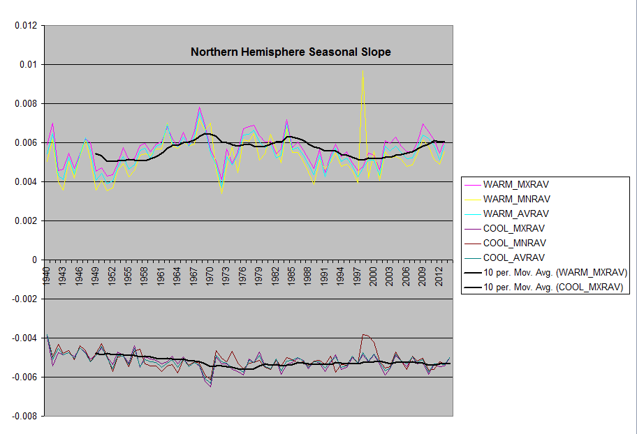


This is the average of the weather stations for each hemisphere.
Units are degrees F/day change.
Here I added calculated solar, by lat bands
This last one shows the step in temp after the 97-98 El Nino.
micro6500,
“I don’t think this is correct at all. First I show that only a small fraction even remains over a single night”
Yes, diurnal change could appear this way, except that its the mean that slowly adjusts to incremental CO2, not the p-p daily variability which is variability around that mean. Of course, half of the effect from CO2 emissions over the last 12 months is an imperceptible small fraction of a degree and in grand scheme of things is so deeply buried in the noise of natural variability it can’t be measured.
bits…
One other thing to notice is that the form of the response is exactly as expected from the DE,
Pi(t) = Po(t) + dE(t)/dt
where the EnergyFlux variable is dE/dt
Bits, if you haven’t yet, follow my name here, and read through the stuff there. It fits nicely with you question. And I have a ton of surface reports at the sourceforge link.
thanks well look at source forge!
George I would love to work with these data sets to validate the model (or not, right?) I looked at a bunch of the plots at http://www.palisad.com/co2/sens/ which is you, I assume.
bits…,
Yes, those are my plots. They’re a bit out of date (generated back in 2013) where since then, I’ve refined some of the derived variables including the time constants and added more data as it becomes available from ISCCP, but since the results aren’t noticeably different, I haven’t bothered to update the site. The D2 data from ISCCP does a lot of the monthly aggregation for you, is available on-line via the ISCCP web site and is a relatively small data set. It’s also reasonably well documented on the site (several papers by Rossow et. all). I’ve also obtained the DX data to do the aggregation myself after correcting the satellite cross calibration issues, but this is almost 1 Tb of data and hard to work with. Even with Google’s high speed Internet connections (back when I worked for them), it took me quite a while to download all of the data. I have observed that the D2 aggregation is relatively accurate, so I would suggest starting there.
One cannot cross validate the model as no statistical population underlies this model and a statistical population is required for cross validation.
terry,
“One cannot cross validate the model as no statistical population underlies this model and a statistical population is required for cross validation.”
3 decades of data sampled at 4 hour intervals, which for the most part is measured by 2 or more satellites, spanning the entire surface of the Earth at no more than a 30 km resolution is not enough of a statistical population?
The entity that you describe is a time series rather than a statistical population. Using a time series one can conduct an IPCC-style “evaluation.” One cannot conduct a cross validation as to so requires a statistical population and there isn’t one. Ten or more years ago, IPCC climatologists routinely confused “evaluation” with “cross validation.” The majority of journalists and university press agents still do so but today most professional climatologists make the distinction. To make the distinction is important because models that can be cross validated and models that can be evaluated differ in fundamental ways. Models that can be cross validated make predictions but models that can be evaluated make projections. Models that make predictions supply us with information about the outcomes of events but models that make projections supply us with no information. Models that make predictions are falsifiable but models that make projections are not falsifiable. A model that makes predictions is potentially usable in regulating Earth’s climate but not a model that makes projections. Professional climatologists should be building models that make predictions but they persist in building models that make projections for reasons that are unknown to me. Perhaps, like many amateurs, they are prone to confusing a time series with a statistical population.
Terry,
A statistical population is necessary when dealing with sparse measurements homogenized and extrapolated to the whole, as is the case with nearly all analysis done by consensus climate science. In fact a predicate to homogenization is a normal population of sites, which is never actually true (cherry picked sites are not a normal distribution). I’m dealing with the the antitheses of sparse, cherry picked data, moreover; more than a dozen different satellites with different sensors have accumulated data with overlapping measurements from at least 2 satellites looking a the same points on the surface at nearly the same time in just about all cases. Most measurements are redundant across 3 different satellites and many are redundant across 4 (two overlapping geosynchronous satellites and 2 polar orbiters at a much lower altitude).
If you’re talking about a statistical population being the analysis of the climate on many different worlds, we can point to the Moon and Mars as obeying the same laws, which they do. Venus is a little different due to the runaway cloud coverage condition dictating a completely different class of topology, none the less, it must still obeys the same laws of physics.
If neither of these is the case, you need to be much clearer about what in your mind constitutes a statistical population and why is this necessary to validate conformance to physical laws?
I’m not aware of past research in the field of global warming climatology. If you know of one please provide a citation.
“I’m not aware of past research in the field of global warming climatology. If you know of one please provide a citation.”
Hansen Lebedeff Homogenization
http://pubs.giss.nasa.gov/abs/ha00700d.html
GISStemp
http://pubs.giss.nasa.gov/abs/ha01700z.html
and any other temperature reconstruction that claims to support a high sensitivity or extraordinary warming trends.
co2isnotevil:
Thank you for positively responding to my request for a citation to a paper that made reference to a statistical population. In response to the pair of citations with which you responded, I searched the text of the paper that was cited first for terms that made reference to a statistical population. This paper was authored by the noted climatologist James Hansen.
The terms on which I searched were: statistical, population, sample, probability, frequency, relative frequency and temperature. “Statistical” produced no hits. “Population produced six hits, all of which were to populations of humans. “Sample” produced one hit which was, however, not to a collection of the elements of a statistical population.” “Probability” produced no hits. “Frequency” produced no hits. “Relative frequency” produced no hits. “Temperature” produced about 250 hits. Hansen’s focus was not upon a statistical population but rather was upon a temperature time series.
Terry,
The reference for the requirement for a normal distribution of sites is specific to Hansen Lebedeff homogenization. The second reference relies on this technique to generate the time series as do all other reconstructions based on surface measurements. My point was that the requirement for a normal distribution of sites is materially absent from the site selection used to reconstruct the time series in the second paper.
The term ‘statistical population’ is an overly general term, especially since statistical analysis underlies nearly everything about climate science, except the analysis of satellite data. Perhaps you can be more specific about how you define this term and offer an example as it relates to a field you are more familiar with.
co2isnotevil:
I agree with you regarding the over generality of the term “statistical population.” By “statistical population” I mean a defined set of concrete objects aka sampling units each of which is in a one-to-one relationship with a statistically independent unit event. For global warming climatology an element in this set can be defined by associating with the concrete Earth an element of a partition of the time line. Thus, under one of the many possible partitions, an element of this population is the concrete Earth in the period between Jan 1, 1900 at 0:00 hours GMT and Jan 1, 1930 at 0:00 hours GMT. Dating back to the beginning of the global temperature record in the year 1850 there are between 5 and 6 such sampling units. This number is too few by a factor of at least 30 for conclusions to be reached regarding the causes of rises in global temperatures over periods of 30 years.
I disagree with you when you state that “statistical analysis underlies nearly everything about climate science, except the analysis of satellite data.” I would replace “statistical” by “pseudostatistical” and “science” by “pseudoscience.”
Terry,
‘I would replace “statistical” by “pseudostatistical” and “science” by “pseudoscience.”’
Fair enough. So your point is that we don’t have enough history to ascertain trends, especially since there’s long term periodicity that’s not understood, and on that I agree which is why I make no attempt to establish the existence or non existence of trends. The analysis I’ve done is to determine the sensitivity by extracting a transfer function through quantifying the systems response to solar input from satellite measurements. The transfer function varies little from year to year, in fact, almost not at all, even day to day. It’s relatively static nature means that an extracted average will be statistically significant, especially since the number of specific samples is over 80K, where each sample is comprised of millions of individual measurements.
A key insight here is that dPower/dLattitude is well known from optics and geometry. dTemperature/dLattitude is also well known. To get dTemp/dPower just divide.
[The mods note that dPowerofdePope/dAltitude is likely to be directly proportional to the Qty_Angels/Distance. However, dTemperature/dAltitude seems to be inversely proportinal to depth as one gets hotter the further you are from dAngels. .mod]
Oops. I meant to say “I’m not aware of past research in the field of global warming climatology that was based upon a statistical population. If you know of one please provide a citation.
George / co2isnotevil
You have argued successfully in my view for the presence of a regulatory mechanism within the atmosphere which provides a physical constraint on climate sensitivity to internal thermal changes such as that from CO2
However, you seem to accept that the regulatory process fails to some degree such that CO2 retains a thermal effect albeit less than that proposed by the IPCC.
You have not explained how the regulatory mechanism could fail nor have you considered the logical consequences of such failure.
I have provided a mass based mechanism which purports to eliminate climate thermal sensitivity from CO2 or any other internal processes altogether but which acknowledges that as a trade off there must be some degree of internal circulation change that alters the balance between KE and PE in the atmosphere so that hydrostatic equilibrium can be retained.
That mechanism appears to be consistent with your findings.
If climate sensitivity to CO2 is not entirely eliminated then surface temperature must rise but then one has more energy at the surface than is required to both achieve radiative equilibrium with space AND provide the upward pressure gradient force that keeps the mass of the atmosphere suspended off the surface against the downward force of gravity yet not allowed to drift off to space.
The atmosphere must expand upwards to rebalance but that puts the new top layer in a position where the upward pressure gradient force exceeds the force of gravity so that top layer will be lost to space.
That reduces the mass and weight of the atmosphere so the higher surface temperature can again push the atmosphere higher to create another layer above the critical height so that the second new higher layer is lost as well.
And so it continues until there is no atmosphere.
The regulatory process that you have identified cannot be permitted to fail if the atmosphere is to be retained.
The gap between your red and green lines is the surface temperature enhancement created by conduction and convection.
The closeness of the curves of the red and green lines shows the regulatory process working perfectly with no failure.
George: In Figure 2, if A equals 0.75 – which makes OLR 240 W/m2 – then DLR is 144 W/m2 (Ps*A/2). This doesn’t agree with observations. Therefore your model is wrong.
(Some people believe DLR doesn’t exist or isn’t measured properly by the same kind of instruments used to measure TOA OLR. If DLR is in doubt, so is TOA OLR – in which case the whole post is meaningless.)
Frank,
Ps*A/2 is NOT a quantification of DLR, i.e the total amount of IR the atmosphere as a whole passes to the surface, but rather it’s the equivalent fraction of ‘A’ that is *effectively* gained back by the surface in the steady-state. Or it’s such that the flow of energy in and out of the whole system, i.e. the rates of joules gained and lost at the surface and TOA, would be the same. Nothing more.
It’s not a model or emulation of the actual thermodynamics and thermodynamic path manifesting the energy balance, for it would surely be spectacularly wrong if it were claimed to be.
RW: What BS! The arrow with Ps underneath is the flux leaving the surface of the Earth, 385 W/m2. The pair of arrows summing to P_o = Ps*(1-A/2) is TOA OLR flux, 240 W/m2. One arrow is the flux transmitted through the atmosphere, the other is the flux emitted upward by the atmosphere. The arrow back to the surface Ps*(A/2) must be DLR and it equals 144 W/m2 – at least as shown. Don’t tell me three of the arrows symbolize flues, but the fourth something different .. “effective gain”
You should be telling me that convection also carries heat from the surface to the atmosphere, so there is another 100 W/m2 that could be added to DLR. However, Doug arbitrary divided the absorbed flux from the surface (A) in half and sent half out the TOA and half to the surface. So, should we partition the heat provided by convection in the same way? Why? That will make TOA OLR wrong.
George,
Maybe we can clear this up. What does your RT simulation calculate for actual DLR at the surface? It’s roughly 300 W/m^2…maybe like 290 W/m^2 or something, right?
RW,
“Maybe we can clear this up. What does your RT simulation calculate for actual DLR at the surface?”
First of all, we need to remove non radiant power from the analysis. This is the zero sum influence of latent heat, convection and any other non radiant power leaving the surface and returned, whose effects are already accounted for by the temperature of the EQUIVALENT gray body emitter and which otherwise have no impact on the radiative balance. All non radiant flux does is to temporarily reorganize surface energy and while if may affect the specific origin of emitted energy, it has no influence on the requirements for what that emitted energy must be. Note that this is the case, even if some of the return of non radiant energy was actually returned as non radiant energy transformed into photons. However; there seems to be enough non radiant return (rain, weather, downdrafts, etc.) to account for the non radiant energy entering the atmosphere, most of which is latent heat.
When you only account for the return of surface emissions absorbed by GHG’s and clouds, the DLR returned to the surface is about 145 W/m^2. Remember that there are 240 W/m^2 coming from the Sun warming the system. In LTE, all of this can be considered to all affect the surface temperature owing to the short lifetime of atmospheric water which is the only significant component of the atmosphere that absorbs any solar input. Given that the surface and by extension the surface water temporarily lifted into the atmosphere absorbs 240 W/m^2, only 145 W/m^2 of DLR is REQUIRED to offset the 385 W/m^2 of surface emissions consequential to its temperature. If there was more actual DLR this, the surface temperature would be far higher then it is.
Measurements of DLR are highly suspect owing to the omnidirectional nature of atmospheric photons and interference from the energy of molecules in motion, so if anyone thinks they are measuring 300 W/m^2 or more DLR, there’s a serious flaw in their measurement methodology, which I expect would be blindly accepted owing to nothing more than confirmation bias where they want to see a massive amount of DLR to make the GHG effect seem much more important than it actually is.
Frank,
“RW: What BS! The arrow with Ps underneath is the flux leaving the surface of the Earth, 385 W/m2. The pair of arrows summing to P_o = Ps*(1-A/2) is TOA OLR flux, 240 W/m2. One arrow is the flux transmitted through the atmosphere, the other is the flux emitted upward by the atmosphere. The arrow back to the surface Ps*(A/2) must be DLR and it equals 144 W/m2 – at least as shown. Don’t tell me three of the arrows symbolize flues, but the fourth something different .. “effective gain”
You should be telling me that convection also carries heat from the surface to the atmosphere, so there is another 100 W/m2 that could be added to DLR. However, Doug arbitrary divided the absorbed flux from the surface (A) in half and sent half out the TOA and half to the surface. So, should we partition the heat provided by convection in the same way? Why? That will make TOA OLR wrong.
If Ps*(A/2) were a model of the actual physics, i.e. actual thermodynamics occurring, then yes it would be spectacularly wrong (or BS as you say). But it’s only an abstraction or an *equivalent* derived black box model so far as quantifying the aggregate behavior of the thermodynamics and thermodynamic path manifesting the balance.
Let me ask you this question. What does DLR at the surface tell us so far as how much of A (from the surface) ultimately contributes to or is ultimately driving enhanced surface warming? It doesn’t tell us anything at all, much less quantify its effect on ultimate surface warming among all the other physics occurring all around it. Right?
BTW, the only way to accurately measure DLR is with a LWIR specific sensor placed at the bottom of a tall vacuum bottle (tube) pointed up. The apparatus should be placed on the surface and insulated on all sides except the top. In other words, you must measure ONLY those photons directed perpendicular to the surface and you must isolate the sensor from thermal contamination from omnidirectional GHG emissions and the kinetic energy of particles in motion.
“..then DLR is 144 W/m2 (Ps*A/2). This doesn’t agree with observations. Therefore your model is wrong.”
No, Fig. 2 model is a correct text book physics analogue. What is wrong is setting A=0.75 too “dry” when global observations show A is closer to = 0.8 which calculates Fig. 2 global atm. gray block DLR of 158 (not 144 which is too low). Then after TFK09 superposing thermals (17) and evapotranspiration (80) with solar SW absorbed (78) by the real atm. results 158+17+80+78=333 all sky emission to surface over the ~4 years 2000-2004.
Trick,
The value A can be anythin and if it is 0.8 then more than 50% of absorption must be emitted into space and less than half is required to be returned to the surface. I’m not saying that this is impossible, but goes counter to the idea that more tha half must be returned to the surface. Keep in mind that the non radiant fluxes are not a component of A or of net surface emissions.
”BTW, the only way to accurately measure DLR is with a LWIR specific sensor placed at the bottom of a tall vacuum bottle (tube) pointed up…. you must measure ONLY those photons directed perpendicular to the surface“
No, the flux through the bottom of the atm. unit area column arrives from a hemisphere of directions looking up and down. The NOAA surface and CERES at TOA radiometers admit viewed radiation from all the angles observed.
“Keep in mind that the non radiant fluxes are not a component of A or of net surface emissions”
They are in the real world from which global A=0.8 is measured and calculated to 290.7K global surface temperature using your Fig. 2 analogue.
“if it is 0.8 then more than 50% of absorption must be emitted into space and less than half is required to be returned to the surface.”
The 0.8 global measured atm. Fig. 2 A emissivity returns (emits) half (158) to the surface and emits half (158) to space as in TFK09 balance real world observed Mar 2000 to May 2004: 158+78+80+17=333 all sky emission to surface and 158+41+40= 239 all-sky to space + 1 absorbed = 240, rounded. Your A=0.75 does not balance to real global world observed, though it might be result of a local RT balance as you write.
Phil,
“The collisions do not induce emission of a photon they cause a transfer of kinetic energy to the colliding partner …”
The mechanism of collisional broadening, which supports the exchange between state energy and translational kinetic energy, converts only small amounts at a time and in roughly equal amounts on either side of resonance and in both directions.
The kinetic energy of an O2/N2 molecule in motion is about the same as the energy of a typical LWIR photon. The velocity of the colliding molecule can not drop down to or below zero to energize a GHG, nor will its kinetic energy double upon a collision. Beside, any net conversion of GHG absorption to the translational kinetic energy of N2/O2 is no longer available to contribute to the radiative balance of the planet as molecules in motion do not radiate significant energy, unless they are GHG active.
When we observe the emitted spectrum of the planet from space, there’s far too much energy in the absorption bands to support your hypothesis. Emissions are only attenuated by only about 50%, where if GHG absorption was ‘thermalized’ in the manner you suggest, it would be redistributed across the rest of the spectrum and we would not only see far less in the absorption bands, we would see more in the transparent window and the relative attenuation would be an order of magnitude or more.
co2isnotevil said:
1) “First of all, we need to remove non radiant power from the analysis. This is the zero sum influence of latent heat, convection and any other non radiant power leaving the surface and returned, whose effects are already accounted for by the temperature of the EQUIVALENT gray body emitter and which otherwise have no impact on the radiative balance. All non radiant flux does is to temporarily reorganize surface energy and while if may affect the specific origin of emitted energy, it has no influence on the requirements for what that emitted energy must be”
Excellent. In other words just what I have been saying about the non radiative energy tied up in convective overturning.
The thing is that such zero sum non radiative energy MUST be treated as a separate entity from the radiative exchange with space yet it nonetheless contributes to surface heating which is why we have a surface temperature 33K above S-B.
Since trhose non radiative elements within the system are derived from the entire mass of the atmosphere the consequence of any radiative imbalance from GHGs is too trivial to consider and in any event can be neutralised by circulation adjustments within the mass of the atmosphere.
AGW proponents simply ignore such energy being returned to the surface and therefore have to propose DWIR of the same power to balance the energy budget.
In reality such DWIR as there is has already been taken into account in arriving at the observed surface temperature so adding an additional amount (in place of the correct energy value of non radiative returning energy) is double counting.
2) “All non radiant flux does is to temporarily reorganize surface energy and while if may affect the specific origin of emitted energy it has no influence on the requirements for what that emitted energy must be”
Absolutely. The non radiative flux can affect the balance of energy emitted from the surface relative to emissions from within the atmosphere and it is variable convective overturning that can swap emissions between the two origins so as to maintain hydrostatic equilbrium. The medium of exchange is KE to PE in ascent and PE to KE in descent.
The non radiative flux itself has no influence on the requirement for what that emitted energy must be BUT it does provide a means whereby the requirement can be consistently met even in the face of imbalances created by GHGs.
George is so close to having it all figured out.
CO2isnotevil writes above and is endorsed by Wilde: “First of all, we need to remove non radiant power from the analysis. This is the zero sum influence of latent heat, convection and any other non radiant power leaving the surface and returned, whose effects are already accounted for by the temperature of the EQUIVALENT gray body emitter and which otherwise have no impact on the radiative balance. All non radiant flux does is to temporarily reorganize surface energy and while if may affect the specific origin of emitted energy, it has no influence on the requirements for what that emitted energy must be. ”
This is ridiculous. Let’s take the lapse rate, which is produced by convection. It controls the temperature (and humidity) within the troposphere, where most photons that escape to space are emitted (even in your Figure 2). Let’s pick a layer of atmosphere 5 km above the surface at 288 K where the current lapse rate (-6.5 K/km, technically I shouldn’t use the minus sign) means the temperate is 255 K. If we change the lapse rate to DALR (-10 K/km) or to 0 K/m – to make extreme changes to illustrate my point – the temperature will be 238 K or 288 K. Emission from 5 km above the surface, which varies with temperature, is going to be very different if the lapse rate changes. If you think terms of T^4, which is an oversimplification, 238 K is about 28% reduction in emission and 288 K is about 50% increase in emission. At 10 km, these differences will be twice as big. And this WILL change how much radiation comes out of the TOA. Absorption is fairly independent of temperature, so A in Figure 2 won’t change much.
By removing these internal transfers of heat, you disconnect surface temperature from the temperature of the GHGs that are responsible for emitting photons that escape to space – that radiatively cool the earth. However, their absorption is independent of temperature. You think TOA OLR is the result of an emissivity that can be calculated from absorption. Emission/emissivity is controlled by temperature variation within the atmosphere, not absorption or surface temperature.
If our atmosphere didn’t have a lapse rate, the GHE would be zero!
In the stratosphere, where temperature increase with altitude, increasing CO2 increases radiative cooling to space and cools the stratosphere. Unfortunately, the change is small because few photons escaping to space originate there.
CO2isnotevil writes: “When you only account for the return of surface emissions absorbed by GHG’s and clouds, the DLR returned to the surface is about 145 W/m^2. Remember that there are 240 W/m^2 coming from the Sun warming the system.”
Partially correct. The atmosphere can emit an average of 333 W/m2 of DLR, not 145 W/m2 as calculated, because it receives about 100 W/m2 of latent and sensible heat from convection and absorbs about 80 W/m2 of SWR (that isn’t reflected to space and doesn’t reach the surface). Surface temperature is also the net result of all incoming and outgoing fluxes. ALL fluxes are important – you end up with nonsense by ignoring some and paying attention to others.
CO2isnotevil writes; “In LTE, all of this can be considered to all affect the surface temperature owing to the short lifetime of atmospheric water which is the only significant component of the atmosphere that absorbs any solar input.”
Read Grant Petty’s book for meteorologists, “A First Course in Atmospheric Radiation” and learn what LTE means. The atmosphere is not in thermodynamic equilibrium with the radiation passing through it. If it were, we would observe a smooth blackbody spectrum of emission intensity, perhaps uniformly reduced by emissivity. However, we observe a jagged spectrum with very different amounts of radiation arriving at adjacent wavelengths (where the absorption of GHGs differs). LTE means that the emission by GHGs in the atmosphere depends only on the local temperature (through B(lambda,T)) – and not equilibrium with the local radiation field. It means that excited states are created and relaxed by collisions much faster than by absorption or emission of photons – that a Boltzmann distribution of excited and ground states exists. See
CO2isnotevil writes: “Measurements of DLR are highly suspect owing to the omnidirectional nature of atmospheric photons and interference from the energy of molecules in motion, so if anyone thinks they are measuring 300 W/m^2 or more DLR, there’s a serious flaw in their measurement methodology, which I expect would be blindly accepted owing to nothing more than confirmation bias where they want to see a massive amount of DLR to make the GHG effect seem much more important than it actually is.”
In that case, all measurements of radiation are suspect. All detectors have a “viewing angle”, including those on CERES which measure TOA OLR and those here on Earth which measure emission of thermal infrared. We live and make measurements of thermal IR surrounded by a sea of thermal infrared photons. Either we know how to deal with the problem correctly and can calibrate one instrument using another or we know nothing and are wasting our time. DLR has been measured with instruments that record the whole spectrum in addition to pyrometers. I’ll refer you to figure’s in Grant Petty’s book showing the spectrum of DLR. You can’t have it both ways. You can’t cherry-pick TOA OLR and say that value is useful and at DLR and say that value may be way off. That reflects your confirmation bias in favor or a model that can’t explain what we observe.
“BTW, the only way to accurately measure DLR is with a LWIR specific sensor placed at the bottom of a tall vacuum bottle (tube) pointed up. The apparatus should be placed on the surface and insulated on all sides except the top. In other words, you must measure ONLY those photons directed perpendicular to the surface and you must isolate the sensor from thermal contamination from omnidirectional GHG emissions and the kinetic energy of particles in motion.”
Right, but the RT simulations don’t rely on sensors to calculate DLR. Doesn’t your RT simulation get around 300 W/m^2? The 3.6 W/m^2 of net absorption increase per 2xCO2 — you’re RT simulations quantify this the same as everyone else in the field, i.e. the difference between the reduced IR intensity at the TOA and the increased IR intensity at the surface (calculated via the Schwartzchild eqn. the same way everyone else does). This result is not possible without the manifestation of a lapse rate, i.e. decreasing IR emission with height.
You need to clarify that your claimed Ps*A/2 is only an abstraction, i.e. only an equivalent quantification of DLR after you’ve subtracted the 240 W/m^2 entering from the Sun from the required net flux gained at the surface required to replace the 385 W/m^2 radiated away a consequent of its temperature. And that it’s only equivalent so far as quantifying the aggregate behavior of the system, i.e. the rates of joules gained and lost at the TOA.
People like Frank here:
https://wattsupwiththat.com/2017/01/05/physical-constraints-on-the-climate-sensitivity/comment-page-1/#comment-2395000
are getting totally faked out by all of this, i.e. what you’re doing. You need to explain and clarify that what you’re modeling here isn’t the actual thermodynamics and thermodynamic path manifesting the energy balance. Frank (and many others I’m sure) think that’s what you’re doing here. When you’re talking equivalence, it would be helpful to stipulate it, because it’s not second nature to everyone as it is for you.
George,
My understanding is your equivalent model isn’t saying anything at all about the actual amount of DLR, i.e. the actual amount of IR flux the atmosphere as a whole passes to the surface. It’s not attempting to quantify the actual downward IR intensity at the surface/atmosphere boundary. Most everyone, including especially Frank, think that’s what you’re claiming with your model. It isn’t, and you need to explain and clarify this.
The surface of the planet only emits a NET of 385 W/m^2 consequential to its temperature. Latent heat and thermals are not emitted, but represents a zero sum from an energy perspective since any effect the round trip path that energy takes has is already accounted for by the average surface temperature. The surface requires 385 W/m^2 of input to offset the 385 W/m^2 being emitted.
The transport of energy by matter is an orthogonal transport path to the photon transport related to the sensitivity, and the ONLY purpose of this analysis was to quantify the relationship between the surface whose temperature we care about (the surface emitting 385 W/m^2) and the outer boundary of the planet which is emitting 240 W/m^2. The IPCC defines the incremental relationship between these two values as the sensitivity. My analysis quantifies this relationship with a model and compares the model to the data that the model is representing. Since the LTE data matches the extracted transfer function (SB with an emissivity of 0.62), the sensitivity of the model represents the sensitivity measured by the data so closely, the minor differences are hardly worth talking about.
The claim for the requirement of 333 W/m^2 of DLR comes from Trenberth’s unrepresentative energy balance, but this has NEVER been measured properly, even locally, as far as I can tell, and nowhere is there any kind of justification, other then Trenberth’s misleading balance, that 333 W/m^2 is a global average.
The nominal value of A=0.75 is within experimental error of what you get from line by line analysis of the standard atmosphere with nominal clouds (clouds being the most important consideration). Half of this is required both to achieve balance at the top boundary and to achieve balance at the bottom boundary.
The real problem is that too many people are bamboozled by all the excess complexity added to make to climate system seem more complex than it needs to be. The problem is that the region between the 2 characterized boundaries is very complex and full of unknowns and you will never get any simulation or rationalization about its behavior correct until you understand how it MUST behave at its boundaries.