Guest Post by Willis Eschenbach
One of the best parts of writing for the web is the outstanding advice and guidance I get from folks with lots of experience. I recently had the good fortune to have Robert Brown of Duke University recommend a study by Demetris Koutsoyiannis entitled The Hurst phenomenon and fractional Gaussian noise made easy. It is indeed “made easy”, I recommend it strongly. In addition, Leif Svalgaard recommended another much earlier study of a similar question (using very different terminology) in a section entitled “Random series, and series with conservation” of a book entitled “Geomagnetism“. See p.584, and Equation 91. While it is not “made hard”, it is not “made easy” either.
Between these two excellent references, I’ve come to a much better understanding of the Hurst phenomenon and of fractional gaussian noise. In addition, I think I’ve come up with a way to calculate the equivalent number of independent data points in an autocorrelated dataset.
So as I did in my last post on this subject, let me start with a question. Here is the recording of the Nile River levels made at the “Roda Nilometer” on the Nile River. It is one of the longest continuous climate-related records on the planet, extending from the year 622 to the year 1284, an unbroken stretch of 633 years. There’s a good description of the nilometer here, and the nilometer dataset is available here.
 Figure 1. The annual minimum river levels in Cairo, Egypt as measured by the nilometer on Roda Island.
So without further ado, here’s the question:
Is there a significant trend in the Nile River over that half-millennium plus from 622 to 1284?
Well, it sure looks like there is a trend. And a standard statistical analysis says it is definitely significant, viz:
Coefficients:

                 Estimate Std.      Error t value P-value less than

(Intercept)          1.108e+03  6.672e+00 166.128  < 2e-16 ***

seq_along(nilometer) 1.197e-01  1.741e-02   6.876 1.42e-11 ***

---

Signif. codes:  0 ‘***’ 0.001 ‘**’ 0.01 ‘*’ 0.05 ‘.’ 0.1 ‘ ' 1

Residual standard error: 85.8 on 661 degrees of freedom

Multiple R-squared:  0.06676, Adjusted R-squared:  0.06535

F-statistic: 47.29 on 1 and 661 DF,  p-value: 1.423e-11
That says that the odds of finding such a trend by random chance are one in 142 TRILLION (p-value less than 1.42e-11).
Now, due to modern computer speeds, we don’t have to take the statisticians’ word for it. We can actually run the experiment ourselves. It’s called the “Monte Carlo” method. To use the Monte Carlo method, we generate say a thousand sets (instances) of 663 random numbers. Then we measure the trends in each of the thousand instances, and we see how the Nilometer trend compares to the trends in the pseudodata. Figure 2 shows the result:
 Figure 2. Histogram showing the distribution of the linear trends in 1000 instances of random normal pseudodata of length 633. The mean and standard deviation of the pseudodata have been set to the mean and standard deviation of the nilometer data.
As you can see, our Monte Carlo simulation of the situation agrees completely with the statistical analysis—such a trend is extremely unlikely to have occurred by random chance.
So what’s wrong with this picture? Let me show you another picture to explain what’s wrong. Here are twenty of the one thousand instances of random normal pseudodata … with one of them replaced by the nilometer data. See if you can spot which one is nilometer data just by the shapes:
 Figure 3. Twenty random normal sets of pseudodata, with one of them replaced by the nilometer data.
If you said “Series 7 is nilometer data”, you win the Kewpie doll. It’s obvious that it is very different from the random normal datasets. As Koutsoyiannis explains in his paper, this is because the nilometer data exhibits what is called the “Hurst phenomenon”. It shows autocorrelation, where one data point is partially dependent on previous data points, on both long and short time scales. Koutsoyiannis shows that the nilometer dataset can be modeled as an example of what is called “fractional Gaussian noise”.
This means that instead of using random normal pseudodata, what I should have been using is random fractional Gaussian pseudodata. So I did that. Here is another comparison of the nilometer data, this time with 19 instances of fractional Gaussian pseudodata. Again, see if you can spot the nilometer data.
 Figure 4. Twenty random fractional Gaussian sets of pseudodata, with one of them replaced by the nilometer data.
Not so easy this time, is it, they all look quite similar … the answer is Series 20. And you can see how much more “trendy” this kind of data is.
Now, an internally correlated dataset like the nilometer data is characterized by something called the “Hurst Exponent”, which varies from 0.0 to 1.0. For perfectly random normal data the Hurst Exponent is 0.5. If the Hurst Exponent is larger than that, then the dataset is positively correlated with itself internally. If the Hurst Exponent is less than 0.5, then the dataset is negatively correlated with itself. The nilometer data, for example, has a Hurst Exponent of 0.85, indicating that the Hurst phenomenon is strong in this one …
So what do we find when we look at the trends of the fractional Gaussian pseudodata shown in Figure 4? Figure 5 shows an overlay of the random normal trend results from Figure 2, displayed on top of the fractional Gaussian trend results from the data exemplified in Figure 4.
 Figure 5. Two histograms. The blue histogram shows the distribution of the linear trends in 1000 instances of random fractional Gaussian pseudodata of length 633. The average Hurst Exponent of the pseudodata is 0.82 That blue histogram is overlaid with a histogram in red showing the distribution of the linear trends in 1000 instances of random normal pseudodata of length 633 as shown in Figure 2. The mean and standard deviation of the pseudodata have been set to the mean and standard deviation of the nilometer data.
I must admit, I was quite surprised when I saw Figure 5. I was expecting a difference in the distribution of the trends of the two sets of pseudodata, but nothing like that … as you can see, while standard statistics says that the nilometer trend is highly unusual, in fact, it is not unusual at all. About 15% of the pseudodata instances have trends larger than that of the nilometer.
So we now have the answer to the question I posed above. I asked whether there was a significant rise in the Nile from the year 622 to the year 1284 (see Figure 1). Despite standard statistics saying most definitely yes, amazingly, the answer seems to be … most definitely we don’t know. The trend is not statistically significant. That amount of trend in a six-century-plus dataset is not enough to say that it is more than just a 663-year random fluctuation of the Nile. The problem is simple—these kinds of trends are common in fractional Gaussian data.
Now, one way to understand this apparent conundrum is that because the nilometer dataset is internally correlated on both the short and long term, it is as though there were fewer data points than the nominal 633. The important concept is that since the data points are NOT independent of each other, a large number of inter-dependent data points acts statistically like a smaller number of truly independent data points. This is the basis of the idea of the “effective n”, which is how such autocorrelation issues are often handled. In an autocorrelated dataset, the “effective n”, which is the number of effective independent data points, is always smaller than the true n, which is the count of the actual data.
But just how much smaller is the effective n than the actual n? Well, there we run into a problem. We have heuristic methods to estimate it, but they are just estimations based on experience, without theoretical underpinnings. I’ve often used the method of Nychka, which estimates the effective n from the lag-1 auto-correlation (Details below in Notes). The Nychka method estimates the effective n of the nilometer data as 182 effective independent data points … but is that correct? I think that now I can answer that question, but there will of course be a digression.
I learned two new and most interesting things from the two papers recommended to me by Drs. Brown and Svalgaard. The first was that we can estimate the number of effective independent data points from the rate at which the standard error of the mean decreases with increasing sample size. Here’s the relevant quote from the book recommended by Dr. Svalgaard:
 Figure 6. See the paper for derivation and details. The variable “m” is the standard deviation of the full dataset. The function “m(h)” is the standard deviation of the means of the full dataset taken h data points at a time.
Now, you’ve got to translate the old-school terminology, but the math doesn’t change. This passage points to a method, albeit a very complex method, of relating what he calls the “degree of conservation” to the number of degrees of freedom, which he calls the “effective number of random ordinates”. I’d never thought of determining the effective n in the manner he describes.
This new way of looking at the calculation of neff was soon complemented by what I learned from the Koutsoyiannis paper recommended by Dr. Brown. I found out that there is an alternative formulation of the Hurst Exponent. Rather than relating the Hurst Exponent to the range divided by the standard deviation, he shows that the Hurst Exponent can be calculated as a function of the slope of the decline of the standard deviation with increasing n (the number of data points). Here is the novel part of the Koutsoyiannis paper for me:
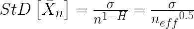
 Figure 7. The left-hand side of the equation is the standard deviation of the means of all subsets of length “n”, that is to say, the standard error of the mean for that data. On the right side, sigma ( σ ), the standard deviation of the means, is divided by “n”, the number of data points, to the power of (1-H), where H is the Hurst Exponent. See the paper for derivation and details.
In the statistics of normally distributed data, the standard error of the mean (SEM) is sigma (the standard deviation of the data) divided by the square root of N, the number of data points. However, as Koutsoyiannis shows, this is a specific example of a more general rule. Rather than varying as a function of 1 over the square root of n (n^0.5), the SEM varies as 1 over n^(1-H), where H is the Hurst exponent. For a normal dataset, H = 0.5, so the equation reduces to the usual form.
SO … combining what I learned from the two papers, I realized that I could use the Koutsoyiannis equation shown just above to estimate the effective n. You see, all we have to do is relate the SEM shown above, 

where the left-hand term is the standard error of the mean, and the two right-hand expressions are different equivalent ways of calculating that same standard error of the mean.
By inverting the fractions, canceling out the sigmas, and squaring both sides we get

Egads, what a lovely result! Equation 1 calculates the number of effective independent data points using only n, the number of datapoints in the dataset, and H, the Hurst Exponent.
As you can imagine, I was quite interested in this discovery. However, I soon ran into the next oddity. You may recall from above that using the method of Nychka for estimating the effective n, we got an effective n (neff) of 182 independent data points in the nilometer data. But the Hurst Exponent for the nilometer data is 0.85. Using Equation 1, this gives us an effective n of 663^(2-2* 0.85) equals seven measly independent data points. And for the fractional Gaussian pseudodata, with an average Hurst Exponent of 0.82, this gives only about eleven independent data points.
So which one is right—the Nychka estimate of 182 effective independent datapoints, or the much smaller value of 11 calculated with Equation 1? Fortunately, we can use the Monte Carlo method again. Instead of using 663 random normal data points stretching from the year 622 to 1284, we can use a smaller number like 182 datapoints, or even a much smaller number like 11 datapoints covering the same time period. Here are those results:
 Figure 8. Four histograms. The solid blue filled histogram shows the distribution of the linear trends in 1000 instances of random fractional gaussian pseudodata of length 633. The average Hurst Exponent of the pseudodata is 0.82 That blue histogram is overlaid with a histogram in red showing the distribution of the linear trends in 1000 instances of random normal pseudodata of length 633. These two are exactly as shown in Figure 2. In addition, the histograms of the trends of 1000 instances of random normal pseudodata of length n=182 and n=11 are shown in blue and black. Mean and standard deviation of the pseudodata has been set to the mean and standard deviation of the nilometer data.
I see this as a strong confirmation of this method of calculating the number of equivalent independent data points. The distribution of the trends with 11 points of random normal pseudodata is very similar to the distribution of the trends with 663 points of fractional Gaussian pseudodata with a Hurst Exponent of 0.82, exactly as Equation 1 predicts.
However, this all raises some unsettling questions. The main issue is that the nilometer data is by no means the only dataset out there that exhibits the Hurst Phenomena. As Koutsoyiannis observes:
The Hurst or scaling behaviour has been found to be omnipresent in several long time series from hydrological, geophysical, technological and socio-economic processes. Thus, it seems that in real world processes this behaviour is the rule rather than the exception. The omnipresence can be explained based either on dynamical systems with changing parameters (Koutsoyiannis, 2005b) or on the principle of maximum entropy applied to stochastic processes at all time scales simultaneously (Koutsoyiannis, 2005a).
As one example among many, the HadCRUT4 global average surface temperature data has an even higher Hurst Exponent than the nilometer data, at 0.94. This makes sense because the global temperature data is heavily averaged over both space and time. As a consequence the Hurst Exponent is high. And with such a high Hurst Exponent, despite there being 1,977 months of data in the dataset, the relationship shown above indicates that the effective n is tiny—there are only the equivalent of about four independent datapoints in the whole of the HadCRUT4 global average temperature dataset. Four.
SO … does this mean that we have been chasing a chimera? Are the trends that we have believed to be so significant simply the typical meanderings of high Hurst Exponent systems? Or have I made some foolish mistake?
I’m up for any suggestions on this one …
Best regards to all, it’s ten to one in the morning, full moon is tomorrow, I’m going outside for some moon viewing …
w.
UPDATE: Demetris Koutsoyiannis was kind enough to comment below. In particular, he said that my analysis was correct. He also pointed out in a most gracious manner that he was the original describer of the relationship between H and effective N, back in 2007. My thanks to him.
Demetris Koutsoyiannis July 1, 2015 at 2:04 pm
Willis, thank you very much for the excellent post and your reference to my work. I confirm your result on the effective sample size — see also equation (6) in
http://www.itia.ntua.gr/en/docinfo/781/
As You Might Have Heard: If you disagree with someone, please have the courtesy to quote the exact words you disagree with so we can all understand just exactly what you are objecting to.
The Data Notes Say:
### Nile river minima
###
## Yearly minimal water levels of the Nile river for the years 622
## to 1281, measured at the Roda gauge near Cairo (Tousson, 1925,
## p. 366-385). The data are listed in chronological sequence by row.
## The original Nile river data supplied by Beran only contained only
## 500 observations (622 to 1121). However, the book claimed to have
## 660 observations (622 to 1281). I added the remaining observations
## from the book, by hand, and still came up short with only 653
## observations (622 to 1264).
### — now have 663 observations : years 622–1284 (as in orig. source)
The Method Of Nychka: He calculates the effective n as follows:

where “r” is the lag-1 autocorrelation.
Excellent article Willis and of course thanks to RGB and Dr S for the core material.
It is not surprising that temperature data is strongly auto correlated since the thermal inertia ensure it has to be. HadCruft$ [sic] is a bastard mix of incompatible data. IMO it should be completely ignored when doing anything about the physics of climate.
It would be more relevant to look at land and sea separately. I would expect SST to be more strongly autocorrelated than land SAT.
This simple AR1 behaviour can be removed by taking the first difference ( dT/dt ). This is also the immediate effect of an imbalance in radiative ‘forcing’.
It may be more interesting to see how many separate points you get from that.
This seems to echo the argument Doug Keanan was having with the Met Office ( that ended up in the House of Lords ) about what the relevant statistical model was to apply to the data when making estimations of significance of global warming. AFAIR he used a different model and showed the change was not significant.
I’ve been saying for years that this obsession with “trends” is meaningless and simply reflects the technical limitations of those so keen drawing straight lines through everything they find, with the naive belief that a “trend” is some inherent property which reveals the true nature of everything.
You point about processing is also a good one. How do the Hurst exponents differ for ICOADS SST and HadSST3 ( since 1946 when SST has been more consistently measured )?
A question that I think needs to be asked:
If the volume of water that flows down the Nile River each year is measured by the height of the water each year over the span of 633 years then the comparison of annual water flows would only work if there was no changes in the river.
But over the span of 633 years I think it would be unreasonable to think there would be no changes in the river and hence accurate comparisons of water flows as measured by heights of the water level would be questionable.
Remember this time series only records the year’s low point of the river. It says nothing about most of the year and nothing about flood.
On a guided tour of Zion National Park, the guide informed us that the puny little river in the bottom of the canyon is a raging torrent in the spring melt such that 99% of the year’s flow is accounted for in just a couple of days.
Reality.
Combotechie
The data could also be showing that the Nile is silting up. That could be tested: if it is high one year (a peak flow cleans out silt) is it always lower the next? Is there a slow rise then a peak that lowers the river bed ‘suddenly’? How about three high years in a row? It is a river, after all.
If there is a 2 ft rise over 6 centuries, the silting effect and a 1470 weather year cycle could easily produce it. The importance of your point is that one has to consider the system being examined, not just the numbers. Viewing the flood height as only caused by rainfall and therefore flow volume is to ignore the fact it is a river and that there is a ‘Nile Delta’ for a very good reason. Flood height at the measurement height could be dominated by the shifting sand bars downstream.
Very interesting phenomenon to analyse.
The four effective data points of global SST:
1915,1934,1975,1995
next effective data point 1919. 😉
those are inflection pts. Assume you meant 2019 for the next.
Oh dear earlier post went AWOL.
Basically: great article Willis.
HadCruft4 is a meaningless mix of incompatible data, irrelevant to any physical study.
How about doing same thing on first difference ( dT/dt ) to remove the obvious autocorrelation SST.
cf H for icoads SST and hadSST3 since 1946 ?
excellent exploration!
While I have major issues with the statistical assumptions necessary to deal inferentially with these data, I wonder if anyone does a-priori power analysis anymore? Could help with imagining effective n, but won’t alleviate the auto-correlation problem –
http://effectsizefaq.com/2010/05/31/what-is-statistical-power/
previous post probably in bit bin due to use of the B word. Which was used as a cuss word to indicate the illegitimate intermarriage of land and sea data.
Did you imply that the land and sea data’s parents were not married?
A very nice post, Willis.
Some time ago, ca. 2008, with assistance from Tomas Milanovic and a brief exchange with Demitris Koutsoyiannis, I did a few Hurst coefficient analyses of (1) the original Lorenz 1963 equation system, (2) some data from the physical domain, and (3) some calculated temperature results from a GCM. In the second file, I gave a review of the results presented in the first file; probably too much review. The errors in the content of the files are all mine.
The second file has the Hurst coefficient results for the monthly average Central England Temperature (CET). I said I would get to the daily average for the CET record, but I haven’t yet.
The Lorenz system results, pure temporal chaotic response, showed that for many short periods the Hurst exponent has more or less H = 1.0. For intermediate period lengths the exponent was H = 0.652, and for fewer and longer periods the exponent was H = 0.50.
I found some temperature data for January in Sweden that covered the years 1802 to 2002. The exponent was about 0.659. The monthly-average CET record gave H = 0.665. A version of the HadCRUT yearly-mean GMST data gave H = 0.934 for a 160 year data set.
I got some 440 years of monthly-average GCM results for January from the Climate Explorer site:
# using minimal fraction of valid points 30.00
# tas [Celsius] from GFDL CM2.0, 20C3M (run 1) climate of the 20th Century experiment (20C3M) output for IPCC AR4 and US CCSP
The Hurst exponent was basically 1.0, as in the case of the Lorenz system for many short segments.
I have recently carried out the analysis for the Logistics Map in the chaotic region; the exponent is H = 0.50. I haven’t posted this analysis.
Note: I do not build turnkey, production-grade software. My codes are sandbox-grade research codes. If you want a copy of the codes I’ll send them. But you’ll need a text editor and Fortran complier to get results different from what is hard-wired in the version you get. I use Excel for plotting.
The more I see “studies” and EPA estimates and such, the more I know the importance of statistical misunderstanding and misrepresentation. And the more I see that the subject is in a foreign language that I do not speak, despite that fact that I was able to get an A in my statistics classes taught by Indian instructors who really didn’t care to explain it all. So, it’s Willis and a random PhD against a world of activist experts. This does not end well.
Chris Wright makes some comments I would like to pick up on:
It is always a matter of concern when the adjustments to the data exhibit a clear linear trend which is around half of the linear increase in the final measured results after adjustment.
If you follow the link to Koutsoyiannis’ linked paper you will see a nice simple example of the problem of estimating a linear trend from a short data series which does not have a linear trend. For example, if your observation period is significantly less than any characteristic periodicity in the data, you will easily be fooled into seeing a trend where in fact what you have is a long term stationary, periodic process. Similarily, auto-correlated processes wander in consistent directions for quite significant periods, even when they are long term stationary. Just because it looks to your eye like a trend does not mean that there really is a trend. That’s what autocorrelated processes do to you – tricksy they are.
This comment has nothing to do with Willis’ conclusion. So if the Nile data links to climate, and if we believe there is a cause and effect between the two, then this correlation would logically lead us to believe that it is the climate that is auto-correlated and we see the result of this in the proxy data of the Nile. None of that comment or a conclusion arising from it would negate the point that identifying a trend from data, and especially auto-correlated data, is not trivial.
When people here talk about long term trends they are essentially arguing for a non-stationary element in the time series. For example, in HadCRU, climatologists argue the time series is essentially a long term, non-stationary linear trend plus a random deviation. Even without introducing autocorrelation, such a decomposition into a trend + residual is largely arbitrary, and particularly so for natural phenomena where no physical basis for the driving forces is really known. Arguing that there is a trend and then saying CO2 is rising, therefore it caused it, is a tautology, not evidence. And it makes no difference how complex a model you design to try and demonstrate this, including a coupled GCM. Its still a tautology.
As someone myself who works in geostatistics and stochastic processes, I can say Koutsoyiannis’ work is highly regarded and of very high quality. It is absolutely relevant to the questions of climate “trends” (or not!). I am glad Willis has discovered this area and written a good quality summary here. I am also interested in his number of effective samples – there are a number of ways to compute this. I am somewhat surprised by the result that the autocorrelation in the temp series is such that Neff = 4. It would be interesting to see other methods compared.
“Adjusted R-square = 0.06….”
Stop right there. Everything after that point is runaway (and ineffectual) imagination, in other words mathematical noise (unproved statistical hypotheses and shallow observations) piled upon actual measurement noise. You HAVE to have a substantial R-square to keep your “feet on the ground” or your “head on straight”. And you don’t have it.
Fire all statisticians, as they have obviously overstepped their abilities to model the real world. It’s just not that complicated.
I think it just means 6% of the variation in the dependent variable is explained by the trend, using assumptions of normality. This isn’t a multivariate model where Willis is trying to explain variation in the data series using standard assumptions of normality. If that were the case, then your rant would make sense.
n_{eff}=n^{2-2H}
Very simple. Too simple, surely?
My question is, “What does H actually mean?”
Is it just the likelihood of event n+1 being close to n?
In which case, isn’t this in some ways a circular argument?
What we are trying to do is make real world sense of the data. This type of statistical analysis over the whole data set doesn’t provide any useful information and in fact is a waste of time because it obscures the patterns which are obvious to the eye i.e clear cut peaks ,trends and troughs in the data. To illustrate real world trends in this data for comparison with say various temperature proxy time series or the 10Be record simply run e.g. a 20 year moving average.
the problem is that the eye finds rabbits and dogs in the patterns of clouds, where no rabbits and dogs exist.
All data is cherry picked one way or another. The competence of the cherry picker ( i e whether the patterns exist or not ) can only be judged by the accuracy of the forecast made or the outcome of experiment.
Auroral records have very interesting correlations with Nile River levels. Old work.
============
One of the functions of statistics is to provide an objective test of some of the patterns we *perceive* to be in data. It has long been recognised that the human brain, like most animals has an uncanny ability to see patterns in things. Just because you can see a dogs face in a cloud does not mean there are flying dogs up there.
One thing you certainly don’t want to do is start distorting your data with a crappy filter that puts peaks where there should be troughs and vice versa.
It is not immediately clear that statistics necessarily provide an ” objective ” test of anything in the real world. For example you can calculate the average or mean or probability of the range of outcomes of the climate models. The real world future temperature may well fall completely outside the model projections because all your models are wrongly structured.
Kim Do you have a reference for your statement?
Ruzmaikan, Feynman, and Yung(2007) JGR.
==============
Willis a fine piece of mathematical work, truly adding something new which you have an enviable propensity for. I am, however, troubled by the ‘fewness’ of the n_eff, although I can see nothing wrong with your math. The trouble, it seems to me, is 7 or 11 from 663 data points is too few for any ‘representativeness’ (can’t think of the right word) and robust conclusion on whether there is a trend or not.
1) 622CE to 1284CE does span from the Dark Ages cool period to the Medieval Warm Period and so a trend for the river (of one kind or another) should be expected on climatological grounds.
2) Is it possible that the math on this particular data in some way gave a spurious result. Perhaps the “trend” was downwards from the Roman Warm Period to the Dark Ages and the data unfortunately begins at the extreme low. I wonder if Egyptians were more miserable at the beginning of the graph and got happier with more abundant waters in the MWP.
3) If you were to divide the data in half and redid both haves, it would be interesting to see what the n_eff would be – maybe a dozen or more n_eff would occur in one or both segments.
Thanks, Gary. Like you I’m troubled by the “fewness” of neff, but I can find no errors in my math. Not only that, but the low neff is backed up by the analysis of the actual fractional gaussian pseudodata … not conclusive, but definitely supportive of the low numbers.
Always more to learn …
w.
Willis,
“Like you I’m troubled by the “fewness” of neff, but I can find no errors in my math.”
Me three.
But there were “no error in the math” showing that the trend was highly significant. The question, in both cases, is whether the formulas are being applied to data for which they are truly applicable. We have a clear “no” for the standard trend analysis, but not for the n_eff.
Terrific post.
Not only that, if we take Mann’s value of H from his paper referenced near the top of the thread (ie 0.870) and calculate n_eff, we get 12 data points since the year 850. That means that it is actually 95 years between data points and not 30 that is traditionally used. If you go with the 4 “modern data points” then its still 50 years.
So if CO2 induced warming was to have started in around 1970 then we still dont even have a data point to measure it by!
“I am, however, troubled by the ‘fewness’ of the n_eff, although I can see nothing wrong with your math.”
A bit surprised but I think it is correct. As a sanity check I plotted the ACF vs time lag for the Hadcrut4 monthly series, the sample-to-sample correlation persists for about 824 months. Thus in the 1976 months in the dataset I had handy there are only 2.40 independent samples. Mathematica estimates the Hurst exponent to be .9503 giving an effective n (by Willis’ formula) of 2.13. Within shouting range of the BOE method above.
Removing the AR(1) component by first difference, the Hurst estimate falls to .166, indicative perhaps of a cyclical (anti-persistent) component and an AR component in the data.
I found that he Hurst exponent estimate depends greatly on the assumed underlying process. Using a Wiener process instead of Gaussian results in a Hurst exponent estimate (by Mathematica’s unknown algorithm) of .213 where here h=.5 indicates a Wiener (random walk process).
Sidestepping the math for a moment, here’s a very interesting quote from the nilometer article:
They found that the frequency of El Ninos in the 1990s has been greatly exceeded in the past. In fact, the period from 700 to 1000 AD was a very active time for El Ninos, making our most recent decade or two of high El Nino frequency look comparatively mild.
My thoughts are that El Nino’s are a response to warming, they’re a change-pump oscillator, if this is true their rate would be based on warming, more warming the more often they cycle.
Or maybe more solar activity. Sun warms oceans which leads to more El Nino events which then leads to more atmospheric warming.
I gave no explanation to the source of the warming, but I do not believe the oceans are warming from the atmosphere, the atmosphere is warming from the oceans.
In economics this is called picking stocks : ) Chart readers look for signs like a head and shoulders configuration or a double dip and if it isn’t a dead cat bounce it is time to buy or sell, depending on whether it is a full moon or not.
Stocks are random, the weather is random, the climate is random, except when they aren’t : ) Then the fix is in.
n_{eff}=n^{2-2H}
=============
Willis, there may be a problem with this in that it is not symmetric around H=0.5.
At H=1 you get n_{eff}=n^{2-2H} = n_{eff}=n^{2-2} = 1
Which means that when H=1, your effective sample size is always 1, regardless of haw many samples you have. This may well be correct, as the entire sample is perfectly auto-correlated, telling us that all samples are determined by the 1st sample.
However, what bothers me is H=0
At H=0 you get n_{eff}=n^{2-0} = n_{eff}=n^{2} = n^2
I’m having a very hard time seeing how negative auto-correlation can increase the effective sample size beyond the sample size. I could well be wrong, but intuitively H=0 is exactly the same as H=1. The first sample will tell you everything about all subsequent samples.
So while I think you are very close, it seems to me that you still need to look at 0<=H<0.5.
The original reference was restricted to H>=0.5, for negatively correlated values I suspect replacing 2-2H with 1-abs(2H-1) will do the trick.
1-abs(2H-1) will do the trick
============
yes. though it makes me wonder if perhaps the exponent is non-linear. Instead of a V shape, more of a U shape?
I would like to see more samples. there is a small difference in the N=11 plot that suggest in this case it might be slightly low. or the small difference may be due to chance.
however, the simplicity of the method is certainly appealing. It certainly points out that as H approaches 0 or 1, you cannot rely on sample size to calculate expected error. Instead you should be very wary of reported trends in data where H is not close to 0.5.
Especially the H=0.94 for HadCRUT4 global average surface temperature. This is telling you that pretty much all the data is determined by the data that came before it. As such, the missing data before 1850 likely has a bigger effect on today’s temperature than all current forcings combined.
Fred , it’s good to check things by looking at the extreme cases. Here I think H=1 matches 100% autocorrelation with no die off and no random contribution: ie xn+1=xn
H=0.965 means a small random variation from that total autocorrelation.
AR1 series are of the form:
xn+1=xn+α. * rand()
There is an implicit exponential decay in that formula. A pulse in any one datum gets multiplied by α at each step and fades exponentially with time. This is also what happens in a system with a relaxation to equilibrium feedback, like the linearised Planck feedback.
What this Hurst model of the data represents is a random input driving dT/dt ( in the case of mean temps ) with a negative feedback. That seems like a very good model on which to build a null hypothesis for climate variation. In fact it’s so obvious, I’m surprised we have not seen it before.
OK tell me about three decades of wasted effort trying to prove a foregone conclusion instead of doing research. 🙁
I’ll have to chase through the maths a bit but I suspect H is the same thing as alpha in such a mode.
α=0 gives you H=1.
AR1 series are of the form:
xn+1=xn+α. * rand()
==============
something like?
for H = 1
xn+1=1 * xn + 0 * a * rand()
for H = 0.5,
xn+1= 0 * xn + 1 * α. * rand()
for H = 0
xn+1= -1 * xn + 0 * a * rand()
solve:
H=1 (1,0)
H=0.5 (0,1)
H=0 (-1,0)
Willis, I think I’ve found the problem. Looking at figure 7 we find this statement:
“where H is a constant between 0.5 and 1.”
It appears the problem is that the equation from the Koutsoyiannis paper is only valid for H >= 0.5. Which explains why your formula doesn’t appear to work for H < 0.5
2 full PDO cycles plus 2 end points = 4. Coincidence?
On the website of Dr. Kevin Cowtan http://www.ysbl.york.ac.uk/~cowtan/applets/trend/trend.html you find a calculation of the trend of the HADCRut4 data. Are the errors given for the trend correct or not?
Data: (For definitions and equations see the methods section of Foster and Rahmstorf, 2011)
http://iopscience.iop.org/1748-9326/6/4/044022/pdf/1748-9326_6_4_044022.pdf
Hence for each data series, we used residuals from the
models covering the satellite era to compute the Yule–Walker
estimates ρˆ1, ρˆ2 of the first two autocorrelations. Then we
estimate the decay rate of autocorrelation as
φˆ = ρˆ2/ρˆ1 . (A.7)
Finally, inserting ρˆ1 and φˆ into equation (A.6) enables us to
estimate the actual standard error of the trend rates from the
regression.
============
It is unclear to me why only the satellite era residuals were used. It seems like they failed to account for the auto-correlation in the satellite data, but rather calculated the error of the surface based readings under the assumption that the satellites have zero error?
It’s worse than you think. Note that they are using the residuals calculated from the MODELS, not actual data.
http://www.tandfonline.com/doi/pdf/10.1080/02626660209492961
“Hurst phenomenon has been verified in several environmental quantities, such as …
global mean temperatures (Bloomfield, 1992) … but rather they use AR, MA and ARMA models, which cannot reproduce the Hurst phenomenon”
Dr. Kevin Cowtan site is apparently based on ARMA(1, 1), (Foster and Rahmstorf 2011) (see Appendix. Methods) which suggest that the result does not account for the Hurst phenomenon
Statistics says that you can reduce the measuring error by increasing the number of independent measurements. Here, statistical methods are discussed to determine the number of independent measurements. I prefer a discussion of the data quality. The HADCRUT4 data are not measurements but a calculated product: the monthly temperature anomaly. Now calculate the 60 yr trend (1955-2015) for the anomaly in °C/decade. Monthly : 0.124+-0.003; annual 0.124+-0.01; running annual mean 0.123+-0.002. The same procedure with the monthly temperature: 0.114+-0.03; 0.124+-0.01; 0.123+-0.003. Use your common sense to find out why the errors are different and what is the best error estimate. Unfortunately, this is not the total error because systematic errors (i.e. coverage error, change of measurement methods) are not taken into account.
Seems to me that when the effective N is very different from the actual N that we are sampling faster than the natural time scale of the driver of the correlated variability. So if you divide the N=663 by the 11 that seems appropriate, the driver of the variability has about a 60 year time scale. The same might be true of Hadcrut4, where you could only sandwich in 3 complete cycles with 4 point. This is almost down at the noise level for Hadcrut4.
Now, just where might one find some climate variable with a 60ish year period?
One complete trip of the sun through it’s trefoil trip around the solar system barycenter.
The 60 yr period is approximately the average life expectancy of mankind. (You can also use a longer life span.) If the global temperature strongly increases during this life span (for instance 5°C) then many people will die, although in the long end mankind will survive. I think the difference between mathematics and physics is that physics tries to describe the real world while mathematics defines its world.
Cohn, T. A. and Lins, H.F., 2005, Nature’s style: Naturally trendy, Geophysical Research Letters, 32(L23402), doi:10.1029/2005GL024476 discussed very similar data sets and may be of interest. One of their conclusions:
From a practical standpoint, however, it may be preferable to acknowledge that the concept of statistical significance is meaningless when discussing poorly understood systems.
I just re-read Cohn and Lins and was greatly troubled by that statement … it seems like just throwing up your hands and saying “Nope, too hard”.
In addition, if my results on the small values for neff are correct, the problem seems to be that the concept of statistical significance is meaningless when improperly applied even to well understood systems.
w.
True !! When dealing with time series selected from multiple quasi independent variables in complex systems such as climate, the knowledge , insight and understanding come before the statistical analysis. The researcher chooses the windows for analysis to best illustrate his hypotheses and theories. Whether they are ” true” or not can only be judged by comparing forecast outcomes against future data. A calculation of statistical significance doesn’t actually add to our knowledge but might well produce an unwarranted confidence in our forecasts.
Since significance is necessarily in relation to a supposed statistical model assumed for that system, that is certainly the case.
This is what Doug Keenan was arguing about with Hadley Centre. It is also at the heart of Nic Lewis’ discussions about having the correct ‘prior’ in Bayesian analysis.
Cohn and Lins are probably correct in the strictest sense but “poorly understood” is very vague. Clearly surface temp is not a coin toss random process, and I think this article a great help in applying a more suitable model.
But that is still absolutely true, Willis. Sometimes things are just too hard, until they aren’t. I assume you’ve read Taleb’s “The Black Swan” (if not, you should). One of the most dangerous things in the world is to assume “normal (in the statistical sense) behavior as a given in complex systems. IMO, the whole point of Koutsoyiannis’ work is that we can’t make much statistical sense out of data without a sufficient understanding of the underlying process being measured.
This difficulty goes all the way down to basic probability theorem, where it is expressed as the difficulty of defending any given set of priors in a Bayesian computation of some joint/conditional probability distribution. One gets completely different answers depending on how one interprets a data set. My favorite (and simplest) example is how one best estimates the probability of pulling a black marble out of an urn given a set of presumably iid data (a set of data representing marbles pulled from the urn). The best answer depends on many, many assumptions, and in the end one has to recompute posterior probabilities for the assumptions in the event that one’s best answer turns out not to work as one continues to pull marbles from the urn. For example, we might assume a certain number of colors in the urn in the first place. We might assume that the urn is drawn from a set of urns uniformly populated with all possible probabilities. We might assume that there are just two colors (or black and not-black) and that they have equal a priori probability. Bayesian reasoning is quite marvelous in this regard.
Taleb illustrates this with his Joe the Cabdriver example. Somebody with a strong prior belief in unbiased coins might stick to their guns in the face of a long string of coin flips that all turn up heads and conclude that the particular series observed is unlikely, but that is a mug’s game according to Joe’s common wisdom. It is sometimes amusing to count the mug’s game incidence in climate science by this criterion, but that’s another story…
It is also one of the things pointed out in Briggs’ lovely articles on the abuse of timeseries in climate science (really by both sides). This is what Koutsoyiannis really makes clear. Analyzing a timeseries on an interval much smaller than the characteristic time(s) of important secular variations is a complete — and I do mean complete — waste of time. Unless and until the timescale of secular variations is known (which basically means that you understand the problem) you won’t even know how long a timeseries you need to be ABLE to analyze it to extract useful statistical information.
Again, this problem exists in abundance in both physics and general functional analysis. It is at the heart of the difficulty of solving optimization problems in high dimensional spaces, for example. Suppose you were looking for the highest spot on Earth, but you couldn’t see things at a distance. All you could do is pick a latitude/longitude and get the radius of that particular point on the Earth’s surface from its center of mass. It would take you a long, long time to find the tippy top of Mt. Everest (oh, wait, that isn’t the highest point by this criterion, I don’t think — I don’t know what is!) One has to sample the global space extensively before one even has an idea of where one MIGHT refine the search and get A very high point, and one’s best systematic efforts can easily be defeated if the highest point is the top of a very narrow, very high mountain that grows out of a very low plain.
So often we make some assumptions, muddle along, and then make a discovery that invalidates our previous thinking. Developing our best statistical understanding is a process of self-consistent discovery. If you like, we think we do understand a system when our statistical analysis of the system (consistently) works. The understanding could still be wrong, but it is more likely to be right than one that leads to a statistical picture inconsistent with the data, and we conclude that it is wrong as inconsistency emerges.
This is all really interesting stuff, actually. How, exactly, do we “know” things? How can we determine when a pattern is or isn’t random (because even random things exhibit patterns, they just are randomly distributed patterns!)? How can we determine when a belief we hold is “false”? Or “true”? These are mathematically hard questions, with “soft” answers.
rgb
A P value of 1.42e-11 corresponds to a probability of about 1 in 70 billion, not 1 in 142 trillion.
Thanks, Willis. Very interesting fishing trip, and you came back with some good fishes.
Hmmmm. Would this not also be the case for IPCC model runs? Would they not be just a silly series of autocorrelated insignificant runs…unless specifically made to fall outside this (elegantly demonstrated in the above post) metric?
Good point, and according to this paper by Ross McKitrick & Timothy Vogelsang, the balloon tropospheric temperature trend 1958-2010 is statistically insignificant, and the model-observational discrepancy is highly significant.
http://www.econ.queensu.ca/files/event/mckitrick-vogelsang.RM1_.pdf
Discussion here:
https://pielkeclimatesci.wordpress.com/2011/08/18/new-paper-under-discussion-on-multi-decadal-tropical-tropospheric-temperature-trends-by-ross-mckitrick-and-timothy-vogelsang/
Willis:
I went to the site to retrieve the data. There is another time series there which indicates that they time series analysed is not the original time series but is a logarithmic transformation. Can you clarify this for me.
I also noticed that the serial correlation extends out to 60 lags.