Here are 22 good reasons not to believe the statements made by the Intergovernmental Panel on Climate Change (IPCC)
 Guest essay by Jean-Pierre Bardinet.
According to the official statements of the IPCC “Science is clear” and non-believers cannot be trusted.
Quick action is needed! For more than 30 years we have been told that we must act quickly and that after the next three or five years it will be too late (or even after the next 500 days according to the French Minister of foreign affairs speaking in 2014) and the Planet will be beyond salvation and become a frying pan -on fire- if we do not drastically reduce our emissions of CO2, at any cost, even at the cost of economic decline, ruin and misery.
But anyone with some scientific background who takes pains to study the topics at hand is quickly led to conclude that the arguments of the IPCC are inaccurate, for many reasons of which here is a non-exhaustive list.
The 22 Inconvenient Truths
1. The Mean Global Temperature has been stable since 1997, despite a continuous increase of the CO2 content of the air: how could one say that the increase of the CO2 content of the air is the cause of the increase of the temperature? (discussion: p. 4)
2. 57% of the cumulative anthropic emissions since the beginning of the Industrial revolution have been emitted since 1997, but the temperature has been stable. How to uphold that anthropic CO2 emissions (or anthropic cumulative emissions) cause an increase of the Mean Global Temperature?
[Note 1: since 1880 the only one period where Global Mean Temperature and CO2 content of the air increased simultaneously has been 1978-1997. From 1910 to 1940, the Global Mean Temperature increased at about the same rate as over 1978-1997, while CO2 anthropic emissions were almost negligible. Over 1950-1978 while CO2 anthropic emissions increased rapidly the Global Mean Temperature dropped. From Vostok and other ice cores we know that it’s the increase of the temperature that drives the subsequent increase of the CO2 content of the air, thanks to ocean out-gassing, and not the opposite. The same process is still at work nowadays] (discussion: p. 7)
3. The amount of CO2 of the air from anthropic emissions is today no more than 6% of the total CO2 in the air (as shown by the isotopic ratios 13C/12C) instead of the 25% to 30% said by IPCC. (discussion: p. 9)
4. The lifetime of CO2 molecules in the atmosphere is about 5 years instead of the 100 years said by IPCC. (discussion: p. 10)
5. The changes of the Mean Global Temperature are more or less sinusoidal with a well defined 60 year period. We are at a maximum of the sinusoid(s) and hence the next years should be cooler as has been observed after 1950. (discussion: p. 12)
6. The absorption of the radiation from the surface by the CO2 of the air is nearly saturated. Measuring with a spectrometer what is left from the radiation of a broadband infrared source (say a black body heated at 1000°C) after crossing the equivalent of some tens or hundreds of meters of the air, shows that the main CO2 bands (4.3 µm and 15 µm) have been replaced by the emission spectrum of the CO2 which is radiated at the temperature of the trace-gas. (discussion: p. 14)
7. In some geological periods the CO2 content of the air has been up to 20 times today’s content, and there has been no runaway temperature increase! Why would our CO2 emissions have a cataclysmic impact? The laws of Nature are the same whatever the place and the time. (discussion: p. 17)
8. The sea level is increasing by about 1.3 mm/year according to the data of the tide-gauges (after correction of the emergence or subsidence of the rock to which the tide gauge is attached, nowadays precisely known thanks to high precision GPS instrumentation); no acceleration has been observed during the last decades; the raw measurements at Brest since 1846 and at Marseille since the 1880s are slightly less than 1.3 mm/year. (discussion: p. 18)
9. The “hot spot” in the inter-tropical high troposphere is, according to all “models” and to the IPCC reports, the indubitable proof of the water vapour feedback amplification of the warming: it has not been observed and does not exist. (discussion: p. 20)
10. The water vapour content of the air has been roughly constant since more than 50 years but the humidity of the upper layers of the troposphere has been decreasing: the IPCC foretold the opposite to assert its “positive water vapour feedback” with increasing CO2. The observed “feedback” is negative. (discussion: p.22)
11. The maximum surface of the Antarctic ice-pack has been increasing every year since we have satellite observations. (discussion: p. 24)
12. The sum of the surfaces of the Arctic and Antarctic icepacks is about constant, their trends are phase-opposite; hence their total albedo is about constant. (discussion: p. 25)
13. The measurements from the 3000 oceanic ARGO buoys since 2003 may suggest a slight decrease of the oceanic heat content between the surface and a depth 700 m with very significant regional differences. (discussion: p. 27)
14. The observed outgoing longwave emission (or thermal infrared) of the globe is increasing, contrary to what models say on a would-be “radiative imbalance”; the “blanket” effect of CO2 or CH4 “greenhouse gases” is not seen. (discussion:p. 29)
15. The Stefan Boltzmann formula does not apply to gases, as they are neither black bodies, nor grey bodies: why does the IPCC community use it for gases ? (discussion: p. 30)
16. The trace gases absorb the radiation of the surface and radiate at the temperature of the air which is, at some height, most of the time slightly lower that of the surface. The trace-gases cannot “heat the surface“, according to the second principle of thermodynamics which prohibits heat transfer from a cooler body to a warmer body. (discussion: p. 32)
17. The temperatures have always driven the CO2 content of the air, never the reverse. Nowadays the net increment of the CO2 content of the air follows very closely the inter-tropical temperature anomaly. (discussion: p. 33)
18. The CLOUD project at the European Center for Nuclear Research is probing the Svensmark-Shaviv hypothesis on the role of cosmic rays modulated by the solar magnetic field on the low cloud coverage; the first and encouraging results have been published in Nature. (discussion: p. 36)
19. Numerical “Climate models” are not consistent regarding cloud coverage which is the main driver of the surface temperatures. Project Earthshine (Earthshine is the ghostly glow of the dark side of the Moon) has been measuring changes of the terrestrial albedo in relation to cloud coverage data; according to cloud coverage data available since 1983, the albedo of the Earth has decreased from 1984 to 1998, then increased up to 2004 in sync with the Mean Global Temperature. (discussion: p. 37)
20. The forecasts of the “climate models” are diverging more and more from the observations. A model is not a scientific proof of a fact and if proven false by observations (or falsified) it must be discarded, or audited and corrected. We are still waiting for the IPCC models to be discarded or revised; but alas IPCC uses the models financed by the taxpayers both to “prove” attributions to greenhouse gas and to support forecasts of doom. (discussion: p. 40)
21. As said by IPCC in its TAR (2001) “we are dealing with a coupled non-linear chaotic system, and therefore the long-term prediction of future climate states is not possible.” Has this state of affairs changed since 2001? Surely not for scientific reasons. (discussion: p. 43)
22. Last but not least the IPCC is neither a scientific organization nor an independent organization: the summary for policy makers, the only part of the report read by international organizations, politicians and media is written under the very close supervision of the representative of the countries and of the non-governmental pressure groups.
The governing body of the IPCC is made of a minority of scientists almost all of them promoters of the environmentalist ideology, and a majority of state representatives and of non-governmental green organizations. (discussion: p. 46)
Appendix
Jean Poitou and François-Marie Bréon are distinguished members of the climate establishment and redactors of parts of the IPCC fifth assessment report report (AR5).
Jean Poitou is a physicist and climatologist, graduated from Ecole Supérieure de Physique et Chimie (Physics and Chemistry engineering college) and is climatologist at the Laboratory of the climate and environment sciences at IPSL, a joint research lab from CEA, CNRS, and UVSQ (*). He has written a book on the Climate for the teachers of secondary schools
François-Marie Bréon at CEA since 1993, has published 85 articles, is Directeur de recherche at CNRS, and author of the IPCC report 2013; he has been scientific manager of the ICARE group (CNES, CNRS, University of Lille), and of the POLDER and MicroCarb Space missions
***********
The somewhat abusive language of J. Poitou and F. M. Bréon (“untruths that exasperate”, “an obvious attempt to deceive”, “the climate-skeptics who are trying to deceive the public”, “such an outrageous statement should completely disqualify its author”, “once more a gross nonsense”, “does the author say that the greenhouse effect does not exist ? The author of such statements should loose any credibility in the eyes of readers with some scientific background”, “again and again a string of nonsense”) requires a careful examination of the arguments put forward by J.P. Bardinet and by the authors of the rebuttal, with all the relevant references and graphics.
We ask for the indulgence of the reader as there are some lengths and repetitions; the huge economic impact of the climate regulations and of the energy market distortions striking both the industries and the households require that no ambiguousness, no uncertainty be left.
This notice is made up of 22 almost independent “cards”.
********
(*)
ISPL – Institut Pierre Simon Laplace des sciences de l’environnement
CEA – Commissariat à l’énergie atomique et aux énergies alternatives
CNRS – Centre national de la recherche scientifique
UVSQ – Université de Versailles Saint-Quentin-en-Yvelines
CNES – Centre national d’études spatiales
Truth n°1 The Mean Global Temperature has been stable since 1997, despite a continuous increase of the CO2 content of the air: how could one say that the increase of the CO2 content of the air is the cause of the increase of the temperature?
[Poitou & Bréon] The causality is built upon a physical basis. The greenhouse phenomenon is well understood since more than hundred years and can be grasped by anyone with some scientific background. It has been clearly proved that CO2 is a greenhouse gas and that if its concentration in the atmosphere increases the temperature will increase. This increase is not instantaneous as there are many other drivers likes aerosols, sun, volcanic eruptions and also the natural variability of the climatic system. It is to be noted as well that due to the inertia of the system the heating of the lower atmosphere is by force delayed with respect to its cause, the same way heating a home takes some time to materialize after the central heating has been switched on
To discard observations (like the “pause” of the global mean temperatures since 1997 shown on the appended figure 1-A) the IPCC folks put forward a hypothesis (“the greenhouse effect well understood since more than hundred years“) but do not provide any definition of their “greenhouse effect“. As if this word had magical properties that no one should be allowed to investigate.
Let’s take a closer look and check whether it is well understood since more than hundred years. A handbook for university students co-written by the chairman[1] of the French National Research Council explains it’s the equivalent of a glass window transparent in the visible spectrum and opaque in the thermal infrared spectrum; but this “analogy” has been, in 1909, experimentally proven wrong by a famous specialist of optics, the professor Robert Wood of John Hopkins University[2]. After 1909, the assumptions and computations made by Arrhenius have been considered erroneous by the physicists[3] and forgotten until the forerunners of the IPCC resuscitated them without mentioning that this has no relation either with the real atmosphere or with the horticultural greenhouse where the glass panels keep the warm and humid air inside the greenhouse.
Two German professors of physics the Prof. Dr Gerlich[4] and Tscheuschner have analyzed some tens of definitions of the greenhouse effect and found that all of them are contrary to basic physics. Their 115 pages long article in the International Journal Of Modern Physics has been left open to discussion during two years on the arXiv site[5]; no one has been able to write a consistent definition of the greenhouse effect.
Two other physicists, specialists of the atmosphere[6], have shown that the ideas of the radiative-convective equilibrium and the definitions of the greenhouse effect are absurd w.r.t elementary physics. Their conclusion is ” Based on our findings, we argue that 1) the so-called atmospheric greenhouse effect cannot be proved by the statistical description of fortuitous weather events that took place in a climate period, 2) the description by American Meteorological Society and by the World Meteorological Organization has to be discarded because of physical reasons, 3) energy flux budgets for the Earth-atmosphere system do not provide tangible evidence that the atmospheric greenhouse effect does exist. Because of this lack of tangible evidence it is time to acknowledge that the atmospheric greenhouse effect and especially its climatic impact are based on meritless conjectures”.
As a matter of fact the radiation flow from the surface absorbed by the air is within a few percent equal to the radiation of the air impinging on the surface: that is very different of the greenhouse glass panel in the vacuum that absorbs all of the thermal infrared radiation from the surface and emits half of it upwards and half of it downwards back to the surface.
Hence all those greenhouse “pane of glass” analogies are baseless.
The radiative heat flow from a body A to a body B is: (radiation from A absorbed by B) minus (radiation of B absorbed by A).
It is about nil between the air and the surface; it would be exactly nil for an (hypothetical) isothermal atmosphere at the temperature of the surface.
There is no “radiative heat trapping” as the net heat flow is nil between surface and air. And air does not “warm the surface”!
As the air is very opaque (due to the water vapor optical thickness, except of course in the so called “water vapor window”) the radiation from the air impinging on the surface originates mostly from a very thin layer above the surface[7].
The heat lost by the radiation from the top of the air toward the cosmos is not at all fed by the radiation from the surface, but by water vapor condensation and by the solar infrared (or UV) absorbed by trace gases.
The solar heating of the surface is mostly carried away by evaporation, with some convection and some radiation arriving to the cosmos after escaping absorption by water vapor and clouds, for a global average of about 20 W/m².
Hence all the radiative-convective “models” since Manabe (1967) which assume a “radiative cooling of the surface” and forget evaporation are baseless: 71% of the surface of globe is covered by oceans, and an additional 20% of the surface covered by vegetation, driving evapotranspiration.
A recent article (2011) written by Dufresne & Treiner [8] is titled “the greenhouse effect is more subtle than generally believed“; it states that the model of the greenhouse glass panel is “doubly inexact and wrong” and that the absorption by CO2 is saturated.
Another “definition” [9] is quite different: it is G= (radiation from the surface) minus (outgoing longwave radiation (OLR)).
That G is said to measure the “heat trapped by greenhouse gases“. Ramanathan explains [10] “Reduction on OLR : At a global average surface temperature of about 289 K the globally averaged emission by the surface is about 395 +/- 5 W/m² whereas the OLR (outgoing longwave radiation) is only 237 +/- 8 W/m². Thus the intervening atmosphere and clouds cause a reduction of 158 +/- 7 W/m² in the longwave emission which is the magnitude of the total greenhouse effect denoted by G in energy units. Without this effect the planet would be colder by as much as 33K [11].“
Why is this complete nonsense? Because, the heat transfer between surface and air is (radiation from the surface absorbed by the air) minus (radiation of the air absorbed by the surface); G is not a heat transfer surface to air; while at the top of the air the radiation received from the cosmos at 2.7 K is negligible, the radiation of the air impinging on the surface is equal to the radiation of the surface absorbed by the air, resulting in a zero W/m² net balance.
Radiation is a diagnostic of the temperatures! The temperature lapse rate of the troposphere g/(Cp +|Ch|) is related to the gravitation (g=9.81 m/s²) and to the heating Ch of the top of the air by condensation of water vapor and by absorption of the solar infrared by water vapor and by liquid water (if any in clouds …).
All the authors who say that G is a measure of “heat trapped“, Berger, Ramanathan, Rocca, and the IPCC, apparently do not know that the equations of ideal polytropic gases show that the lapse rate equation of the troposphere T(z) = T0 + g/(Cp +|Ch|) (z-z0) is strictly equivalent to the relation between temperature and pressure T(P)/T0 = (P/P0)(R/µ) / (Cp+ |Ch|) whose exponent is 0.19 on Earth (R=8.314; µ=0.0289 is the mass of a mole of air) and 0.17 on Venus. Referring {T0, P0} to the upper layer of the air that radiates toward the cosmos {T0, P0} is {255 K, 0.53 atm} on Earth and is {230 K, 0.1 atm} on Venus.
It is not the infrared emission that cools the surface as in the so-called radiative equilibrium models because the net radiative heat transfer surface to air is about nil, but the evaporation whose thermostatic effect cannot be overstated: increasing the surface temperature by +1°C increases the evaporation by 6%; where evaporation is 100 W/m², this removes an additional 6 W/m² from the surface.
Hence we cannot accept that the “greenhouse phenomenon is well understood” as there is not a single physically consistent definition.
There is no ground to discard almost two decades of high quality satellite observation of the temperatures of the lower troposphere.
And if the “radiative forcing” is supposed to have been perfectly working over the 1975-1997 time span, with no delay, why did it stall afterwards?
Let’s now take a closer look at the CO2 content of the air on figure 1-A: the slope d[CO2]/dt is roughly constant; this hints to a relation like:
Slope of the CO2 content of the air = d (CO2)/ dt = k (T(t)- T0) where t is the time.
Such a relation has been proved by several authors (Beenstock & Reingewertz, Salby, Park[12]) using quite different methods; notice n°17 will come back to this most important topic. The Henry law of degassing is well known to amateurs of sparkling drinks which are tastier when kept cool. The CO2 content of the air is a consequence and a follow-up of the temperatures
Figure 1-A HadCRUT4 serie of the surface temperature anomalies and Mauna Loa CO2 series 1997 to end 2012
from the web site www.pensee-unique.fr .

Conclusions:
The observations of a global mean temperature “flat” with no linear trend since 1997 cannot be discarded.
Those observations do contradict the conjecture of a “greenhouse effect” for which there is no physically admissible definition at hand: there is no “heat trapping” between surface and air as the net radiative heat flow between those bodies is about nil
The main features of the atmosphere both on Earth and on Venus are easily deduced from the basic polytropic equations of the ideal gases.
The observations show that in the last decades as in geological times the CO2 content of the air is a consequence of the temperatures and cannot be their cause.
Truth n°2 57% of the cumulative anthropic emissions since the beginning of the Industrial revolution have been emitted since 1997, but the temperature has been stable. How to uphold that anthropic CO2 emissions (or anthropic cumulative emissions) cause an increase of the Global Mean Temperature?
[Note 1: since 1880 the only one period where Global Mean Temperature and CO2 content of the air increased simultaneously has been 1978-1997. From 1910 to 1940, the Global Mean Temperature increased at about the same rate as over 1978-1997, while CO2 anthropic emissions were almost negligible. Over 1950-1978 while CO2 anthropic emissions increased rapidly the Global Mean Temperature dropped. From Vostok and other ice cores we know that it’s the increase of the temperature that drives the subsequent increase of the CO2 content of the air, thanks to ocean out-gassing, and not the opposite. The same process is still at work nowadays]
[Poitou & Bréon] See previous point 1. Regarding the analysis of the Vostok ice cores it is quite obvious that anthropic CO2 was not the driver of the climate changes. But it is well understood that the CO2 has been amplifying the warming due to the changes of the orbital parameters of the Earth. Without this effect the contrast between glacial and interglacial periods would have been much smaller.
For the Vostok ice core is there really a “well understood’ amplifying effect of CO2 during deglaciation? The delay between temperature changes and CO2 changes has been [13] found to be a few centuries: this is the minimum observable time in those ice cores because the closing time of air paths between ice crystals of the firn, several centuries, acts on the CO2 record as a frequency low-pass filter whose time constant is some centuries.
Oceanic cores show that the warming near the poles takes place before that of the inter-tropical surface[14]. Jeffrey Glassman [15] has found that the non-linear Henry law of degassing can be spotted on the Vostok deglaciation data, underlining again that the CO2 in the air is a consequence of the temperatures, not their cause.
An explanation of the surprisingly quick deglaciation with respect to glaciations [16] has been provided by Prof. O. G Sorokhtin. [17]
Figure 2-A HadCRU T3 series of the monthly Global Mean Surface Temperature anomaly w.r.t. the mean over 1961-1990 and its best approximation by the sum of three sinusoids of periods 1000 years, 210 years and 60 years.
Note the great El Niños of 1878, 1939-40, 1941-42 and 1997-98 that started a change of sign of the slope.
Nota: 150 years of observations do not fully constrain the optimization and the red curve is a heuristic example

The truth n°2 is important because IPCC (AR5 summary for policy makers, 2013, page 15 § D2 figure SPM 10) states that the temperature increase is a simple function like (2 CAE/1000)°C of the Cumulative Anthropic Emissions (CAE) that were 153 Gt-C end 1978 at the beginning of the global satellite lower troposphere temperature measurements, 257 Gt-C at the beginning of the “hiatus in the warming” and 402 Gt-C end 2014. This graphics SPM10 is supposed to “prove” that in order to keep the warming below 2°C w.r.t 1870 the cumulative anthropic emissions must be capped to about 1000 Gt-C. But if the temperature has been stable while the cumulative anthropic emissions increased by 57%, is the graphics SPM10 of IPCC AR5 believable?
Lets take a closer look at the temperature records: Figure 2-A suggests natural cycles of periods 60 years (found as well by Macias et al [18]), 210 years and 1000 years plus modulation by the El Niño events and by some volcanic events (Krakatoa 1883, Katmai 1912, ..). Figure 2-B suggests that since 1979 there has been a jump of at most 0.3°C during the great El Niño of 1997-98; (see figure 15-A showing that El Niño paces the global temperatures as the water of the warm pool is redistributed to the oceanic surface layer at higher latitudes).Those oscillations exist since millennia and are not related to CO2.
Hence we can say that no CO2 effect on the temperatures has been observed since 1978 despite an increase of 263% of the cumulative anthropic emissions (263% = 402 Gt-C /153 Gt-C).
Figure 2-B: RSS MSU lower troposphere global average temperature January 1979 to Sept 2014.
Best Linear Fits: 0,029 °C + 0,007 (t- 1997) before January 1997 and 0.24 °C – 0,0006 (t-1997) afterwards.

Moreover the life-time of a CO2 molecule in the atmosphere is about 5 years because 5 years is the ratio of the stock of CO2 in the air to the yearly absorption of CO2 by the plants and the oceans[19].
Hence there were no more than 24 ppm = 5 years x 10 Gt-C / 2.12 (Gt-C/ppm) of anthropic emissions in the air at the end of 2014, and 5 ppm = 5 years x 2.1 Gt-C / 2.12 (Gt-C/ppm) at the end of 1958. Such a small anthropic content of the air cannot have any effect on the temperature even we believed in the Myrhe formula of IPCC : T”- T’= 5(°C) ln ( CO2″ / CO2′).
The most obvious tricks on the IPCC/2013/SPM10 figure are:
* the averaging of the temperatures over ten calendar years (like 2001-2010) discards all evidence of natural cycles and makes the El Niño disappear as both the main pacemaker and the cause of temperature jumps
* the Pinatubo dust veil effect (1992-1993) is, thanks to this averaging, morphed into a CO2 related temperature increase
* the small anthropic emissions of 1870-1950 are assumed to be the only cause of the significant temperature fluctuations since the end of the little ice age !
* the very idea of a cumulative effect of anthropic emissions is (akin an infinite lifetime) not consistent with the evidence of a five year life time of CO2 molecules in the air, equal to the ratio stock/(yearly absorption).
Truth n°3 The amount of CO2 in the air from anthropic emissions is today no more than 6% of the total CO2 in the air (as shown by the isotopic ratios 13C/12C) instead of the 25% to 30% said by IPCC
[Poitou & Bréon] This statement is very obviously wrong as shown by the Vostok ice core and by other cores from the Antarctic. Indeed over the last 800 000 years the CO2 content of the air never exceeded 300 ppm; today its 400 ppm. If the 100 ppm difference – a quarter of the present concentration- is not due to anthropic activities, which is its cause that never occurred over the last 800 000 years
There is no need to fetch glimpses of a distant past from the Vostok ice core. Today’s observations are unambiguous!
The delta13C is a linear function of the ratio of the number of atoms 13C to 12C; the delta13C of a mixture is the quantity-weighted average of the delta13C of the components of the mixture. The delta13C of the anthropic emissions has been changing with the proportion of coal, oil and natural gas in the energy mix and went from -26 pm (pm= per mil) for the mostly coal and oil economies of the 1950s to -29.5 pm near year 2000 and back to -28.5 pm with the revival of the coal since 2003-2005.
6% (-28.5 pm ) +94% (-7 pm) = (-8.3 pm) which is the observed value (figure 3-A)
The 6% are: (lifetime 5 years) x (yearly anthropic emissions 10 Gt-C) /(total CO2 in the air of 850 Gt-C)
IPCC writes page 10 § B.5 of the Summary for Policy Makers: “From those cumulative anthropic emissions 240 [230 à 250] Gt-C have accumulated in the atmosphere”
As (240 / 840) = 28% and as 28% (-28 pm) + 72% (-7 pm) = ( -13 pm) the IPCC statement is grossly wrong: the observations are quite different of the (-13) per mil, as shown figure 3-A below.
Figure 3-A Monthly observations of the delta13C in per mil (pm) as a function of time at the south pole (blue), at Crozet Island (red), at the passage of Drake (magenta) and the envelope (yearly max and yearly min) of the observations at Mauna Loa (19°30N and 3400 m) (black)

Note that the non-anthropic (or natural) delta13C becomes very slowly more negative (from -6.5 per mil preindustrial to about -7 per mil now) with the replacement of CO2 molecules absorbed by the vegetation by molecules out-gassed from soils by the oxidation of the organic material of plants grown years to centuries before: the delta13C of the air was then slightly less negative. The same long delays apply to the degassing from the oceanic upwellings that recycle carbon absorbed at higher latitudes tens of years before.
The comment by Poitou & Bréon assumes that the air inclusions recovered in the ice cores have the same CO2 content as the air on the surface at the time of the closing of the last air paths between ice crystals: this is unlikely and debated.
Truth n°4 The lifetime of CO2 in the atmosphere is about 5 years instead of the 100 years said by IPCC
[Poitou & Bréon] Where does IPCC say that in its 2013 report or in the AR4, about the lifetime in the air? No such thing has been said.
This is again the mark of an obvious misunderstanding of the atmospheric phenomena.
Can you explain what is the cause of the increase of the CO2 content of the air that never occurred in the 800 000 years before.
Climate-sceptics who claim the lifetime of CO2 in the atmosphere is less than 10 years built upon the ratio stock/ (yearly absorption). Such a computation is only valid for a given equilibrium. The 4 to 5 Gt-C that accumulate in the air kick the system out of equilibrium. The CO2 lifetime then involves exchanges between surface ocean and deep oceans and residence times become much longer beyond a century.
IPCC “says it” in AR4 with the Bern formula page 213 note a, table 2-14.
The probability of survival of a molecule expressed as exp(-t/u) where u is the mean lifetime can be deduced from the identity
d[CO2]/dt = foutgassing(t) + fanthropic(t) – fabsorbed(t)
Let’s assume u = [CO2]/ fabsorbed be constant, then
[CO2](t) = exp(- (t-t0) /u) [CO2](t0) + òt0t ( foutgassing(t’) + fanthropic(t’) ) exp(-(t-t’) /u) dt’
This derivation of [CO2](t) does not assume any given equilibrium between ingress and egress; the only hypothesis made is that the absorption grows with [CO2] due to fertilization of the air by CO2: more food, bigger plants and quicker growth, more leafs and so on; see on notice n°2 in the footnotes the references of some observations made during the last fifty years.
The monthly increments d[CO2]/dt computed for dt= 12 months from the Mauna Loa series of [CO2] are displayed on figure 4-A; they have no resemblance to the much smoother series of the anthropic emissions, but mimic very well the series of the inter-tropical temperature anomalies T(t); indeed for the non anthropic part:
foutgassing(t) – fabsorbed(t) = k (T(t)- T0)
(see references on card n°1 and more details on card n°17).
Figure 4-A Monthly increments over the last 12 months of the CO2 content in ppm measured at Mauna Loa observatory (altitude 3400 m; 19°30 N)

Can you explain what is the cause of the increase of the CO2 content of the air? Indeed foutgassing(t) – fabsorbed(t) = k (T(t)- T0)
The year to year increase of the anthropic content of the air is
òt0t fanthropic(t’) exp(-(t-t’) /u) dt’ – òt0t-1 fanthropic(t’) exp(-(t-t’) /u) dt’ =
òt-1t fanthropic(t’)) exp(-(t-t’) /u) dt’ – (1 – exp(-1/u)) òt0t-1 fanthropic(t’)) exp(-(t-1-t’) /u) dt’
that is the difference between the emissions of the last year and (1/u) times the cumulative weighted emissions of the previous years.
Please note that due to the 5 years lifetime, what is “accumulating in the air” is not the anthropic emissions themselves but roughly their increase over the last five years; for instance during the last years the yearly increase of the emissions was about 2%/year that is 2% 10 Gt-C = 0.2 Gt-C or 0.1 ppm; with u = 5 the increase of the anthropic content of the air was about 5 years x 0.1 ppm = +0.5 ppm/year as can be checked by a direct computation.
Can you explain what is the cause of the increase of the CO2 content of the air that never occurred in the 800 000 years before.
The low pass frequency filtering due to the century long compaction time of the snow crystals in the firn and the effects of the pressure on the air inclusions (both during the closing of air-paths in the firn and during the withdrawal of the ice core) significantly change the amplitude and phase of the CO2 content of the ice core with respect to the isotopic content of the surrounding ice.
Figure 4-B compares the Bern formulas that, according IPCC, say the part of the anthropic emissions still in the air after t years
(21.7 + 25.9 exp(-t/172.9) + 33.8 Exp(-t/18.51) + 18.6 Exp(-t/1.186)) % (in black) or
(18 + 14 exp(-t/420) + 18 exp(-t/70) + 24 exp(-t/21) + 26 exp(-t/3.4) ) % (in red)
Those expressions are obviously best fit transfer function between the series of anthropic emissions and the Mauna Loa series, with six or eight freely adjustable parameters.
IPCC AR5 2013 SPM § B.5 says that “240 [230 to 250] Gt-C from the anthropic emissions have accumulated in the atmosphere” from 1750 to 2011. This fits well with the Bern formulas but not at all with the isotopic delta13C ratios (card n°3).
Figure 4-B Fraction of anthropic emissions remaining in the air for both Bern formulas (black and red)
The magenta line is at 1/e= 36,8%. The blue curve is exp(-t / 5.5 years)
The orange curve is exp(-t / 100) and intersects the Bern curves at about t= 100 years
Formula 21.7% + 25.9% exp(-t/172.9)+… in black: 36,4% remaining in the air after 100 years
Formula 18% + 14% exp(-t/420) + in red: 33.5% remaining in the air after 100 years

Applying the Bern formula to the series of the anthropic emissions of coal, oil and gas (plus cement factories) since 1750, with a rough estimate of the delta13C of those emissions (from -26 pm for the mostly coal and oil economies to -29.5 pm near year 2000 and back to -28.5 pm with the revival of the coal between 2003 and 2012) leads to a delta13C of the air drawn in blue on figure 4-C; the measured values are in red.
Figure 4-C) Blue: delta13C of the air computed according to the Bern formula of IPCC (AR4 page 213) starting in 1750 from -6,5 pm and 277 ppm as “preindustrial” Red: observations (Mauna Loa)

Historical Note: The “much longer, beyond a century ” residence times arose in papers by Bert Bolin, first chair and co-founder of the IPCC [20]. He assumed that the Revelle factor used to describe the ionic equilibrium inside the ocean between the total dissolved carbon and carbonic acid should apply as well between air and ocean, assuming the equality of the partial pressures in the air and in the ocean. There is no such thing! Out-gassing zones (mostly inter-tropical) and absorption zones (mostly high latitudes) of the ocean are different and distant (notice n°17).
The completely different decay times in the two Bern formulas (172.9 years or 420 years? , 1.186 or 3.4 years ? etc.) show that those tales about the transit into the depths of the oceans are pure obfuscation without physical meaning.
Addendum about the relation d[CO2]/dt = foutgassing(t) + fanthropic(t) – fabsorbed(t): the IPCC hypothesis is foutgassing(t) = fabsorbed(t) within a few percent with very little change since the little ice age; the observations suggest fabsorbed(t) /[CO2] = constant = 1/lifetime.
Changes from IPCC AR4 (figure 7-3 p. 515) to IPCC AR5 (figure 6.1 page 471): the absorption by the oceans went down from
92.2 Gt-C = 70 (preindustrial) +22.2 Gt-C to 80 Gt-C = 60 (preindustrial) +20 Gt-C while the absorption by terrestrial vegetation went up from 122.6 Gt-C= 120 (preindustrial) + 2.6 Gt-C to 123 Gt-C = 108.9 (preindustrial) + 14.1 Gt-C; the change from 2.6 to 14.1 reflects a reassessment of the fertilization by the additional CO2 in the air since the 277 ppm assumed for the “preindustrial” , but is still a factor 2 or 3 lower than the observations between 1960 and 2010 related by the papers of Graven & Keeling, Myneni, Donohue, Pretzsch, Hansen and Sun referenced at the end of card n°1 (footnote 19). The numbers for the oceans are roughly consistent with a constant lifetime since “preindustrial”, but the absorption by terrestrial vegetation should be corrected to about 120 Gt-C = 83 (preindustrial) +37 Gt-C.
Truth n°5 … The Global Mean Temperature curve displays a 60 years period that may be related to the motion of the sun around the centre of mass of the solar system. We are at a maximum of the sinusoid and the next years should be cooler, as it has been the case after 1950
[Poitou & Bréon] We would like an explanation of the link between the position of the sun w.r.t the centre of mass of the solar system and the temperature on Earth. As the motion of the sun w.r.t the centre of mass is linked to the planetary motions, the author has just invented the climatic astrology
Climatic cycles are well documented on all proxies of paleo-temperatures. The relation between the 60 years cycle and the position of the sun has been discussed by many authors (for instance professor Scafetta [21]) in tens of books and papers.
Assuming that the Earth moves around the centre of mass of the solar system, the insolation in January and July may change in opposition by up to more than 1% [22]
Those 60 years cycles are prominent on the HadCRUT (figure 5-A) curve used by IPCC as they are in the reconstructions of the Pacific Decadal Oscillation for the past millennium.
Figure 5-A HadCRU T3 series of the monthly Global Mean Surface Temperature anomaly w.r.t. 1961-1990 average anomaly and its best approximation by three sinusoids of periods 1000 years, 210 years and 60 years. Note the great El Niños of 1878, 1939-40, 1941-42 and 1997-98 that started a change of sign of the slope.
150 years of observations do not fully constrain the optimization and the red curve is an heuristic example

The physical explanation of 1000 year cycles of the paleo-temperatures may be an open question: they are prominent on figures 5-B and 5-C.
Figure 5-B [23] Reconstruction [Christiansen & Ljundqvist; 2013] of the extratropical temperatures of the Northern Hemisphere in °C, as anomaly w.r.t. the 1880-1960 average. The thin black curve is from the annual values; the smoothed red curve is a 50 year average with the 2.5% probability quantiles as dashed lines. The yellow curve is the instrumental temperature averaged only over those cells (5° latitude 5° longitude) which have at least one proxy

The little ice age (1360-1860) is exemplified by many observations in China, and on figure 5-C by the advances and retreats of the longest European glacier: there are about 1000 years between the Minoan (1300 BC) , Roman (100 BC), Medieval (950 AD) and Contemporary optima. Most (about 2/3) of the recent recession of the glacier occurred between 1860 and 1957 and cannot be ascribed to the anthropic emissions of CO2 which were then insignificant: 0,083 Gt-C in 1859, 1,3 Gt-C in 1940 and 2,2 Gt-C in 1956 with an assumed CO2 content of the air -from Law Dome ice core- of 286 ppm in 1859, 310 ppm in 1940 and 314 ppm in 1956.
Figure 5-C Lower limit of the great glacier of Aletsch (Switzerland) (length 23 km) from 1500 BC to 2000 AD ( from Holzhauer)
On the left years 1859 to 2002, on the right meters w.r.t. the maximum extension of the glacier during the little ice age
 |
Truth n°6 The absorption of the radiation from the surface by the CO2 of the air is nearly saturated. Measuring what is left from the radiation of a broadband IR source (like a 1000°C black body) after crossing the equivalent of the CO2 content of the air (6 kg/m²) shows that the strong bands of absorption by CO2 near 4.3 and 15 microns have been absorbed and replaced by the emission of the trace gas at its own temperature.
[Poitou & Bréon] This kind of statement proves that the author has not understood the basis of the greenhouse effect. It is because the air has a vertical temperature lapse rate and a thickness much above the average infrared photon path length that the greenhouse effect exists and increases with the concentration of the greenhouse gases: see “The atmospheric greenhouse effect is more subtle than you believe” in La Météorologie (n°72 February 2011)
Almost the same text as in La Météorologie (” … more subtle than you believe”) has been published by the same authors in the periodical La Découverte[24]“. There, it is written that the absorption of surface radiation by CO2 is saturated and that the decrease in the global outgoing longwave emission due to more CO2 in the air is only due to the “higher and cooler” emission level of tropospheric CO2 radiating to the cosmos.
Let us look at those radiative effects. The cm-1 is a unit of frequency used in optics which is 29.9792 GHz (GHz = giga Hertz).
The transmission of diffuse infrared radiation by a layer of optical thickness t is the special function 2E3(t) which is approximately exp(-t)/(1+0.65 t); transmission is 20% for t=1.07, 1.8% for t=3 and 7 10-6 for t=10.
If the temperature of the air as function of the optical thickness is smooth, then 80% of the photons radiated by the air and reaching the cosmos originate from a layer of thickness 1.07 near the “top of the air”.
And 80% of the photons radiated by the air to the surface come from a layer of optical thickness 1.07 near the surface.
Figure 6-A shows that the water vapour of the air is very opaque over almost all the thermal infrared spectrum, from radiofrequencies at some cm-1 up to 2220 cm-1, except in the 350 cm-1 wide “water vapour window” from 770 cm-1 to 1180 cm-1.
CO2 is opaque from say 580 cm-1 to 750 cm-1, over 170 cm-1, about a tenth of the spectrum where water vapour is opaque.
Figure 6-A Optical thickness t of the atmosphere as function of the optical frequency for the two main trace gases: water vapour (blue) and carbon dioxide (red)
25 kg/m² is about the global average of water vapour on the air that goes from 1 or 2 kg/m² (extreme winter polar conditions) up to 80 kg/m² (near the equatorial convective “chimney” at the confluence of the trade winds)

Figure 6-B is a zoom on the spectrum relevant for CO2 : the water vapour content of the air is very sensitive to the temperatures [25] and is concentrated in the lowest layers: 80% of it is in the first 250 mbar, below 2.3 km; the CO2 is “well mixed” and its bulk does not see the surface radiation that has already been absorbed by water vapour and by the low clouds.
What would be the effect of doubling the CO2 content of the air?
Transmission will be reduced from 2E3( twater vapor + tclouds + tCO2) to 2E3( twater vapor + tclouds + 2 tCO2) that is about
2E3( twater vapor + tclouds) f(tCO2)
where f(tCO2) is maximum at (1/4) for tCO2 = 0.42 and is negligible if tCO2 is small or large (say tCO2 >2).
Hence some additional absorption of the surface radiation may occur between 750 cm-1 and 800 cm-1 if (twater vapor + tclouds) <2.
For a mid latitude summer reference profile this additional absorption is about 0.8 W/m² and of course the radiation of the air to the surface increases by about the same amount (or even somewhat more): the radiative heat transfer between surface and air becomes then even more negligible.
Hence less than 0.8 W/m² radiated from the surface do no longer reach the cosmos[26] and are carried away by the evaporation associated with a minuscule temperature increase of the surface: for evaporation at +6W/m²/°C, the required temperature increase would be 0.13°C spread over the 200 years it would take to double the CO2 content of the air at the rate of +2 ppm/year.
The global outgoing longwave radiation will not be changed as this latent heat will feed the radiation to the cosmos of the water vapour … where the condensation takes place.
The saturation of the absorption can be said because 0.8 (W/m²) / 400 (W/m²) = 0.002, two thousandths!
The article quoted (“… more subtle …”) says: ” … the result is unexpected ad raises a crucial interrogation… for carbon dioxide the absorption by the atmosphere of the infrared radiation [from the surface] does practically does not change.” Indeed!
Figure 6-B Zoom on the optical thickness t of the air near 15 µm or 666 cm-1 (left magenta, right red) and of water vapour (in blue)
The level corresponding to an optical thickness 1 from the top of the air is for CO2 at about P(atm) = (1/tCO2 )(1/1.45) that is at or above the tropopause (0.2 atm) for tCO2 =10


The altitude where the radiation to the cosmos takes place with the associated cooling of the top of the air is near t=1 from the top of the air, that is at a pressure (1/ tmax H2O) (1/4.5) or (1/ tmax CO2) (1/1.45); the line by line computation of figure 6-C is a morphing from figure 6-A.
Figure 6-C Heating and cooling of the air in milli-K/day/cm-1 as a function of pressure and of optical frequency; tropical case with a tropopause at about 100 mbar; pale blue is were the cooling is negligible (from Brindley & Harries 1998, Sparc 2000: see Andrew Gettelman Observations from AIRS and applications to climate and climate modeling )

Let us now consider the “higher and cooler” argument. According to Ramanathan et al. (1987) and Hansen et al. (2011) [27]: »The basic physics underlying this global warming, the greenhouse effect, is simple. An increase of gases such as CO2 makes the atmosphere more opaque at infrared wavelengths. This added opacity causes the planet’s heat radiation to space to arise from higher, colder levels in the atmosphere, thus reducing emission of heat energy to space. The temporary imbalance between the energy absorbed from the Sun and heat emission to space, causes the planet to warm until planetary energy balance is restored.«
The level P1.07 of the optical thickness t=1.07 from the top of the air, is the lower limit of the layer sourcing 80% of the photons lost to the cosmos; this level is the solution of 1 = tmax H2O P1.07 H2O 4.5 or 1= tmax CO2 P1.07 CO2 1.45: see figure 6-C and the more sketchy figure 6-D. Doubling tmax CO2 uppers the CO2 level from P1.07 CO2 to P”= 0.62 P1.07 CO2 as shown on figure 6-D. There are about 40 cm-1 near 610 cm-1 and near 730 cm-1 where CO2 would radiate from a cooler and higher layer after an instantaneous CO2 doubling with all temperature and humidity of the troposphere kept FIXED.
Figure 6-D) Pressure (in atm) of the level above which 80% of the photons radiated by the air and reaching the cosmos are produced
Solutions of tH2Omax P 4,5 = 1.07 (for w= 25 kg/m² and 50 kg/m²) and of tCO2max P1,45 = 1.07 and 2 tCO2max P1,45 = 1.07

Let’s now see the man-traps of the “higher and cooler” argument
* CO2 doubling is not instantaneous but, at +2 ppm/year, would take about 200 years; hence there is plenty of time for convection and water vapour to restore the “ emission of heat energy to space” as they do every day and night
* If CO2 radiates from higher and cooler (In the troposphere only !) there will be more cooling of the 250 mbar layer (near 610 cm-1 and near 730 cm-1) and less cooling at 350 mbar: this is likely to be erased by convection
* the water vapour content of upper layer of the air (in blue figure 6-D) will change by about 12%/K near the tropopause and is reduced by the enhanced cooling of the 250 mbar layer; hence the water vapour radiation will the be from a “lower and warmer” level, with a very significant spectral leverage of a factor of ten (400 cm-1 for the water vapour w.r.t to 40 cm-1 for the CO2).
The above quoted statement by Ramanathan et al. ignores the difference between CO2 and the phase changing water vapour and the inherent instability of the “more cooling above, more heating below“.
Truth n°7 In some geological periods the CO2 content of the air has been up to 20 times today’s content and there has been no runaway temperature increase! Why would our CO2 emissions have a cataclysmic impact? The laws of Nature are the same whatever the place and the time.
[Poitou & Bréon] At the Carboniferous the CO2 content was much less than 25 times today’s and the solar radiation was significantly lower. At the end of the Carboniferous the temperature was very low at high latitudes (glaciations), warm in the tropics and the CO2 content was comparable to todays as see on the figure below

Glaciations with some ice caps occur every 140 million years: this has been related to the crossing of a galactic arm by the solar system, with the hypothesis connecting strong cosmic rays impinging the Earth and enhanced low cloud coverage.
See:
N. Shaviv, “Cosmic Ray Diffusion from the Galactic Spiral Arms, Iron Meteorites, and a Possible Climatic Connection”, Physical Review Letters 89, 051102, (2002).
N. Shaviv, “The spiral structure of the Milky Way, cosmic rays, and ice age epochs on Earth”, New Astronomy 8, 39 (2003)
Veizer, Ján “Celestial Climate Driver: A Perspective from Four Billion Years of the Carbon Cycle” Geoscience Canada volume 32 Number 1 March 2005 pp -13-28
Shaviv, N.J. and Veizer, J., 2003, “Celestial driver of Phanerozoic climate?” : GSA Today, v. 13/7, p. 4-10
Svensmark, Henrik Evidence of nearby supernovae affecting life on Earth Mon. Not. R. Astron. Soc April 2012
Sorokhtin O. G., G.V.Chilingar, L.F. Khilyuk “Global Warming and Global Cooling Evolution of the Climate of the Earth” Elsevier 2007, 313 pages
Truth n°8 The sea level is increasing by about 1.3 mm/year according to the data of the tide-gauges (after correction of the emergence or subsidence of the rock to which the tide gauge is attached, nowadays precisely known thanks to high precision GPS instrumentation); no acceleration has been observed during the last decades; the raw measurements at Brest since 1846 and at Marseille since the 1880s are slightly less than 1.3 mm/year.
[Poitou & Bréon] The reader will see there an obvious attempt to deceive. Why use the Brest tide gauge as representative of the world’s oceans, the sea level is very well measured by satellite, and those measurements show unambiguously a rise by 3 mm/year. Compiling data from tide gauges around the globe clearly suggest an accelerating trend. The sea level rise is by no means uniform: sea is not flat. Currents play an important role in the geographical distribution of the sea level rise. The French measurements are related to a minute share of the oceans.
A “clean” International Terrestrial Reference Frame recalibration of the GPS data [28] leaves +1.3 mm/year for a representative set of tide gauges over the world. For the protection of the coasts it is the tide-gauges and the highest sea level during tempests and high tides that are relevant!
For France the tide-gauges of Brest (n°1 of the psml.org database) and Marseilles are relevant: figure 8-A from a recent thesis [29] show yearly averages of the levels of the mean high water and mean low water (1846-2007). The 18.6 years lunar cycles are prominent and have sometimes been mistaken for short-time accelerations of the mean sea level.
Figure 8-A (Nicolas Pouvreau) Yearly average levels of the mean high water and mean low water (1846-2007) at Brest. The vertical lines are the time of the minimum declination of the Moon while the dotted vertical lines are those of the maximum declination of the Moon (from Pugh 2004)

The monthly averaged sea levels since 1807 (figure 8-B) show +19 cm over two centuries (difference of the averages of the 120 first months of data and of the 120 last months of data).The highest monthly average peaks, all in winter, are likely due to storms: 12 hours of strong wind (80 km/h) mean +1 m at the coast in addition to the 1 cm/mbar effect of the depression.
Figure 8-B Monthly levels at Brest since 1807: main maxima are Dec. 1821 (7225 mm), Nov. 1852 (7233 mm), Dec. 1876 (7322 mm), Feb. 1966 (7422 mm) and Dec. 2000 (7426 mm) http://www.psmsl.org/data/obtaining/rlr.monthly.data/1.rlrdata 
In August 1986 the German weekly Der Spiegel pictured on its cover the cathedral of Colognes half under water, under the title “Klimakatastrophe”, while in 1998 James Hansen warned about a sea level rise of + 3m in New-York in 2030.
The satellites teams (Topex-Poseidon and following experiments) have manufactured a surprising change of the slope since 1993 from 1.3 mm/year to 3 mm/year and more, which has been shown to be entirely due to recalibrations [30] in the processing of the raw data!
May be, this has been done to give consistence to the myths of the accelerated melting (or calving) of the Greenland ice cap[31] or of Antarctica and of a noticeable thermal expansion of the depth of the ocean.
360 Gt water are needed to uplift the global sea level by 1 mm; there are “reconciled (averaged) estimates” [32] over 2000-2011 of yearly losses of 211 Gt for Greenland and of 87 Gt for the Antarctica contradicting reliable observations of an average yearly mass gain of 49 Gt for Antarctica[33].
The non sense forecasts collated and edited by the IPCC have been debunked in many books and posts.
On the “very surprising” recalibrations of the ENVISAT data which were morphed from being flat over 2004-2011 into a sea level rise of 2.3 mm/year see the post[34].
Of the +1.3 mm/year some 0.5 mm/year or more may in the last decade have come from the net depletion of groundwater that in some countries are pumped in excess of their refilling[35]; the rest comes from glaciers (mostly the arctic glacier) and from Greenland.
“Compiling data from tide gauges around the globe clearly suggest an accelerating trend” Not at all! For the Pacific islands to the northeast and east of Australia said to be “drowning” the observed (tide gauge) levels have been “flat” since 1992 (see figure 10 of http://www.bom.gov.au/ntc/IDO60102/IDO60102.2011_1.pdf) [36] and the year to year changes are within +-20 cm.
For some more interesting forecasts see http://climatechangepredictions.org/category/sea-level
Truth n°9 The “hot spot” in the inter-tropical high troposphere is, according to all “models” and to the IPCC reports, the indubitable proof of the water vapour feedback amplification of the warming: it has not been observed and does not exist.
[Poitou & Bréon] Who is supposed to forecast what? This point put forward by the Climate Sceptics has been proved wrong since more than ten years
The question “Who is supposed to forecast what?” has well documented answers. The hot spot is, since the beginning of the 3D models 35 years ago, quite prominent in all the forecasts: it has been described at length in the IPCC 2007 report (pp. 674-676 and figures 9-1, 9-2). It was prominent in the publications of Hansen since 1981, as on figure 9-A of http://www.agu.org/books/gm/v029/ of 1984
Figure 9-A Effect of the doubling of the carbon dioxide content of the air: note on the lowest graphic the 7°C hot spot at 250 mbar and on the middle graphic +12°C in winter on the rim of Antarctica and on the arctic polar cycle, +5°C over the Sahara, +4°C over the whole Pacific ocean. source: Hansen 1981 & 1984

The hot spot is the key component of the supposed water vapour feedback amplification of the warming; hence a closer examination is well deserved: figure 9-B compares models (with a warming of up to +4°C/century at 10 km that is supposed to propagate down to the surface with the almost constant lapse rate) and observations. The lack of hot spot is shown [37] by figures 9-B and 9-D.
Figure 9-B Left Comparison of observations and of models (IPCC 2007) in °C/decades (from Douglas et al 2008)
Right a modern picture of the “hot spot”


Figure 9-C Comparison of the trends in °C/decades according to 22 so called “models” between surface and 100 hPa 1979-2005

A refined statistical analysis has been performed in 2010 [38] shown on figure 9-D.
Figure 9-D Comparison of the trends in °C/ decade of the models with the temperatures series of the high troposphere from satellite microwave units as assembled by UAH and by RSS and with radio-sondes (Mc Kritrick et al. 2010)

Truth n° 10 The water vapour content of the air has been roughly constant since more than 50 years but the humidity of the upper layers of the troposphere has been decreasing: the IPCC foretold the opposite to assert its “positive water vapour feedback” with increasing CO2. The observed “feedback” is negative.
[Poitou & Bréon] IPCC has foreseen an increase of the water vapor content of the air and this has been observed. Climate Sceptics who are trying to deceive the public often show the water content of the high troposphere as if it was the whole atmosphere. The trend in the high atmosphere which is very dry is of course different of the trend for the whole atmosphere
The outgoing longwave radiation (OLR) of the globe to the cosmos is about 233 W/m² (figure 14-A below) sum of 20 W/m² from the surface [39], 20W/m² from the stratospheric ozone and carbon dioxide and of 193 W/m² from the radiation of the water vapour, that contributes about 83% of the OLR. This radiation originates mostly from the highest layer of optical thickness 1.07 which is the source of 80% of the photons reaching the cosmos[40].
As shown on card n°6, it’s the water content of the high troposphere above 600 mbar that drives the OLR, not the total water content. IPCC 2013, § D3 of the Summary for Policy Makers, writes that anthropic influences have contributed to the increase of the mean water content of the air, with a caveat: medium confidence or may-be an equal likelihood for the statement to be false or true! [41] The water vapour content of the air between the top of the air and the altitude of pressure P (atm) is decreasing roughly like P4.5 [42] : hence 80% of the total water vapour is between P=1 and P=0.75 near 2.3 km, and the total water content of the air closely follows the surface temperature.
Figure 10-A Plot of the water vapor content of the air 1988 2009 (global average) from the M VAP-M archive in kg/m² or mm of water https://eosweb.larc.nasa.gov/project/nvap/nvap-m_table drawing by http://clivebest.com/blog/?p=4871

If there is slightly less water vapour in the upper troposphere near 300 mbar then the OLR from water vapour will originate from a lower and warmer layer and the OLR will increase. Hence while the bulk of the water vapour in the lowest layers (2.3 km) closely tracks the temperature of the surface, it’s the water vapour content of the high troposphere that controls the outgoing longwave radiation (OLR) and the global balance of the absorbed solar radiation with the OLR.[43]
Prof. Ole Humlum (www.climate4you.com) has drawn the estimates of the water vapour content (0.28 g/kg to 0.24 g/kg) for the 300 mbar layer from Jan 1948 to June 2014 (figure 10-B) [44]
Figure 10-B quantity of water vapor in the air at three levels in g/kg at 300 mbar (9 km), 600 mbar (4.2 km) at 1000 mbar, Jan. 1948 to June 2014 https://wattsupwiththat.files.wordpress.com/2014/07/noaa20esrl20atmospericspecifichumidity20globalmonthlytempsince194820with37monthrunningaverage1.gif

The relative humidity suggests as well that the OLR from the water vapour in the spectral regions where figure 6-A shows high optical thickness has been slowly increasing, as the source of radiation to the cosmos moved to slightly “lower and warmer” layers.
Figure 10-C Relative Humidity since 1948 from balloon borne soundings at 700 mbar, 600 mbar, 500 mbar, 400 mbar & 300 mbar.(see also http://www.esrl.noaa.gov/psd/cgi-bin/data/timeseries/timeseries1.pl from reanalyzes)

Truth n° 11 The maximum area of the Austral ice pack is increasing
[Poitou & Bréon] And then what? This is not contrary to what the IPCC says. This information is in its last report. Those records figures are for the end of the austral winter. This ice disappears almost completely in summer. A more relevant information would be the yearly average of the mass of the ice pack.
There are many good “ice pages” like http://arctic.atmos.uiuc.edu/cryosphere/antarctic.sea.ice.interactive.html
or http://wattsupwiththat.com/reference-pages/sea-ice-page/
According to the “climate models” a decrease of the Antarctic ice pack should have occurred since 1981 (see notice n°9); models forecast about +5°C at 60°S for CO2 doubling. From a recent assessment by Turner et al. [45] over the last 30 years, models say for the 1979-2005 time span a decrease of the ice pack area by -13.6%/decade [46] in February and by minus 0.4 M km² in September.
Observations are a steady increase from 14 M km² (1986) to 16 M km² for the recent years (up to 16.8 M km² on day 261 of 2014)
Note: There is no significant trend in the UAH-MSU lower troposphere monthly time series for 60°S-85°S (end 1978-2014), albeit the peak-to-peak range of the temperature anomaly is about (-2°C, +2°C)
Truth n°12 The sum of the areas of the arctic and austral ice packs which are phase-opposite is nearly constant; the total albedo of the cryosphere has not changed much
[Poitou & Bréon] Here are an error and an irrelevant information. The error is the statement that the albedo of the cryosphere does not change. There is an unmistakable decrease of the snow covered areas during the spring and snow is part of the cryosphere.
The irrelevant information is the area of the ice pack: what in important is the mass or volume of the ice, not its surface. And the mass is continuously and quickly decreasing
The ice pack albedo is said to be an important positive feedback of the carbon dioxide warming possibly leading to a “tipping point” followed by a “runaway warming“.
The statement of P&B is somewhat odd as the high-latitude marine areas are almost continuously covered by low clouds; and for the cloudless case the Fresnel formulas show that the light from a Sun low over the horizon is reflected almost as much by water than by the irregular surface of the ice pack.
Figure 12-A from Prof. Ole Humlum (www.climate4you.com) displays the extent of the northern and southern ice packs for the last 35 years; they are indeed phase-opposite .
Figure 12-A Extents in M km² of the Arctic and Antarctic ice packs October 1979 to April 2014 with a 12 months moving average
Source: National Snow and Ice Data Center (NSIDC).. http://nsidc.org/data/seaice_index/index.html

Poitou & Bréon put forward the spring snow-cover as does IPCC 2013 SPM § B3: “over 1967-2012 the extent of the snow-cover a decreased by 1.6% per decade for March and April and 11.7%/decade for June”.
The figure 12-B shows the Northern Hemisphere snow coverage data for each of the months since 1966 for: 6 months of the year have seen a stable or increasing snow cover, the other 6 months a decreasing snow cover.
The means of the first 12 years (1966-1977) and of the last 12 years (2002-2014) of the records are as follows, in M km² November to October: {Nov., 34.1, 34.6}, {Dec., 43.6, 44.6}, {Jan., 47.3, 47.8}, {Feb., 46.4, 47.0}, {March, 41.3, 40.3}, {April, 31.1, 29.6}, {May, 20.7, 17.6}, {June, 12, 7.5}, {July, 5.7, 3}, {Aug., 3.8, 2.5}, {Sept., 5.5, 5.2}, {Oct., 19.4, 19.1}, again an increase in winter months and a decrease for the months June to August.
According to figure 5-A the effect of the natural cycles has been of about 0.5°C on the HadCRUT4 series between the means of the same 12 years. Whether the snow feedback June to August along the Arctic coast has an effect on the global temperatures has yet to be said. It has been said the winter temperatures went up in the years 1975-2005 (despite the somewhat increased snow cover), while summer temperatures did not.
Poitou & Bréon do not explain why the ice pack volume would be relevant for the albedo; according to Haas (2005) [47]the changes of the thickness of the sea ice are small since they are correctly measured by an airborne radio apparatus, only over the Arctic.
Figure 12-B For each month November (11) to October (10) snow cover from 1966 to 2015 over the Northern hemisphere with (likely meaningless) linear trends http://climate.rutgers.edu/snowcover/files/moncov.nhland.txt
Note the different vertical scales on each of the plots


Truth n°13 The observations from the 3000 ARGO floats may suggest, since 2003, a very slight cooling of the oceans and almost no increase of the ocean heat content.
[Poitou & Bréon] Over the first 700 m there is surely no decrease of the oceanic heat content, even if the recent warming is less than the warming of past decades: on the figure below in green, the time span since 2003 carefully selected by sceptics to support their talks

But why stay at 700 m? Here the ocean heat content up to 2000 m depth from the data
http://data.nodc.noaa.gov/woa/DATA_ANALYSIS/3M_HEAT_CONTENT/DATA/heat_3month/

The vertical units of the graphics shown above are 1022 J= 10 ZJ; over 1990-2004 the order of magnitude of the “warming” is 100 ZJ/15 years/(509 1012 m²) = 0.4 W/m². The time span since 2005 is that of Argo buoys: about half [48]of the data collected has been deleted to suppress an inconvenient cooling said to be due to defective devices.
A 2013 update [49] shows that the increase of the ocean heat content is restricted to the 20°S-60°S oceans.
Figure 13-A Argo floats change of the ocean heat content 60°N-20°N, 20°N-20°S, 20°S-60°S down to 2000 deci-bar in 1022 J

As there are no known mechanisms by which infrared radiation can heat the bulk of liquid water (infrared radiation is absorbed by the first few tens of microns of liquid water), it’s likely that all of the increase in the southern oceans heat content is related to changes of the albedo, that is to changes of the cloud cover. Another example is the North Atlantic (figure 13-B).
Figure 13-B Ocean Heat content of the North-Atlantic (30°N-65°N) from 1955 to 1st Q 2014. from www.climate4you.com
1 GJ/m² over 30 years are 1.05 W/m² and if spread over 700 m of sea water +0.18°C
The recent decrease may be about – 0.5 GJ/m² over 6 years that is equivalent to a (negative) “forcing” of -2.6 W/m²

On the 2000 meter depth graph over 2006-2014 of Poitou & Bréon, the yearly minima increased from 10 units to 16 units of 1022 J that is 0.41 W/m²; but there is every year some oceanic heat storage during six months and a release of this heat the following six months: the maximum of the global outgoing longwave radiation is in July, shifted by 6 months w.r.t. the solar flux hat is maximum in January (1412 W/m²) and minimum in July (1321 W/m²).
Disregarding those quarter to quarter oscillations, according to Levitus (2012) “The heat content of the World Ocean for the 0–2000 m layer increased by 24.0 +/- 1.9 x 10^22 J corresponding to a rate of 0.39 W/ m² (per unit area of the World Ocean) and a volume mean warming of 0.09 deg C” and “The heat content of the World Ocean for the 0–700 m layer increased by 16.7 +/- 1.6 x 10^22 J corresponding to a rate of 0.27 W m^2 (per unit area of the World Ocean) and a volume mean warming of 0.18 deg C.”
But again such global averages are of little value: regional observations should be related to the regional cloud coverage and albedo and possibly to changes of the strength of surface currents.
Figure 13-C Model Forecasts and redistribution of heat in the depths of the ocean (in green are Levitus world-average observations above 700 m) in °C/decade Source : http://www.drroyspencer.com/2011/08/deep-ocean-temperature-change-spaghetti-15-climate-models-versus-observations/

IPCC SPM 2013 p. 13 §D1 states that The observed reduction in surface warming trend 1998 to 2012 …is due in roughly equal measure to a reduced trend in radiative forcing and a cooling contribution from natural internal variability, which includes a possible redistribution of heat within the ocean (medium confidence [or 50% chance to be true and 50% chance to be false ? ]). Figure 13-C shows that this redistribution is beyond the grasp of the models.
Truth n° 14 The outgoing longwave radiation from the upper atmosphere is larger than what models say: there is no “blanket” effect du to Greenhouse gases
[Poitou & Bréon] It is quite obviously wrong to say there is no blanket effect due to the tropospheric greenhouse gases. Saying such awful things should disqualify the perpetrator. The total of the outgoing solar and thermal infrared radiations is lower than the incoming solar flow.
The last sentence of P&B refers to the global imbalance that should have been seen in the oceanic calorimeter: but the observed geographically selective effect (notice n° 13) does not fit well with the assumption of a uniform infrared radiative forcing due to more CO2. As already said, the radiative heat transfer surface to air is the radiation of the surface absorbed by the air minus the radiation of the air absorbed by the surface: it would be exactly zero for an isothermal atmosphere and is nearly zero for an opaque atmosphere (figure 6-A).
The “blanket” [50] is supposed to reduce the radiative cooling of the surface. But as the radiative transfer of heat between the surface and the air is about nil (see notice n°1) it is still zero for “doubled CO2“; a fraction of a W/m² is no longer is lost by the surface by direct radiation to the cosmos but by a slightly enhanced evaporation with condensation (and radiation to the cosmos) somewhere else (see notice n°6).
There is no relation between the radiation flows exchanged by surface and air (whose net balance is about zero) and the radiation from the top of the air lost to the cosmos some kilometres above the surface; the cooling of the “top of the air” at mid and high latitudes is compensated by advection of humid air from mid latitudes.
The radiation emitted is a diagnostic of the temperature of the trace gases of the air; the temperature in the troposphere is T(P) with T(P) /Ttop = (P/Ptop)R/(Cp+ Cpi); Ttop and Ptop “summarize the position of the “top” of the air; surface temperature is driven by the ratio (Psurface / Ptop)0,19 where Ptop is characteristic of the latitude and of the season and R = 8.314/(molar mass).
As obvious on figures 6-A and 6-B, Ttop and Ptop are determined by the water vapour that radiates over some 1900 cm-1 much more than the 40 cm-1 of the tropospheric CO2 near 614 cm-1 and 718 cm-1.; stratospheric radiation to the cosmos is not very important because the cooling of each layer is exactly equal to its heating mostly by UV absorbed by Ozone.
“Models” forecast a “blanket effect ” with a reduced radiation to the cosmos: forty years of observations of the Outgoing Longwave Radiation (1974-2014) do not show any such thing.
Figure 14-A Monthly global average of the Outgoing Longwave Radiation in W/m² plotted against the CO2 content of the air in ppm per Mauna Loa series, for the same month, (1974-2014). Note the seasonal cycles of the vegetation growth. The red line is the linear trend of about +2 W/m²/century; there is no apparent “heat trapping” due to the increasing CO2.
The black line what should have been seen according to Myrhe’s logarithmic formula.
source http://www.climate4you.com/GlobalTemperatures.htm#Outgoing longwave radiation global

See as well http://wattsupwiththat.com/2013/12/21/the-magnificent-climate-heat-engine/ for a map of the CERES data: the changes in the cloud cover and the transfer of heat from the tropics to the high latitudes explain the fluctuations of the OLR.
The radiative imbalance of the Earth stated by Hansen et al. has been discussed by Kramm & Dlugi [51] whose conclusion is” we may conclude that a planetary energy imbalance of 0.58 +/- 0.15W/m² claimed by Hansen et al. (2011) for the period 2005-2010 is not justifiable. The same is true in case of the planetary energy imbalance of 0.8 +/- 0.15W/m² claimed by Hansen et al. (2005).“
Truth n° 15 The Stefan-Boltzmann formula does not apply to gases which are neither black bodies nor grey bodies; why does the IPCC community use it for gases?
[Poitou & Bréon] It is not the IPCC but the whole scientific community competent on those topics that uses Stefan Boltzmann law for gases, and that since tens of years. IPCC is only quoting from the scientific literature. The Stefan Boltzmann law applies to any body that absorbs electromagnetic radiation and hence to infrared absorbing gases.
The Stefan-Boltzmann σT4 formula only applies to a black body, not to a gas. The absorption spectrum of the main trace-gases are on figures 6-A and 6-B: at the temperatures of the air CO2 radiates significantly only between the optical frequencies (or wavenumbers) 595 cm-1 to 740 cm-1 where its optical thickness is at least 2; it does not radiate over the whole thermal infrared spectrum (100 cm-1 to 2500 cm-1) relevant for the temperatures of the Earth’s atmosphere.
Poitou & Bréon amazingly confirm that the “climate community” uses, since tens of years, a very inappropriate formula! Let’s remind that a grey body formula ε σ T4 is sometimes used to describe the radiation of trace gases at a uniform temperature: Hottel has given some charts, usable only for a uniform temperature[52]. We shall see in annex 15-A an another example of an erroneous use of ε σ T4
A rough computation of the thermal diffuse infrared radiation flows is not complicated: it’s like summing over the whole air column the quantity k(ν, P, T) π B(ν, T) ρtrace dz = π B(ν, T) dt weighted by the attenuation of the diffuse radiation between the source at P and the point of observation: k(ν, P, T) is the absorption coefficient, B the Planck function, ρtrace the mass of trace gas per unit volume.
For instance the down-welling radiation from the air observed at a distance t from the top of the air is the integral of
(2 E2(t-t’) π B(ν, T(t’)) dt’ between t’=0 and t’=t . Those expressions can, as shown by S. Chandrasekhar [53] in 1950, be computed with some additions and multiplications thanks to Gauss formulas for the numerical computation of integrals.
The correspondence between t and P(atm) (or altitude z ) is deduced from relations like
dt = k(ν, P, T) ρtrace dz = k(ν, P, T) ρtrace dP/ (ρair g) = (k(ν, P, T) /g) (ρtrace / ρair ) dP
t(ν, P) = ttotal gas trace (ν) Pa where the exponent a summarizes the changes of (k(ν, P, T) /g) (ρgaz trace / ρair ) ~ Pa-1 as a function of altitude or pressure and temperature with T(P) ~ P0.19 . The spectral shape of ttotal trace gas (ν) is displayed on figures 6-A to C.
Why this fondness for the σT4 blackbody radiation formula? Because it appears in innumerable books and papers as the cornerstone of the following “demonstration“:
1) the “blanket effect” reduces the average outgoing longwave radiation (OLR) of the Earth by some 3.7 W/m² or 4 W/m² for an instantaneous doubling of the CO2 content of the air with FIXED tropospheric temperature and humidity
2) to restore the OLR the air must warm from T to T’ with σT’4 = σT4 + 3,7 W/m² and hence T’ = (6,525 107 + T4)1/4; for T-273 = -20°C or 0°C or 15°C or 30°C we get T’- T values of +1°C or +0,8°C or +0,7°C or +0,6°C ; this is said to be the direct effect of the doubling of the CO2 content of the air [54]
3) then any warming can be deduced thanks to the hypothesized “amplifying water vapor feedbacks”
Card n°14 has shown that the “blanket” effect is not to be seen in the observations of the OLR; card n°10 has shown that observations do not show any increase of the upper air water vapour content, dispelling point 3); card n°9 has shown that the hot spot and the “amplifying water vapor feedback ” were not observed either.
The σ T4- is indeed a decoy to avoid handling properly and separately the four components of the OLR seen on figure 6-C for a cloudless sky, and to avoid explaining the automatic compensations between those four components:
1* the water vapor radiating mostly from the troposphere (say 190 W/m²),
2* the radiation from the surface that has escaped absorption by water vapor, clouds and CO2 (global average 20 W/m²),
3* the CO2 and the ozone radiating from the stratosphere (say 20 W/m²),
4* the CO2 from the troposphere near 618 cm-1 and 720 cm-1 for a CO2 “doubling” (figure 6-B right).
But CO2 doubling does not occur “instantaneously” and at FIXED temperature and humidity: going from 400 ppm to 800 ppm at today’s rate of +2 ppm/year would take 200 years!
If CO2 increases there is more cooling at say 250 mbar and less cooling below: such a setting is likely to be erased by convection; and by a slight reduction of the water vapour content of the upper troposphere that will restore the OLR.
Annex 15-A Example of an abuse of the expression ε σ T4
Lets follow W. Eschenbach’s [55] discussion of an often quoted article of Stephen E. Schwartz [56] Heat capacity time constant and sensitivity of Earth’s climate system Journal of Geophysical Research June 2007. The change of the heat content of the globe (mainly in the oceans) is dH/dt = S (1-a) – E, where S is the solar radiation, a the albedo, E the global infrared emission; such a relation is likely and there are historical series for H (figure 13-A), E (figure 14-A) for S and a; whether global averaging makes sense is debatable.
The next assumption is dH/dt = C dTsurface/dt where C is a suitable thermal capacity; this is incorrect; we shall see why.
Last assumption is E = ε σ Tsurface4 ; this is incorrect. Then by adding a so-called forcing F we get an equation in Tsurface
C dTsurface/dt = S (1-a) – ε σ Tsurface4 + F
For dT/dt =0 if ε decreases (less OLR) or if F is positive Tsurface must increase.
The transient response to a forcing F applied at time t =0 is Tsurface (t) – Tsurface (0) = F τ /C (1- exp(-t/τ)), or for a time increasing F(t)= F1 t Tsurface (t) – Tsurface (0) = F1 τ /C (t – τ (1- exp(-t/τ)))
Lets look at the Ansatz and hypotheses used:
* dH/dt and dTsurface/dt are said to be proportional. W. Eschenbach compares those values quarter by quarter and year by year: there is no correlation over the last 50 years (1955-2009) for which some estimates of the ocean global heat content are available
Moreover if the surface temperature of the oceans determines the temperature of the air, it is not the temperature of the air but the insolation and the clouds that drive the changes of the ocean heat content.
* Second conjecture: there would be a ratio ε between the radiation from the surface and the OLR; this is nonsense[57] as said on card n°1: the radiative heat flow from a body A to a body B is: (radiation from A absorbed by B) minus (radiation of B absorbed by A). It is about nil between the air and the surface; it would be exactly nil for an (hypothetical) isothermal atmosphere at the temperature of the surface.
* Implicit hypothesis: S and a are constant while changes in cloud coverage change a, H and ε.
Let’s look now at the conclusions of St. E. Schwartz:
* regressing the series of Hocéans and Tsurface leads to a thermal capacity C of 14 W/m²/year/K equivalent to 110 m of water; C is taken as 17 W/m²/year/K for the whole planet b y addition of 5% for molten glaciers, 5% for the heat content of continental masses and 4% for changes of the temperature of the air
* The autocorrelation of the mean surface temperatures (1880-2004) leads to a time constant τ of 5 years
* The “climatic sensitivity” is then τ /C = 5/17 = 0.3 K/(W/m²) [58].
* over the 20th century the observed warming of 0.57°C would imply a radiative forcing of 1.9 W/m² that is 2.2 W/m² for greenhouse gases[59], – 0.3 W/m² for the changes of the aerosols … and nil for the climate cycles prominent on figures 5-A to 5-C (among other cycles of 1000 years, 210 years and 60 years) and the El Niños (figure 2-C and 15-A).
The graphic figure 15-A shows the Earth’s pulsed central heating, the El Niños and their “tele-connections”; figure 2-B shows the latitude-averaged temperature that drives the CO2 increments of figure 4-A. Those natural effects drive all of the temperature changes observed without the super-natural “forcing” F that should be uniform all over the globe.
Figure 15-A Temperatures of the lower troposphere as a function of time and of latitude (source RSS)
http://images.remss.com/msu/msu_data_monthly.html click on history

Truth n° 16 The trace gases absorb the radiation from the surface and radiate at the temperature of the air, which is at some height, most of the time slightly lower that of the surface. The trace-gases cannot “heat the surface“, according to the second principle of thermodynamics which prohibits heat transfer from a cooler body to a warmer body.
[Poitou & Bréon] This is another big stupidity. Does the author deny the existence of the greenhouse effect? It’s a physical phenomenon well understood since several centuries! Such statements should immediately strip their author of any credibility for readers who know some science. If the author was correctly using the second principle of the thermodynamics he would have seen that it is indeed the surface that delivers heat to the emissive trace gases, which are also the absorbing gases. Those gases prevent the surface from loosing some of the heat brought by the sun
To send the heretic to the stake Poitou & Bréon charge him of atheism, of “denying the existence of the greenhouse effect”. That kind of argument has been used since almost two millennia “All men, except a few very ones who are very depraved and vicious, believe in the dogmas and myths of my community, which have been revealed centuries ago; hence my dogmas are true and my prophecies are undisputable”.
“Since several centuries” is likely to refer to Fourier whose memoir of 1824 does not say anything on a “greenhouse effect” [60] (see also card n°1) or to Arrhenius whose tentative explanation of glaciations[61] and de-glaciations by a radiative effect of the CO2 has been proved wrong (a) because in ice cores the CO2 content follows the temperature by some centuries and (b) because redoing his computations with the correct absorption spectra gives a warming of 0.2°C for a doubling of the CO2 content of the air (cf card n°1).
As said on cards n°1, n°6 and n°15, for an atmosphere in a gravitation field, the tropospheric lapse rate is dT/dz = – g/(Cp+ |Ch|) where g=9,8 m/s², Cp= 1005 J/kg , and Ch summarizes the effect of the heating of the air (1) by absorption of the solar infrared by water vapour or liquid and (2) by the condensation of the water vapour. This is exactly equivalent to T(P)= Ttop (P/Ptop)R/(Cp+ |Ch|) where R = 8,314 / 0,02896 = 287.
There is no need of heat to “warm the surface” because its temperature is a consequence of the gravitation and of the mass of the air, both on Earth and on Venus. The lapse rate (despite the temperature inversions near the surface at night and in the winter polar regions) insures that the radiation of the air absorbed by the surface is slightly less than the radiation of the surface absorbed by the air. Hence the air cannot warm the surface as the net balance is about zero or slightly positive from surface to air. [62]
The surface cools mostly by evaporation (order of magnitude 100 W/m²), by convection (20 to 30 /m²) and for about 20 W/m² by direct thermal infrared radiation reaching the cosmos after escaping absorption by water vapour and clouds.
Amazingly Poitou & Bréon state that “absorbing and emitting gases prevent the surface from losing some of the heat brought by the sun”; they should have said that the radiative heat transfer surface to air is almost negligible and stay so for changes of the trace gas content of the air around today’s values.
Notes
(1) The pseudo explanation about “preventing the surface form losing heat” is typical of what has been summarized by Pfr Gerlich & Tscheuschner : ” The main strategy of modern CO2-greenhouse gas defenders seems to hide themselves behind more and more pseudo-explanations, which are not part of the academic education or even of the physics training. A good example is the radiation transport calculations, which are probably not known by many. Another example is the so-called feedback mechanisms, which are introduced to amplify an effect which is not marginal but does not exist at all. Evidently, the defenders of the CO2-greenhouse thesis refuse to accept any reproducible calculation as an explanation and have resorted to unreproducible ones”
(2) The ravings by some proponents of the greenhouse effect to circumvent the second principle of thermodynamics are illustrated by R. T. Pierrehumbert Infrared radiation and planetary temperature Physics today January 2011 p.38: “The planetary warming resulting from the greenhouse effect is consistent with the second law of thermodynamics because a planet is not a closed system. It exchanges heat with a high temperature bath by absorbing radiation from the photosphere of its star and with a cold bath by emitting into the essentially zero temperature reservoir of space … the greenhouse effect shifts the planet’s surface temperature toward the photospheric temperature by reducing the rate at which the planet loses energy at a given surface temperature …” This statement does not apply to “air warming the surface” or to statements like :” “The energy that is available to the Climate system consists of the absorbed solar energy, the greenhouse effect thermal energy as well as several sources of nonsolar energy (i.e., geothermal, tidal, and waste heat)” (Lacis, Hansen et al. Tellus, 2013, p.16) as if the air produced energy!
Truth n° 17 The temperatures have always driven the CO2 content of the air, never the reverse. Nowadays the net increment of the CO2 content of the air follows very closely the inter-tropical temperature anomaly
[Poitou & Bréon] Again a poorly digested discourse from the climate sceptics. If CO2 is following the temperature by some months how is it possible to have a continuous increase of the CO2 content of the air while the author explains that there has been no increase of the temperatures since 1997?. The slow changes of the CO2 content of the air are driven by plate tectonics and silicate weathering. The greenhouse gases have played an essential role in the great climatic changes of the geological eras (see figure on card n°7)
There are two sets of observations: those of the last 50 years and those from the ice cores.
A) For the last fifty years the increments of the CO2 at Mauna Loa (19°30N) and at the South Pole are coincident (figure 17-A) As it takes some semesters for the air to go from the Northern Hemisphere to the South Pole, a common source is likely inter tropical out-gassing.
figure 17-A Monthly increments of the CO2 content of the air d[CO2]/dt for dt= 12 months: in blue at Mauna Loa (with a weighted moving average {1, 1, 2, 3, 4, 3, 2, 1, 1}) and in red at the South Pole (up to 2008)

Subtraction of the anthropic increments computed for a 5 years life-time in the air from the observed d[CO2]/dt for dt= 12 months leaves the increments shown in blue on figure 17-B; those natural increments coincide most of the time with the purple curve which is a linear function of the inter-tropical temperature anomaly of the lower troposphere T(t); this is a direct proof of the relation d[CO2]natural /dt = k (T(t)- T0) where dt = 12 months to avoid the seasonal fluctuations due to the growth of the vegetation. Note the effects of volcanic dusts in 1982-85 (El Chichon) and 1991-94 (Pinatubo).
figure 17-B Blue curve: monthly values of the natural increments over dt = 12 months for the Mauna Loa series (referenced to the last month of the 12 months)
Purple curve: monthly values of 1,45 +1,6 ATUAH MSU intertropical shifted by 0.6 years where AT is the anomaly of the inter-tropical lower troposphere (anomaly w.r.t the mean over 1981-2010 of the same UAH-MSU series)

This is a simple and direct check of the published results referenced to at the end of card n°1.
This relation d[CO2]natural /dt = k (T(t)- T0) is consistent with the results of Beenstock & al. that the [CO2](t) series must be differentiated once before attempting a correlation with the series of the temperatures T(t). The out-gassing zone relevant for the Mauna Loa can be seen on figures 17-C and 17-D and has been detailed by Prof. J. Park (2009) (see card n°1).
Let us summarize that the CO2 content of the air is made of two parts, as explained on cards n°3 & 4
(1) a natural part proportional to the time integral of the temperatures ò (T(t)- T0) dt as shown on figure 17-B; it was 310 ppm in 1958 and is now 376 ppm; the difference between 376 and 310 is exactly the sum of the twelve months increments.
(2) an anthropic part roughly equal to the cumulative anthropic emissions weighted by exp (t’-t)/u) where t’ is the time of the emission and t the time of observation, u is the life time of about 5 years perfectly consistent with delta13C isotopic observations; this anthropic part is (end 2013) about 6% of the CO2 content of the air (cards n°3 & 4).
Figure 17-C is a map of the absorption and of the out-gassing of the ocean for a non El Niño year, according to Takahashi.
Figure 17-C Map of the net flows between air and ocean ain 1995 according to Takahashi

Figure 17-D hints at the very strong spatial variability of the CO2 content of the air and of the surface waters; exchanges between air and ocean are proportional to the difference of the pressures times the cube of the speed of the wind.[63]
Figure 17-D [64] CO2 content of the air (in ppm) and of the surface water (in µatm)

B) For the ice cores the progressive closing of the diffusion paths between the surface and the “air bubbles” of a layer of the firn is tantamount to a temporal low-pass filter which smoothes the transitions faster than several centuries (in Antarctica where the precipitation of ice is a few mm/year, it’s the time it takes for some 50 m of water to accumulate). Some references to observations of a delay of several centuries between temperature increase (or decrease) and the following CO2 increase (or decrease) have been listed on card n°2.
It is now easy to answer the question of Poitou & Bréon: “ If CO2 is following the temperature by some months, how is it possible to have a continuous increase of the CO2 content of the air while the author explains that there has been no increase of the temperatures since 1997?
As said on card n°1 d [CO2]/ dt = k (T(t)- T0) means
constant increase of the [CO2] content of the air = temperatures stable w.r.t to the reference T0
Conclusion: The CO2 content of the air is a consequence of the temperature(s) and can not be their cause
Note: Despite the increase of the yearly increment of the anthropic content of the air due to the “Chinese” coal surge since 2003 from about +0.3 ppm/year near 2000 to +0.55 ppm/year near 2012 (figure 17-E, right), the yearly increments d [CO2]/ dt (natural plus anthropic) have been slightly diminishing (figure 17-F). Hence the natural d [CO2natural]/ dt has been somewhat decreasing, in line with the life-time weighted out-gassing formulas on card n°4.
Figure 17-E left: anthropic emissions in Mt-C during the last 20 years(http://cdiac.ornl.gov/ftp/ndp030/global.1751_ 2010.ems and BP 2014) (black coal, blue oil and red natural gas)
Right: yearly increments of the anthropic ppm for a 5.5 years life time in the air; increased use of natural gas since 1980 reduced it to +0.3 ppm/year before the recent coal surge


The observations of figure 17-F dispel the myth that all the increase of the CO2 of the air is from anthropic origin; the anthropic emissions remaining in the air for a 5 years life time have surged since 2003 while the overall the CO2 growth rate has been slowly decreasing!
Figure 17-F Figure 2 of Francey et al. Atmospheric verification of anthropogenic CO2 emission trends Nature Climate Change, 10 February 2013 Observations of the growth of the CO2 in the air
a) Slowing CO2 growth (dC/dt) blue points are annual differences in monthly mean CO2 concentration. The smoothed 1.8-yr and 5-yr (thick red) curves are derived from the monthly values. The light-blue dashed line is an extrapolated linear regression fitted to 50 yr of South Pole dC/dt.
b) d[CO2]/dt at Cape Grim (Tasmania) ( blue curve), at Mauna Loa (yellow) and at Alert ( 817 km from the North Pole I n the Canadian Arctic) (grey curve) en Gt-C/an. The red curve is from a.


Truth n° 18 The CLOUD project at the European Center for Nuclear Research is probing the Svensmark-Shaviv hypothesis on the role of cosmic rays modulated by the solar magnetic field on the low cloud coverage; the first and encouraging results have been published in Nature
[Poitou & Bréon] The first results published in Nature (2011 and 2013) then in Science (2014) have identified some chemical compounds that are present in the air and may lead to cloud condensation nuclei (CCN) in quantities similar to those observed. But the cosmic rays contribute only to a small fraction of the CCN. This has been discussed in the last IPCC report
The historical coincidences of deadly cold episodes with famines and plague with times of strong cosmic rays flows registered in the 10Be and 14C records have been firmly assessed. A strong production of those isotope signals minima of the sun and a lesser deflection of the (galactic) cosmic rays, possibly along de Vries 215 years cycles.
During the Ort sunspot minimum, Seine, Rhine and Po were frozen (Rhine from Nov. 15, 1076 to April 7, 1077); during the minimum of Wolf, the 1315-1316 famine reduced western Europe population by more than 5% and the subsequent great plague (1347-1350) by 30% to 50%; the Maunder minimum saw in France an excess death of 1.3 M on 22 M habitants (1693-1694); in the following years 30% on the Finnish population (1696-1697), 25% of the Scottish population (1696-1699) and 10% of the French population (1708-1709) died.
A possible link between cloudiness (that went down from 66% to 62%) 15°S-15°N and mean global surface temperature may be guessed on the figure 18-A.
Figure 18-A Monthly values of cloud coverage over 15°S-15°N and mean global surface temperatures from December 1983 to December 2009 (Ole Humlum www.climate4you.com)

Low cloud coverage went from 29% in 1986 to 25% in 2007 according to The International Satellite Cloud Climatology Project (ISCCP); more on http://www.pensee-unique.fr/theses.html and on www.climate4you.com.
Figure 18-B Cloud coverage for the three types of clouds and mean water content of the air: July 1983 to December 2009

Truth n° 19 Numerical “Climate models” are not consistent regarding cloud coverage which is the main driver of the surface temperatures. Project Earthshine (Earthshine is the ghostly glow of the dark side of the Moon) has been measuring changes of the terrestrial albedo in relation to cloud coverage data; according to cloud coverage data available since 1983, the albedo of the Earth has decreased from 1984 to 1998, then increased up to 2004 in sync with the Mean Global Temperature.
[Poitou & Bréon] Again a long list of nonsense in those statements. Project Earthshine started in 1999; the Earthshine measurements cannot show that the albedo of the Earth is mainly driven by the cloud coverage. This is a known fact that Earthshine measurements integrating over the globe do not allow to differentiate between clouds, aerosols or snow. Those measurements have significant error bars that prohibit linking albedo and the mean global temperature of the recent years. Recent climate models reproduce well the observed tends of the cryosphere; they have uncertainties about future clouds that appear in the uncertainties displayed on the results of the models.
The poor quality of the modelled Cloud coverage has been discussed since tens of years; here is an example of 1999
Figure 19-A Cloud coverage as a function of latitude according to 30 different models used by IPCC [65]:
Figure 5 of http://www.grims-model.org/front/bbs/paper/bams/BAMS_1999-4_Gates_et_al.pdf

Figure 19-B shows a 2013 test case from Bjorn Stevens & Sandrine Bony [66] .
Figure 19-B Comparison of the results of four models on a test case aqua-planet. Where and how much do the cloud radiative effects and the rain change for a given warming?

The caption of the figure by Stevens & Bony is: “Wide variation. The response patterns of clouds and precipitation to warming vary dramatically depending on the climate model, even in the simplest model configuration. Shown are changes in the radiative effects of clouds and in precipitation accompanying a uniform warming (4°C) predicted by four models from Phase 5 of the Coupled Model Inter-comparison Project (CMIP5) for a water planet with prescribed surface temperatures”.
Figure 19-C is an example of covariation of the mean temperature of August with the number of hours of insolation, according to the data of the German DWD. Other examples are in the references of the footnote [67].
Figure 19-C Mean temperatures for the month of August versus number of hours of sun (Germany 1951 to 2012: data from the DWD site)

The warming in Western Europe since about 1995 can be related to an increase of about +1°C of the surface temperature of the North Atlantic – following an equivalent cooling over 1970-1995- and an increase of the insolation with less aerosols. R. Vautard, P. Yiou, G. J. van Oldenborgh [68] analyzed data from 342 European met stations (selected from 4479) over 10°W-30°E & 35°N-60°N; figures 19-D show that a day with a good visibility receives about 100 W/m² more than a day with mist, and (right) that the cloud cover significantly impact the temperature at day (black) and at night (red)
Figure 19-D (R. Vautard et al. 2009)
Left: mean winter downward solar and infrared radiation (350 à 320 W/m² at night) as a function of the visibility distance and at four times of the day: 09 h, 15 h, 21 h and 03 h
Right: changes of the temperatures by day (black circles) and by night (red circles) according to the cloud coverage (the zero cloud coverage is at the right end of the abscissa scale)


The trends of cloud cover and of visibility for summer and winter over 1978-2007 bring as well some explanation of the observed warming.
figure 19-E Western Europe 1978-2007: red curves number of days with a total cloud coverage (TCC) above ½ or equal to 1 ; green curve number of days with a low cloud coverage (LCC) equal to 1; grey curves number of days with a visibility below 2 km, 5 km and 8 km (R. Vautard et al. 2009)

Regarding the Earthshine project the clouds are indeed making the bulk of the albedo observed (see slide 25/29 of Enric Pallé [69]); the varying longitudinal cloud coverage can be seen thanks to the rotation of the Earth.
There is consistence [70] between the estimates of the ISCCP, the global albedo, the insolation measured at the surface and the length of the daily insolation observed in many places: all of them are likely to explain the temperature changes.
Figure 15-A has shown the global pacing by the El Niños (and their tele-connections) of the temperature changes of the lower troposphere as function of both time and latitude; this pacing may be due to the coming to the surface, at high latitudes, of warm water from the Pacific warm pool, as they move to higher latitudes on the western rim of the oceans after an El Niño.
The quick tempered reaction of Poitou & Bréon: “Again a long list of nonsense in those statements” may suggest that they don’t like that clouds and insolation drive the temperatures and the heat content of the upper ocean (card n°13).
Truth n°20 The forecasts of the “climate models” are diverging more and more from the observations. A model is not a scientific proof of a fact and if proven false by observations (or falsified) it must be discarded, or audited and corrected. We are still waiting for the IPCC models to be discarded or revised; but alas IPCC uses the models financed by the tax payers both to “prove” attributions to greenhouse gas and to support forecasts of doom.
[Poitou & Bréon] There are no models of the IPCC; the are models of the community of scientists whose conclusions are accepted by the IPCC. Contrary to what the author says the climate models have made some forecast that happened to be true. And not all model forecasts are leaning to the alarmism for instance the diminution of the arctic ice pack has been much quicker than forecast
The models are made for Climate that is averages over long periods. The fluctuations around this average are noise for the models
The verified forecasts are of the type “it’s warmer in summer than in winter“. The relevance of the models does not appear on the following figures which summarize forecasts and “hind-casts” by 73 models used by IPCC AR5 2013 for the inter-tropical zone (figure 20-A) and for the globe (figure 20-B). There is an obvious disagreement between the CO2 driven models and the observations[71].
Figure 20-A Temperature of the mid troposphere 20°S-20°N. Comparison of the results of 73 models of 2012 and of the observations: even the back-prediction does not replay the observations of the weather balloons or of the satellites
http://www.drroyspencer.com/wp-content/uploads/CMIP5-73-models-vs-obs-20N-20S-MT-5-yr-means1.png

Figure 20-B Surface temperatures (mean global) comparison of 90 CMIP models used for the IPCC AR5 2013 and the series HadCRU T 4 (surface) and UAH MSU (lower troposphere)
Note that the jump (0.2°C to 0.3°C) related to the great El Niño of 1997-98 and the dips in the temperature curves related to volcanic dusts from El Chichon and Pinatubo explain most of the warming since 1983

The credibility of climate models has been checked w.r.t. to regional observations by Pfr Koutsoyiannis[72]
Figure 20-C Comparison of observations and of back-predictions Paris, France temperatures of the warmest and coolest months 1850-2005. Observations are plotted in blue


Figure 20-D Comparison of observations and of back-predictions United States temperatures of the warmest and coolest months 1850 – 2005. Observations are plotted in blue

It may happen that one of the models hind-casts correctly one of the parameters of interest for one the seasons, but never all significant parameters like the min and max temperatures and the seasonal precipitations for all seasons.
Poitou & Bréon say “Fluctuations around the mean are noise for the models” This statement that there are natural fluctuations built in the models and that a mean trend can be computed by averaging over many runs of one model or over many runs of different models has no justification in numerical analysis.
IPCC AR3 2001 Paragraph 5 section 14.2.2.2 states “In climate research and modelling, we should recognise that we are dealing with a coupled non-linear chaotic system, and therefore that the long-term prediction of future climate states is not possible.”
This “unbecoming” statement has not been disproved since 2001.
Conclusion:
The growing divergence between models and observations even on a global average, and the lack of mathematical foundation to the statement that the fluctuations between runs of the same models and between runs of different models “are noise” [73] forbids their use as justification of economic or political decisions.
Truth n°21 As said by IPCC in its TAR (2001) “we are dealing with a coupled non-linear chaotic system, and therefore the long-term prediction of future climate states is not possible.” Has this state of affairs changed since 2001? Surely not for scientific reasons…
[Poitou & Bréon] It is because the climate is a chaotic system that models can forecast the Climate for conditions very different of todays. Chaos does not mean “anything” and the domain over which the system is running is perfectly bounded by the conditions at the limits. That’s why one can forecast the climate states to which we are going to but not the path that will be lead us to those states.
Indeed the mean state of a chaotic system can be defined by the forcings. For instance albeit the atmosphere is chaotic, we can forecast with a high degree of confidence that the next month of July will be –on average- warmer than April. In the same ay we can forecast that despite the chaotic character of the climate a higher concentration of greenhouse gases leads to higher temperatures.
It’s amazing that the author who pretends to have some knowledge of the physics does not understand this.
The climates have been defined by the geographers since Wladimir Köppen (1846-1940) and his Handbuch der Klimatologie (1930) with a few simple parameters which define the vegetation at the first glance: Mediterranean climate with no rain during the summer, monsoon climates with rains only during the summer monsoon or equatorial rain forest or tundra look quite different. 30 climates have been defined.
Figure 21-A The climates according to Köppen and Geiger (from Rubel & Kottek) 1901-1925 http://koeppen-geiger.vu-wien.ac.at/

The latitudinal limits between those climates are shifting northward or southward according to cycles as seen on figure 21-B for the USA [74] ; this may explain the fear, expressed in the 1970s in many periodical and books, of an imminent glaciation; that fear faded after the reversal of the PDO (Pacific Decadal Oscillation) in 1977. [75]
Figure 21-B Decadal Limits between the climates C and D of Köppen in Midwest of the United Sates during the 20th century from 1900-1910 to 1990-2000

“ … the mean state of a chaotic system can be defined by the forcings “
The very existence of the forcings by trace gas is unproved: the cumulative forcings said by the IPCC since 1955 is about 1200 ZettaJoule while the oceanic calorimeter (card n°13) shows regional divergences and an increase of the ocean heat content of only 140 ZJ to 170 ZJ.
IPCC AR5 WG1, page 67, thematic focus element TFE.4. figure 1 explains away this discrepancy (a factor 6 to 7 !) by the assumption of an increased outgoing longwave radiation (OLR) of about 3 W/m²: this is not seen on the records (figure 21-C)
Figure 21-C outgoing longwave radiation (OLR) 1974-2014 monthly values of the global average: from data provided by the Royal Dutch Meteorological Office KNMI http://climexp.knmi.nl/data/inoaa_olr_ 0-360E_-90-90N_n.dat

In addition the forcings have been upped by almost 50% from 1.6 W/m² in AR4 (2007) to 2.3 W/m² in AR5 (2013) with little ground.
“Indeed the mean state of a chaotic system can be defined by the forcings… forecast with a high degree of confidence that the next month of July will be –on average- warmer than April”
Do we need meshed models with about 80 adjustable parameters and thousands of nodes to forecast that? And by the way in regions of summer monsoon (tagged Aw pale rose on figure 21-A) the temperature is lower during the summer rains than in April!
Figures 20-A to 20-D , 19A and 19B show that the meshed models performance for hind-casting, despite the discretionary use of “cooling aerosols”, forbid and disprove statements like “ That’s why one can forecast the climate states to which we are going”
Let’s also quote a conference by P. Morel, physicist and former director of the WMO observation programme: “It is written in the technical documents of international bodies that the climate meshed models “embodies the laws of the physics”. This statement proves illusory because those models are indeed decoupled from the fundamental physical principles defined at the microscopic scale by a hiatus, the meteorological processes at the small and medium scales [or synoptic processes] which are not described in their physical reality. That is why the climate forecasts have little credibility for the intense phenomena (cumulonimbus, tornados, hurricanes, blizzards, etc.), for the rains and precipitations, for the hydrological processes and for the regional consequences of the future global changes. Those meteorological [synoptic scale] processes are handled only with empirical formulas (or parameterizations) which are not logical consequences of the physical laws. Nevertheless some modellers like to believe that their models are based on fundamental laws, as this belief excuses them for not validating each of the formulas they put into the models”.
The natural cycles should be understood and identified before discussing the supposed chaotic effects. The well known cycles (60 years, 215 years, etc.) and the El Niños are nowhere seen on the outputs of the IPCC models.
The use of long time series with algorithms like SSA-caterpillar provides sensible forecasts and good hind-casts from the identified quasi-periodicities[76].
There are other methods for using several data series when the physics of a system is too complex; they avoid dealing with “models embodying the laws of physics … with parametrization of the water vapor cycle” and provide convenient checks.
The methods of Black Box Model Identification applied to an energy balance model provide directly the so called “equilibrium sensitivities” with respect to three inputs: CO2; solar and volcanic activities; this is shown by Prof. de Larminat in his book “Climate Change: Identifications and projections“[77] where Identification techniques well known in industrial processes, are applied to 16 combinations of historical reconstructions of temperatures (Moberg, Loehle, Ljungqvist, Jones & Mann ) and of solar activity proxies (Usoskin-Lean, Usoskin-timv, Be10-Lean, Be10-timv) for the last millennium, with some series going back to year 843.
A careful analysis of the confidence intervals and domains leads to the (here outrageously summarized) conclusions:
(1) it cannot be shown that observations “prove” the anthropic origin of the observed warming; the climate sensitivity or even its sign cannot be said confidently,
(2) the solar activity is the main driver of the “climate change”; its role (sensitivity in °C/(W/m²) is understated by IPCC by a factor 10 to 20; IPCC argues from “physical considerations” to restrict the role of the Sun to the sole total solar irradiance (TSI). But the black box models applied to the series give a much higher sensitivity than the ones said by the IPCC, and Solar activity explains most of the warming since the exit from the little ice age.
In other words Philippe de Larminat has shown that:
(a) the warming that led to the ongoing warm period is due essentially to the combined effects of solar activity and of the natural variability of climate (such as the 60 year cycle prominent in the residues)
(b) the contribution of human activity, if any, does not differentiate sufficiently from the aforementioned effects to allow pretend that it is significant with the high degree of certainty as claimed by the IPCC.
While uncertainty calculations and tests of the hypotheses provide all the suitable academic validations, somewhat more visual proofs are the agreement between the results and the observations and the predictive capability of the “black box” model: blind simulations, not incorporating any information about temperatures beyond year 2000 predict with an amazing accuracy the “plateau” in global warming. For short term predictions, the method uses the classical “state estimation” (Kalman filters), whereby the “state” reflects combinations of heat quantities accumulated in the thermal inertia of the oceans.
Beyond the evaluation of the sensitivities, the method also provides a rigorous calculation of the probability for a parameter to be within a given interval, without all the subjective “confidence” or “likelihood” statements which adorn every paragraph of the IPCC WG1 reports.
Another type of “black box” analysis, called non linear self organized dynamic modelling [78], has been applied to the most recent and reliable data sets (1980-2007) available like global mean temperature, CO2, ozone, solar spots, radiative cloud fraction, aerosol index, etc this software has many uses in all kinds of domains for the processing of big data sets; it avoids the a priori manufacture of a “physical model” to connect the quantities documented by the different time series. This identification programme has, in 2007, delivered forecasts for the next ten years: the forecast mean global temperatures have proven consistent with the observations 2008-2014: see www. knowledgeminer.eu; http://www.climateprediction.eu/cc/Main/Main.html.
Note that the variable “CO2 concentration” is classified by knowledgeminer not as a driver but as a consequence! This is quite in line with the findings of cards n°1, 3, 4, 17 and with those of Prof. Ph. de Larminat.
Let us remind that self-organized fully dissipative systems can be modeled robustly from the maximum entropy production “principle”[79] which avoids detailed computations of the fluid dynamics and their inherent sensitivity to initial conditions.
Truth n°22 Last but not least the IPCC is neither a scientific organization nor an independent organization: the summary for policy makers, the only part of the report read by international organizations, politicians and media is written under the very close supervision of the representative of the countries and of the non-governmental pressure groups.
The governing body of the IPCC is made of a minority of scientists almost all of them promoters of the environmentalist ideology, and a majority of state representatives and of non-governmental green organizations
[Poitou & Bréon] The persons who decide the redaction of the Summary for Policy Maker are the scientists who have led the writing of the big report and representative of the states. Nothing can be written in the summary if scientists don’t agree.
There we would like examples of topics of the SPM that would not be in accordance with the complete report written by the scientists
To dispel the statements by P&B it’s sufficient to read the submission by Donna Laframboise, investigative journalist, Canada titled: The Lipstick on the Pig: Science and the Intergovernmental Panel on Climate Change, submission to Commons Energy and Climate Change Committee, UK Parliament hyperlinked and footnoted version December 10, 2013: https://nofrakkingconsensus.files.wordpress.com/2013/12/laframboise_uk_parliament_submission_dec2013.pdf
Let’s quote the conclusion of this submission:
“The IPCC was not established – and is not controlled – by science academies. Rather, it is a child of one of the most politically driven bodies known to humanity, the United Nations.
As a UN entity, the IPCC’s primary purpose isn’t to further scientific knowledge but to provide scientific justification for another UN entity – the 1992 treaty known as the United Nations Framework Convention on Climate Change (UNFCCC).
Evidence of this is in plain sight. At a 2008 event celebrating the IPCC’s 20th anniversary, chairman Pachauri told a group of IPCC insiders: “The UNFCCC is our main customer.”
Similarly a 2011 presentation by vice chair van Ypersele ends this way: “Conclusion: IPCC is eager to continue serving the UNFCCC process.”
An international treaty is a political instrument. This makes it impossible for any reasonable person to conclude that the IPCC is about science for science sake.
This is science for politics sake.”
The submission by Donna Laframboise shows as well how the schedule and the wording of the reports are ordered and very tightly controlled by IPCC bureaucracy; let’s quote from the paragraph INTERNATIONAL POLITICS of the submission by Donna Laframboise:
“IPCC authors spent years writing the 14 chapters that comprise AR5’s Working Group 1 report. Sixty-five of those authors were then selected (by the bureaucracy) to write a précis. Needless to say, reducing 14 chapters of material to 31 pages involves a great deal of fallible human judgment.
If the IPCC was even a facsimile of a scientific body, matters would have ended there. The 31-page précis – called the Summary for Policymakers – would have been released to the public. But that’s not what happened. Instead, those 31 pages were merely a draft. The final version of the document only emerged after a four-day meeting in which the political significance of every sentence had been thoroughly dissected.
Delegations from more than 100 countries were involved in the four-day, behind-closed-doors, barred-to the-media meeting. Politicians, diplomats, and bureaucrats argued about phrasing – and about which tables, graphs, and illustrations should be included. When they were done, the Summary for Policymakers was five pages longer than the draft but contained 700 fewer words.
At a press conference in late September 2013, the IPCC released its new improved version of the summary. This is the only AR5 document most policymakers and journalists are ever likely to read. Rather than being the unadorned words of IPCC scientists, this statement reflects a politically-negotiated view of reality.
Shortly afterward, the IPCC released a document titled Changes to the Underlying Scientific/Technical Assessment. It includes 10 pages of “corrections” the IPCC intends to make to AR5’s first 14 chapters. Turning normal procedure on its head, the IPCC doesn’t expect its summary to be consistent with the underlying report. Rather, this organization has a long history of adjusting its reports so that they accord with its politically-negotiated summaries.
In the words of the first paragraph of this document, IPCC personnel “have identified some changes to the underlying report to ensure consistency with the language used in the approved Summary for Policymakers” (italics added).
Directly following this quote, we are assured that these changes “do not alter any substantive findings.” Since these are the same people who insist the IPCC is a scientific body, that it writes objective reports, and is “never policy-prescriptive,” such a claim should be taken with a grain of salt. “
An in depth analysis of the true nature of the IPCC, showing it is a highly political body pretending to be a scientific group of experts, is to be found in Drieu Godefridi’s book LE GIEC EST MORT, vive la science! (Texquis, 2010) (http://giec-est-mort.com/) and in its conference [80] at the Académie Royale.
Science is trying to describe the reality while a norm -moral or legal- says what should be allowed or forbidden.
Scientism [81] pretends to deduce logically the norm from the science: it’s a blunder in reasoning as a norm or law expresses value judgments, not scientific facts.
If IPCC WG1 report looks “scientific” (despite being based on shameless distortions of facts and on a fancy pseudo-physics as shown by the discussion of the truths n°1 to n°21), WG2 and WG3 reports are based on value-judgements, culminating in the WG3 list of recommended norms and regulations that every state must endorse and implement.
As all and every human activity even walking outside or growing vegetables produces either carbon dioxide or some of the other “greenhouse gases” (a very long list from laughing gas N2O to methane), all and every human activity is in the scope of IPCC.
WG3’s proposal disguised as “science” is for “rich countries” to transit to negative growth and to decline and misery, and for “poor countries” to limit their growth while getting hundreds billions of dollars transferred from the “rich” countries via international agencies managing “green funds”.
“Rich countries” should learn, as told by IPCC WG3, to disconnect economic growth and the feeling of well-being, mankind must learn that there are non-human values, etc.
This is not a balanced “scientific assessment” but a very radical political agenda reflecting all of the dangerous and homicidal fantasies of the “deep ecology”, published since the well known reports of the club of Rome and its satellites and promoted by some well known pressure groups and non-governmental organizations.
The fake “global warming science” (models, forcings, etc.) of WG1 is a smoke screen used to justify to the very long list of policy prescriptions, norms and regulations of WG3. As policy prescriptions are not science but politics, IPCC is a political body.
[1] Delmas, Mégie, Peuch, Physics and Chemistry of the Atmosphere Belin 2005, 639 pages. This textbook spends only a short paragraph (page 417) on the greenhouse effect: “the absorption by the air [of the radiation of the surface] and the reemission by a cooler layer allows keeping a surface temperature of 288 K. This is commonly called greenhouse effect”. Afterwards the handbook provides the equations of the window in the vacuum between the surface and the cosmos with a air-to-surface radiation flow half of what it is in reality. And modeling a convective gas, one the very best carrier of heat, by the wall of a thermos (or Dewar) bottle is a bizarre idea.
[2] “Note on the Theory of the Greenhouse“. The London, Edinburgh and Dublin Philosophical Magazine and Journal of Science, 1909, Vol. 17, pp. 319–320. He compared two small boxes one with a window opaque to infrared, the other one with a NaCl window transparent up to 17 µm and did not smeasure significant differences.
[3] Arrhenius used very inaccurate spectral infrared data for H2O and CO2; NaCl is transparent to the infrared radiation up to 17 µm; the dispersion of the NaCl prism used to calibrate the infrared wavelengths was for Arrhenius n(λ)= 1,5191 -0,00312 (λ – 5) instead of the modern n= (5.174714 + 0.0183744 /(λ²- 0.015841) – 8949.52 /(3145.695 – λ²) )0,5.
Both Hans Erren (2005) and to Jean-Louis Dufresne (habilitation thesis, 2009) found that the use of correct spectral data reduces the warming as computed by Arrhenius to about 0.2°C for the doubling of the CO2 content of the air, instead of some +5.5°C said by Arrhenius !
Hans Erren : http://members.casema.nl/errenwijlens/co2/index.html gives a complete set of facsimiles and a detailed report
Jean-Louis Dufresne L’effet de serre : sa découverte, son analyse par la méthode des puissances nettes échangées et les effets de ses variations récentes et futures sur le climat terrestre Paris 2009 (117 pages)
[4] Prof. Dr. Gerhard Gerlich was at Institut für Mathematische Physik, Technische Universität Braunschweig
[5] Gerhard Gerlich, Ralf D. Tscheuschner Falsification Of The Atmospheric CO2 Greenhouse Effects Within The Frame Of Physics International Journal of Modern Physics B 2009 http://arxiv.org/PS_cache/arxiv/pdf/0707/0707.1161v4.pdf 115 pages, 205 references. The paragraph 3-3 compares and discusses many erroneous and nonsensical definitions of the greenhouse effect. This article has been criticized for many poor reasons http://scienceofdoom.com/2010/04/05/on-the-miseducation-of-the-uninformed-by-gerlich-and-scheuschner-2009/
Reply to Comment on Falsification Of The Atmospheric CO2 Greenhouse Effects Within The Frame Of Physics by Joshua B. Halpern, Christopher M. Colose, Chris Ho-Stuart, Joel D. Shore, Arthur P. Smith, Jorg Zimmermann 41 pages http://arxiv.org/pdf/1012.0421.pdf&embedded=true December 2010
[6] G. Kramm, R. Dlugi Scrutinizing the atmospheric greenhouse effect and its climatic impact Natural Science Vol.3, No.12, 971-998 (2011) doi:10.4236/ns.2011.312124 (108 references)
[7] 80% of the photons reaching the surface come from a layer of air of optical thickness 1,07 above the surface; the total optical thickness of the water vapor of the air is displayed on figure 6-A
[8] L’effet de serre plus subtil qu’on ne le croit revue Découverte n°373 Mars-Avril 2011, pp. 32-43; a slightly different paper has been published with the same title in La Météorologie 2011.
[9] Berger A., Tricot Ch., 1992. The Greenhouse Effect. Surveys in Geophysics, 13, pp. 523-549.
Cargèse 2009 summer school http://www.lmd.ens.fr/wavacs/ Rémy Rocca slides 71 à 83 writes (slide 72) “The difference is due to the greenhouse effect: the trapping of infrared radiation by the atmosphere. Surface is heated by the presence of the atmosphere (lucky us!)” [sic !].
As a matter of fact there is no radiative trapping but the surface temperature is higher because of the pressure-temperature relation. The “lucky us” reflects a religious state of mind: the existence of the greenhouse effect should not be put to scrutiny because it is natural and good and rises the average temperature of the surface of the globe from -18°C to +15°C.
Those numbers are meaningless as the average temperature of the surface of the Moon is between 80°C on the lit face and -200°C on the dark face and averaged over a lunar day it’s 98 K at the poles and 206 K at the equator.
The -18°C assumes there are no greenhouse gases, no water vapor but nevertheless that clouds produce an albedo of 0.3 !
[10] http://www-ramanathan.ucsd.edu/files/pr72.pdf V Ramanathan Trace-Gas Greenhouse and Global Warming Volvo environmental Prize lecture 1997
[11] This 33 K difference between 288 K and 255 K said to be the global average temperature of an airless Earth is an additional nonsense: an Earth without atmosphere and water vapour would have no clouds and its albedo would not be 0.3 but possibly 0.12 like the Moon. In addition the global average temperature of an airless Earth should be about that of the Moon, maybe about 200 K.
[12] Kuo C. et al Coherence established between atmospheric carbon dioxide and global temperature Nature 343, 709 – 714 (22 February 1990); doi:10.1038/343709a0 this paper of Bell Labs uses telecom signal processing techniques of the two series CO2 content of the air and temperatures to prove that CO2 content is driven by the temperatures
Park, J. (2009), A re-evaluation of the coherence between global-average atmospheric CO2 and temperatures at interannual time scales, Geophys. Res. Lett., 36, L22704, doi:10.1029/2009GL040975 http://onlinelibrary.wiley.com/doi/10.1029/2009GL040975/abstract Frequency domain techniques are used to prove that d[CO2]/dt = k(T(t)-T0) and to map the areas where outgassing and absorption are relevant for the Mauna Loa (figure 4 and figure 15 of http://people.earth.yale.edu/sites/default/files/files/Park/Park_2011_CO2coherence.pdf )
M. Beenstock, Y. Reingewertz, N. Paldor Polynomial cointegration tests of anthropogenic impact on global warming Earth Syst. Dynam., 3, 173–188, 2012 To avoid spurious correlations the statistical tests show that the [CO2] serie must be differentiated once before being compared to T(t) hence the only possible relation is between d[CO2]/dt and T(t)
Murry Salby states a similar relation between d[CO2]/dt and T(t)
http://www.youtube.com/watch?v=2ROw_cDKwc0 à Hamburg 2013; http://www.youtube.com/watch?v=ZVCps_SwD5w&index=3&list=PLILd8YzszWVTp8s1bx2KTNHXCzp8YQR1z in Sidney 2012 https://www.youtube.com/watch?feature=player_embedded&v=YrI03ts–9I in Sidney 2011
Click to access autour-de-salby-et-du-co2.pdf
http://www.rocketscientistsjournal.com/2007/06/on_why_co2_is_known_not_to_hav.html#more on outgassing and Henry law.
D. Wunch et al The covariation of Northern Hemisphere summertime CO2 with surface temperature in boreal regions http://www.atmos-chem-phys.net/13/9447/2013/acp-13-9447-2013.pdf
[13] Hubertus Fischer, Martin Wahlen, Jesse Smith, Derek Mastroianni, Bruce Deck, “Ice Core Records of Atmospheric CO2 around the Last Three Glacial Terminations,” Science, vol. 283. no. 5408, pp. 1712 – 1714 (12 March 1999) “High-resolution records from Antarctic ice cores show that carbon dioxide concentrations increased by 80 to 100 parts per million by volume 600 ± 400 years after the warming of the last three deglaciations.”
J. P. Severinghaus, E. J. Brook Abrupt climate change at the end of the last glacial period inferred from trapped air in polar ice Science (286) pp. 930-934, 1999
Nicolas Caillon, Jeffrey P. Severinghaus, Jean Jouzel, Jean-Marc Barnola, Jiancheng Kang, Volodya Y. Lipenkov, “Timing of Atmospheric CO2 and Antarctic Temperature Changes Across Termination III ,” Science, vol. 299, no. 5613, pp. 1728 – 1731 (14 March 2003)
[14] Lowell Stott, Axel Timmermann, Robert Thunell Southern Hemisphere and Deep-Sea Warming Led Deglacial Atmospheric CO2 Rise and Tropical Warming 27 September 2007 on Science Express DOI: 0.1126/science.1143791 and supporting online material 1143791S.
[15] http://www.rocketscientistsjournal.com/2006/10/co2_acquittal.html#more Jeffrey Glassman (PhD) has been the scientific director of the missiles at Hughes Aircraft
[16] Roe, G. In defense of Milankovitch, Geophys. Res. Lett., 2006, 33, L24703, doi:10.1029/2006GL027817 compares the time derivative of the ice volume dV/dt and the 65°N insolation; the match is very good except at the onset of deglaciations.
[17] Sorokhtin O. G., G.V.Chilingar, L.F. Khilyuk Global Warming and Global Cooling Evolution of the Climate of the Earth Elsevier 2007, 313 pages
[18] Diego Macias, Adolf Stips, Elisa Garcia-Gorriz Application of the Singular Spectrum Analysis Technique to Study the Recent Hiatus on the Global Surface Temperature Record PLOS ONE 1 September 2014 , Volume 9 Issue 9 e107222 (free access)
[19] The airborne carbon stock is about 850 Gt-C (2014) and the absorption by ocean and vegetation is 170 Gt-C/year. The most important feature is that due to CO2 fertilization of the air, plants grow bigger more quickly, have more leafs and absorb more: hence the yearly absorption increases like the stock of the air.
Graven HD, Keeling RF, Piper SC, et al., 2013, Enhanced Seasonal Exchange of CO2 by Northern Ecosystems Since 1960, Science, Vol:341, ISSN:0036-8075, pages 1085-1089 (the amplitude of the seasonal vegetation effect measured aboard planes (3 km to 6 km) has, north of 45°N grown by 50% w.r.t airplane observations carried late 1950s beginning 1960s.)
Prof. Ranga B. Myneni (department of Earth & Environment Boston University USA), The Greening Earth, Probing Vegetation Conference From Past to Future July 4‐5, 2013 Antwerp, Belgium
Donohue Randall et al. Deserts ‘greening’ from rising CO2 (CSIRO, the Commonwealth Scientific and Industrial Research Organisation. Australia’s national science agency. 3 July 2013 http://www.csiro.au/en/Portals/Media/Deserts-greening-from-rising-CO2.aspx GRL 2013
Pretzsch, H., Biber, P., Schütze, G., Uhl, E., Rötzer, Th Forest stand growth dynamics in Central Europe have accelerated since 1870., (2014) Nat. Commun. 5:4967, DOI:10.1038/ncomms5967
James Hansen, Pushker Kharecha and Makiko Sato Climate forcing growth rates: doubling down on our Faustian bargain 2012 Environ. Res. Lett. 7 044035 Full text PDF (631 KB) suggest that the “chinese coal”has much increased the productivity of the plants
Ying Sun, et al. Impact of mesophyll diffusion on estimated global land CO2 fertilization PNAS 2014
[20] Bolin, B. & Eriksson, E. (1959): Changes in the carbon dioxide content of the atmosphere and sea due to fossil fuel combustion. In: Bolin, B. (Ed.): The atmosphere and the sea in motion. Scientific contributions to the Rossby Memorial Volume. The Rockefeller Institute Press, New York, 130-142
[21] Scafetta Empirical evidence for a celestial origin of the climate oscillations and its implications Journal of Atmospheric and Solar-Terrestrial Physics 72 (2010) 951–970 http://www.fel.duke.edu/~scafetta/pdf/scafetta-JSTP2.pdf
Mazzarella A. and N. Scafetta, 2012. Evidences for a quasi 60-year North Atlantic Oscillation since 1700 and its meaning for global climate change. Theoretical Applied Climatology 107, 599-609. http://arxiv.org/ftp/arxiv/papers/1206/1206.5835.pdf
[22] I.E Frolov et al. Climatic changes of the Eurasian ice shelf (in Russian) Saint Petersburg Naouka 2007 pp. 106-110
he finds a peak to peak modulation of the solar constant of up to 30 W/m² with a non sinusoidal wave shape
[23] http://www.clim-past.net/8/765/2012/cp-8-765-2012.pdf and http://www.climateaudit.info/pdf/multiproxy/shi_2013.pdf
[24] Jean Louis Dufresne & Jacques Treiner “L’effet de serre atmosphérique plus subtil qu’on ne le croit” (Découverte n°373 Mars-Avril 2011, pp. 32-43)
[25] as the saturation partial pressure is like exp(6400/T) T – 5.31
[26] as the solar infrared radiation at 2.5 µm and 4.3 µm are slightly more absorbed by the “doubled” stratospheric CO2 (about 0.4 W/m² as 24 hours average) the required additional cooling of the surface by evaporation will be only 0.4 W/m²
[27] Ramanathan, V., Callis, L., Cess, R., Hansen, J., Isaksen, I., Kuhn, W., Lacis, A., Luther, F., Mahlman, J., Reck, R., and Schlesinger, M.: Climate-chemical interactions and effects of changing atmospheric trace gases, Rev. Geophys., 25, 1441-1482, 1987
Hansen, J., Sato, M., Kharecha, P. and von Schuckmann, K.: Earth’s energy imbalance and implications, Atmos. Chem. Phys., 11, 13421–13449, www.atmos-chem-phys.net/11/13421/2011/, 2011.
[28] G. Wöppelmann, B. Martin Miguez, M.-N. Bouin, Z. Altamimi Geocentric sea-level trend estimates from GPS analyses at relevant tide gauges world-wide Global and Planetary Change 57 (2007) 396–406 made a correct recalibration with the ITRF (International Terrestrial Reference Frame) defined by the International Earth Rotation Service
[29] Thesis of Nicolas Pouvreau Three hundreds years of tide gauge measurements: tools, methods and components of the sea level at Brest http://tel.archives-ouvertes.fr/docs/00/35/36/60/PDF/ThesePOUVREAU.pdf
Baart T.F. Van Gelder, P.H De Ronde, J.; Van Koningsveld, M., Wouters, B., 2012. The effect of the 18.6-year lunar nodal cycle on regional sea-level rise estimates. Journal of Coastal Research, 28(2), 511–516. They find for the Netherlands over 1900-2005
h(t) = 1,9 mm/year t + 12 mm sin(2 π t/18,6 + x) with no acceleration, a peak in Feb. 2005 and a subsidence of 0.4 mm/year
[30] A. Cazenave 2,8 mm/an, Le risque climatique, numéro spécial, dossiers de la Recherche, 2004, pp. 46-51. 2004
“The drawned worlds” The Guardian (11/09/2004) with only the top of the Dutch windmills emerging from sea water in 2020.
[31] About Greenland IPCC SPM § B4 states: “we can say with a very high confidence level that the maximum mean sea level during the last interglacial (129 ka to 116 ka) has been at least 5 m above today’s seal level…. but this occurred under significantly different orbital forcing conditions ” This is to make us believe that a global mean temperature could drive the melting or calving of the Greenland; but the Eemian diminution of the Greenland ice cap is by no means related to an average global temperature but to the local summer insolation that during the last interglacial was up to 30 W/m² to 60 W/m² stronger than today’s. see:
van de Berg Willem Jan et al. Significant contribution of insolation to Eemian melting of the Greenland ice sheet, Nature Geoscience 4 Sept. 2011 DOI: 10.1038/NGEO1245 http://www.staff.science.uu.nl/~broek112/home.php_files/Publications_MvdB/2011_vdBerg_NatGeo.pdf
Robinson A., H. Goelzer The importance of insolation changes for paleo ice sheet modeling The Cryosphere Discuss., 8, 337–362, 2014 www.the-cryosphere-discuss.net/8/337/2014/ doi:10.5194/tcd-8-337-2014 . This paper corrects a previous one of
A. Robinson, R. Calov, and A. Ganopolski Greenland ice sheet model parameters constrained using simulations of the Eemian Interglacial Clim. Past, 7, 381–396, 2011 www.clim-past.net/7/381/2011/ doi:10.5194/cp-7-381-2011
[32] Andrew Shepherd et al. A Reconciled Estimate of Ice-Sheet Mass Balance Science 338, pp. 1183-1189 (2012)
this reconciliation is an averaging of a set of estimates including outrageous ones fabricated in advance of the Copenhagen Conference of Parties
[33] H. Jay Zwally et al. Mass Gains of the Antarctic Ice Sheet Exceed Losses http://ntrs.nasa.gov/search.jsp?R=20120013495 SCAR ISMASS Workshop, July 14, 2012 “During 2003 to 2008, the mass gain of the Antarctic ice sheet from snow accumulation exceeded the mass loss from ice discharge by 49 Gt/yr (2.5% of input), as derived from ICESat laser measurements of elevation change
this is significantly different … “
[34] http://joannenova.com.au/2012/05/man-made-sea-level-rises-are-due-to-global-adjustments/ de Frank Lansner
[35] Wada, Y., L. P. H. van Beek, C. M. van Kempen, J. W.T.M. Reckman, S. Vasak, and M.F.P. Bierkens (2010), Global depletion of groundwater resources, Geophysical Research Letters, Vol. 37, L20402, doi:10.1029/2010GL044571, 2010,
Leonard F. Konikow Contribution of global groundwater depletion since 1900 to sea–level rise GRL VOL. 38, L17401, doi:10.1029/2011GL048604, 2011
Y. Wada et al. Past and future contribution of global groundwater depletion to sea-level rise, Geophysical Research Letters may 2012
[36] an up to 50 cm deep minimum occurred during the great El Niño of 1997-98; this provides the food for nonsensical “EXCEL” linear trends over 1992-2012: as the early part of the curve is depressed, the linear trend computed over 1992-2012 is steeply increasing; in reality “trends” are flat both before and after that great El Niño.
[37] David Douglass Ocean Heat Content and Earth’s radiation imbalance Heartland conference N.Y. March 2009
David H. Douglass, Robert S. Knox Ocean heat content and Earth’s radiation imbalance Physics Letters A 373 (2009) 3296–3300
Douglass, Christy et al.: A comparison of tropical temperature trends with model predictions. International Journal of Climatology, 2007 http://www.scribd.com/doc/904914/A-comparison-of-tropical-temperature-trends-with-model-predictions?page=6
http://www.climateaudit.org/?p=3058
[38] Ross McKitrick, Stephen McIntyre, Chad Herman Panel and Multivariate Methods for Tests of Trend Equivalence in Climate Data Series Atmospheric Science Letters 2010
[39] S.Costa and K. Shine Outgoing longwave radiation due to directly transmitted surface emission http://plutao.sid.inpe.br/col/dpi.inpe.br/plutao/2012/11.28.19.31.24/doc/Outgoing%20Longwave%20Radiation%20due%20to%20Directly%20Transmitted%20Surface%20Emission-1.pdf
[40] the transmission of diffuse infrared radiation across a layer of optical thickness t is 2E3(t) that is 20% for t=1.07 and 6% for t=2
[41] http://www.ipcc.ch/publications_and_data/ar4/wg1/en/ch1s1-6.html
[42] pvap = RH(P) Evap sat(P); assuming a relative humidity RH ~P0.75 , inserting T(P) = Tsurface p0.19 and ρair = P/ (R T) ~ P0.81 in Evap sat leads to Evap sat(Pa)= 1.331 1026 exp(-6816/Tsurface) Tsurface-5.13 P -1.0947+ 1451.8 /Tsurface
(ρH2O /ρair) ~ P0,75 P-1,0947+ 1451,8 /Tsurface / P = P-1.34 + 1452/Tsurface = P3.7 for Tsurface= 288 K
ρH2O(P) ~ pvap / P0.19 = P0.75 -1.09 + 1452/Tsurface -.19 = P4.51 for Tsurface = 288 K and 80% of the fraction of the total water vapor between P=1 and P=0.75 atm (near 2.3 km) is (1-.755.51) = 80%
The differential dt of the optical thickness of a layer of thickness dz, is thanks to the barometer equation dp= – ρair g dz
dt = k(ν, P, T) ρgaz trace dz = k(ν, P, T) ρgaz trace(-101325 dP/(g ρair )) = – k(ν, P, T) (ρgaz trace /ρair ) (-101325 /g ) dP
hence dt ~ P3.7 dP; and the optical thickness of water vapour cumulated from the top of the air is about tH2O(ν, P) = tH2Omax(ν) P4.7
tH2Omax(ν) for 25 kg/m² is shown figure 6-A.
[43] a 1 W/m² unbalance would, if left in the air, after one year, heat the air by 1 W/m² x 365.25 x 86400 /( 10328 kg/m² x 1005) = +3°C
[44] a reduction of 1/7 of the water vapour content of the air near 300 mbar pushes down by a factor 1/(1-1/7)4.7 =1.03 the P80% level and the P80% temperature increases by a factor 1.030.19 = 1.006 that is by about 1.5 K for the radiation temperature over the far infrared spectral range
[45] John Turner, Tom Bracegirdle, Tony Phillips, Gareth J. Marshall, J. Scott Hosking An Initial Assessment of Antarctic Sea Ice Extent in the CMIP5 Models Journal of Climate 2012 ; e-View doi: http://dx.doi.org/10.1175/JCLI-D-12-00068.1
[46] hence over 30 years, in 2009 the maximum ice pack area should be 64 % = (1-0,136)3 of its 1979 value instead of the observed increase by 15% or more
[47] Christian Haas Auf dünnem Eis Eisdickenänderungen im Nordpolarmeer pp. 97-101 of Warnsignale aus den Polarregionen Wissenschaftliche Auswertungen Hamburg 2006
see www.climate4you.com sea ice/ Arctic sea ice thickness and displacement
[48] YAN Chang-Xiang, ZHU Jiang The Impact of “Bad” Argo Profiles on Ocean Data Assimilation Atmospheric and oceanic science letters , 2010, VOL. 3, n° 2, 59−63 for list of “grey” floats: http://www.nodc.noaa.gov/argo/grey_floats.htm
[49] Dean Roemmich, Scripps Institution of Oceanography Argo and Ocean Heat Content: Progress and Issues http://ceres.larc.nasa.gov/documents/STM/2013-10/14_Global_averages.pdf
[50] a blanket around the Earth http://climate.nasa.gov/causes/ http://www.whrc.org/resources/primer_greenhouse.html: Greenhouse gases act like an insulator or blanket above the earth, keeping the heat in. Increasing the concentration of these gases in the atmosphere increases the thickness of this insulator, therefore increasing the atmosphere’s ability to block the escape of infrared radiation.
[51] Gerhard Kramm, Ralph Dlugi Comments on the Paper ‘Earth’s energy imbalance and implications’ By J. Hansen, M. Sato, P. Kharecha, and K. von Schuckmann http://arxiv.org/abs/1203.1289
[52] see any thermal transfer handbook like Taine et al. Transferts Thermiques Dunod 2008 page 222-226 §7-7 Hottel hemisphere which details the limits of those simple computations .
[53] S. Chandrasekhar Radiative Transfer Oxford University Press 1950, 393 pages Dover NY 1960
[54] The shape of the optical thickness of the water vapour (figure 6-A) is such that almost all the layers of the troposphere are cooling over some part of the spectrum (figure 6-C); hence we can not tell where the air must warm to restore the OLR.
[55] Willis Eschenbach The Cold Equations January 28, 2011 http://wattsupwiththat.com/2011/01/28/the-cold-equations/
[56] https://answers.yahoo.com/question/index?qid=20080307100910AAWZb2f paper at http://www.pensee-unique.fr/HeatCapacity.pdf.
[57] This ratio goes from 0.9 for cold high latitudes with little water vapor (some kg/m²) to 0.75 in the tropics with up to 75 kg/m² of water vapour. It is about Ptop 4 x 0,19 = Ptop0,76 ; possible examples of {Tsurface, Ptop, , σTsurface4 , σTsurface4 Ptop0,76 } are {300 K, 0,42 atm , 460 W/m², 237 W/m²} for inter-tropical conditions , {285 K, 0,55 atm, 374 W/m², 237 W/m²} for mid latitudes summer , {253 K, 0,85 atm , 232 W/m², 202 W/m²} for high latitudes winter
[58] that means for the assumed reduction of the OLR of 3,7 W/m² for CO2 doubling a temperature increase of (5 x 3,7 / 17)= 1,1°C
[59] As shown on the cards n°1 to n°4, [CO2]natural is the integral of k(T(t) – T0), is an effect of the termperatures and cannot be their cause.
[60] On page 586 of this text there are some sentences on the apparatus of de Saussure, a forerunner of the tools used to measure the solar constant, apparatus made by Pouillet in 1838. At that time there was not much understanding of the electromagnetic waves discovered 40 years later, and Fourier likely believed in some solid ether carrying the light like an elastic wave, and carrying the heat according to Fourier heat conduction theory.
[61] see the paper of 1906 (facsimile in Gerhard Gerlich, Ralf D. Tscheuschner Falsification Of The Atmospheric CO2 Greenhouse Effects Within The Frame Of Physics International Journal of Modern Physics B 2009 115 pages, 205 references) where it is said that the disappearance of the carbonic acid would cause a 18.7% increase of the surface radiation to the cosmos and a decrease of the average surface temperature to 288 K (1-0,187)1/4 = 273,5 K. A quick look at figures 6-A to 6-C shows that it is not the surface that radiates to the cosmos, but mostly the top of the water vapour.
[62] see the graph comparing surface radiation absorbed by the air and radiation of the air to the surface in Dr. Ferenc M. Miskolczi Physics of the planetary greenhouse effect International conference on global warming, New York, March -4, 2008. The data are from the TIGR (Tiros initial Guess Retrieval) archive.
[63] Rik Wanninkhof, W. R. McGillis A cubic relationship between CO2 air sea exchange and wind speed GRL, 26, n°13 pp
1889-1892 July 1999
[64] James P. Barry, Toby Tyrrell Lina Hansson, Gian-Kasper Plattner Jean-Pierre Gattuso Atmospheric CO2 targets for ocean acidification perturbation experiments pp. 53-66 in Guide to best practices for ocean acidification research and data reporting Edited by U. Riebesell, V. J. Fabry, L. Hansson and J.-P. Gattuso. 2010, Luxembourg: Publications Office of the European Union
[65] Gates, W. L., J. Boyle, C. Covey, C. Dease, C. Doutriaux, R. Drach, M. Fiorino, P. Gleckler, J. Hnilo, S. Marlais, T. Phillips, G. Potter, B.D. Santer, K.R. Sperber, K. Taylor and D. Williams, 1999: An overview of the Atmospheric Model Intercomparison Project (AMIP). Bulletin of the American Meteorological Society, 80, 29-55
[66] Bjorn Stevens, Sandrine Bony What are Climate models missing ? Science 340, 1053 (2013) http://www.sciencemag.org/content/340/6136/1053.full.html
[67] see references in http://www.nipccreport.org/articles/2011/nov/23nov2011a5.html
K. C. Wang, R. E. Dickinson M. Wild S. Liang Atmospheric impacts on climatic variability of surface incident solar radiation Atmos. Chem. Phys., 12, 9581–9592, 2012 www.atmos-chem-phys.net/12/9581/2012/ doi:10.5194/acp-12-9581-2012
Y.-M. Wang, J. L. Lean, and N. R. Sheeley, Jr.Modeling the sun’s magnetic field since 1713 Atmos. Chem. Phys., 12, 9581–9592, 2012
Fangqun Yu and Gan Luo Effect of solar variations on particle formation and cloud condensation nuclei Environ. Res. Lett. 9 (2014) 045004 (7 pp) doi:10.1088/1748-9326/9/4/045004
[68] R. Vautard, P. Yiou, G. J. van Oldenborgh Decline of fog, mist and haze in Europe over the past 30 years Nature Geoscience Letters vol. 2, Feb. 2009, pp 115-119
[69] Enric Pallé Decadal variability in the Earth’s reflectance as observed by Earthshine http://lasp.colorado.edu/sorce/news/2004ScienceMeeting/SORCE%20WORKSHOP%202004/SESSION_4/4_12_Palle.pdf http://iloapp.thejll.com/blog/earthshine?ShowFile&doc=1367577059.pdf
[70] http://bbso.njit.edu/Research/EarthShine/literature/Palle_etal_2004_Science.pdf
[71] Se the books of Robert Tisdale http://bobtisdale.wordpress.com/ for many analyses of the ocean surface temperatures continuously observed by satellites since 1982 and extensive comparisons of model outputs with observations
http://wattsupwiththat.com/2013/09/25/new-book-by-bob-tisdale-climate-models-fail/
[72] Koutsoyiannis, D., A. Efstratiadis, N. Mamassis, and A. Christofides, On the credibility of climate predictions, Hydrological Sciences Journal, 53 (4), 671–684, 2008 http://itia.ntua.gr/en/byauthor/Koutsoyiannis/0/
G. G. Anagnostopoulos , D. Koutsoyiannis , A. Christofides , A. Efstratiadis & N. Mamassis (2010) A comparison of local and aggregated climate model outputs with observed data, Hydrological Sciences Journal, 55:7, 1094-1110, DOI: 10.1080/ 02626667.2010.513518 and the thesis of G.G. Anagnostopoulos
[73] In the study of non linear self organized totally dissipative systems it’s the fluctuations that are the relevant information.
Computing Navier Stokes equations on thousands of nodes may be relevant for short term weather forecast with small meshes but discrete models unstable w.r.t initial conditions cannot be used for long term predictions, as said by IPCC AR3 2001.
[74] Suckling, P.W. and Mitchell, M.D. 2000. Variation of the Koppen C/D climate boundary in the central United States during the 20th century. Physical Geography 21: 38-45. http://wattsupwiththat.com/2013/01/04/solar-neutrons-and-the-1970s-cooling-period/
[75] The start of the global warming frenzy can be dated to papers of Manabe (1967) and of St Schneider (1975) On the carbon dioxide- climate confusion. Journal of the Atmospheric Sciences, 32, pp. 2060 – 2066 ; four years before the same Schneider (Science, 1971 vol 173, pp. 138-141) was forecasting the imminent glaciation due to the aerosols from the guilty human industry
[76] Nina Golyandina, Anatoly Zhigljavsky Singular Spectrum Analysis for Time Series Springer Briefs in Statistics, 2013, 119 pages
[77] Philippe de Larminat Climate Change: Identifications and projections ISTE editions London 2014 (139 pages)
available on line http://iste-editions.fr/products/changement-climatique
[78] Madala H.R., Ivakhnenko A.G., Inductive Learning Algorithms for Complex System Modeling, 1994, CRC Press, ISBN: 0-8493-4438-7., 350 pages http://ruthenia.info/txt/pavlo/mc/madala_ivakhnenko_1994.pdf
[79] http://en.wikipedia.org/wiki/Non-equilibrium_thermodynamics)
Paltridge, G. W. (2001), A physical basis for a maximum of thermodynamic dissipation of the climate system Q.J.R. Meteorol. Soc., 127: 305–313. doi: 10.1002/qj.49712757203 /// G. W. Paltridge, “Stumbling into the mep racket: A historical perspective,” in Non-equilibrium Thermodynamics and the Production of Entropy: Life, Earth, and Beyond (A. Kleidon and R. Lorenz, eds.), ch. 3, Springer Verlag Berlin Heidelberg, 2005 /// Paltridge G. W. Global dynamics and climate- a system of minimum entropy exchange. Quart J Royal Meteorol Soc . (1975) 101: 475-484. /// Paltridge G. W. The steady-state format of the global climate Quart. J.R. Met. Soc. (1978), 104, pp. 927-945 http://www.climateaudit.info/pdf/models/paltridge.1978.pdf
G. W. Paltridge, G. D. Farquhar, and M. Cuntz, “Maximum entropy production, cloud feedback, and climate change,” Geophysical Research Letters, vol. 34, 2007
http://chiefio.wordpress.com/2014/06/01/le-chatelier-and-his-principle-vs-the-trouble-with-trenberth/ June 2014 by E.M. Smith
[80] http://belgotopia.blogs.lalibre.be/archive/2015/03/12/climat-pourquoi-le-giec-doit-etre-demantele-1140970.html
Critique épistémologique du Groupe d’experts intergouvernemental sur le climat (GIEC), un cours-conférence du Collège Belgique donné par Drieu Godefridi 28 Avril 2015
[81] A prototypal example of scientism is the “science of the dialectical and historical materialism” based on the writings of Marx, Engels, Lenin and Stalin; it was supposed to lead to a higher level of mankind and has been put forward to justify the “dictatorship of the proletariat” and the mass murders perpetrated by Lenin, Trotsky … up to Pol Pot and Kim Il Sung.
“5. The changes of the Mean Global Temperature are more or less sinusoidal with a well defined 60 year period. We are at a maximum of the sinusoid(s) and hence the next years should be cooler as has been observed after 1950.”
It is dominated by the AMO signal, which is more regularly a ~69yr envelope, and so it would be cooling from the mid 2030’s, and reaching the coolest point in the mid 2040’s. Scafetta is barking up the wrong tree on the planetary ordering of the solar forcing. The period is determined by a Jupiter-Saturn-Uranus quadrature series, which returns in four steps of 69yrs, and a single ~41.6yr step to resolve at the regular synodic 3 body return of 317.67yrs that Desmond King-Hele noted and studied. The effect of each quadrature can be confirmed by NAO status and CET temperatures in the few years around each event, including the remarkably warm 1686 in the middle of the Maunder Minimum.
There is no 1000 yr cycle, and cycles do not exist as such beyond the sunspot cycle itself with regards to the solar forcing, it is rather an event series, with period and quasi period return periods of events. Like solar minima roughly every ten solar cycles. The frequency of colder stadial like periods through the Holocene like the LIA and Dark Ages are highly variable, so there isn’t even a periodic event return at that frequency.
23 There a UN body and therefore lie has natural has people breath
24 Without CAGW they simply have no reason to exist , and turkeys do not vote for Christmas
“According to the official statements of the IPCC “Science is clear” and non-believers cannot be trusted.”
“It doesn’t matter how beautiful your theory is, it doesn’t matter how smart you are. If it doesn’t agree with observations it’s wrong.” – R.P. Feynman
This was an excellent article and well worth the read. I did read all of the comments and with some exceptions found many the critics to be more interested in disparaging than informing.
Reblogged this on Public Secrets and commented:
I believe my favorite is number seven: ” In some geological periods the CO2 content of the air has been up to 20 times today’s content, and there has been no runaway temperature increase.” Funny how the planet survived — if only they’d had computer models back then!
That one seems very solid. Coincidentally, I had been looking at long-term temp trends a few days ago, and had exactly the same thought.
This is the finest essay I have ever seen at WUWT. Organized, defined, thoroughly supported; even before mentioning the interesting and informative and indisputable content. I applaud you, Sir, for the exemplary effort.
jipebe29: Congratulations on this tour de force essay.
May I ask with regard to “Truth No. 1” in the equation
Tp/To = (P/Po)^[(R/u)/(Cp+Ch)]
what is the value and derivation of Ch?
I work the value of Ch as 255/288 = (0.53/1)^[8.314/0.0289)/(1/Ch)] = ~ 1500
but could you tell me the source/derivation of this value for Ch of the heating of the top of the troposphere by condensation of water vapor & absorption of solar IR?
A polytropic process proceeds with an apparent constant heat capacity Ch and
d’Q= Ch dT = Cp dT –R T dP/P
When going from T0 to T the changes of the internal energy and of the enthalpy are Cv (T-T0) and Cp (T-T0) while the heat transferred to the gas is Ch (T-T0); it is zero for an adiabatic and RT ln(P/P0) for a constant temperature process.
From Ch dT = Cp dT –R T dP/P we get T/T0 = (P/P0)^(R/(Cp-Ch)) where {T0, P0} can be the characteristics of the radiating layer at a distance of an optical thickness one from the top of the air or the characteristics of the surface like {288 K, 1 atm. or 1013 hPa}.
As dP= – rho g dz or dP/P = – g/(R Tv) dz and taking T instead of the virtual temperature Tv of the humid air (a minor effect) we get
(Cp- Ch) dT/T = R (-g / (RT)) dz = -g dz/T
hence T(z)-T0 = -g/(Cp-Ch) (z-z0);
for the usual gradient of -6.5 K/km g=9.8 m/s² Cp=1005 J/kg and Ch = -509 J/kg ; indeed the air is heated in altitude by the absorption of solar infrared by the water vapour and by the carbon dioxide (for a half say 1K/day) and by condensation of the water vapor for the second half (say 1K/day).
That’s why we took absolute value of Ch in the formulas as |Ch|.
Ch does not need to be constant and with more water vapor in the air there, there is more warming of the upper atmosphere and what the IPCC calls a “negative lapse rate feedback” is easily de deduced: if you increase water vapour content and |Ch| by 10%, then the gradient become 9.8/(1005 + 560), and the lapse rate decrease from 6,47 to 6,26 K/km ; assuming a constant temperature at about 5 km the surface temperature could decrease by 5 km x 0,21 K/km = 1,05 K.
The saturated gradient between 4.5 K/km and 6 K/km is often mentioned in textbooks but is valid only inside the clouds.
T0 can be taken as more or less constant near 255 K while P0 is latitude dependent near 400 mbar at the equator, and near the ground in the polar regions (as there there is very little water vapour and the optical thickness of the air on most of the thermal infrared spectrum is low ).
Miskolczi has shown that both the medium infrared OLR and the far infrared OLR ( 10 to 720 cm-1) are somewhat independent of the latitude.
About the polytropics see for instance p. 36 of V. A. Belinskii Dynamic Meteorology Ogiz Moscou 1948, The Israël program for scientific translations 1961, 592 pages or more recent textbooks
and
reference 17 Sorokhtin O. G., G.V.Chilingar, L.F. Khilyuk Global Warming and Global Cooling Evolution of the Climate of the Earth Elsevier 2007, 313 pages who uses those relations between temperature and pressure to successfully compute the unfolding of the glaciations and de-glaciations and the early climate of the Earth billions of years ago.
Most of these points have been rebutted a thousand times. Apparently at least 1,001 are required.
Three reasons:
a) Temperature has risen since the beginning of the industrial revolution coinciding with a rise in CO2, and particularly since 1950 after which there was a marked increase in both the rate of emissions and CO2 accumulation in the atmosphere.
b) Time evolution of radiative forcing from CO2 has been observed directly from both satellite- and ground-based instruments in the spectral bands predicted by line-by-line radiative models fed data from laboratory analysis of CO2.
c) Internal variability is still dominant over short-term (annual/decadal) timeframes.
See point (c) above. Add: it’s no mystery to climate literature that sometimes internal variability is additive to CO2 trends, sometimes subtractive. +/- 0.25 K deviations from long-term mean trends are indeed not unusual, nor are they fatal to the concept of CO2-driven AGW since they can be traced to well-documented, cyclical, pseudo-periodic ocean/atmospheric heat exchanges. AMO, PDO and ENSO are three of the most-often mentioned drivers of annual/decadal fluctuations which easily swamp CO2’s long-term external forcing signal.
Yes, the outgassing process is still operative today because the laws of physics did not suddenly decide to change. What ice-core and other proxy temperature reconstructions also demonstrate by way of more complete analysis is that CO2 and methane outgassings amplify the temperature response to external forcings. In the case of the 100 kyr ice age cycles, that forcing is high northern latitude summer insolation driven by predictable changes in Earth’s orbital and rotational parameters — aka, Milankovitch theory — which has the intial effect of melting glaciers, thereby reducing albedo at those latitudes. Those changes alone do not provide a sufficient change in the planet’s radiation budget to cause the observed temperature swings. Nor do they fully explain the sawtooth-shaped temperature curves whereby it is observed that temperature increases over 10-20 kyrs tend to be far steeper — nearly vertical during major deglaciation events — whereas declines from such a peak tend to exhibit a shallower slope.
The sawtooth wave form is particularly consistent with the so-called “greenhouse” effect due to thermal radiative gasses which reduce the rate of heat loss.
The notes for this argument are almost too confused for me to follow. First there’s this: Note that the non-anthropic (or natural) delta13C becomes very slowly more negative (from -6.5 per mil preindustrial to about -7 per mil now) …
… which is THE signature of burning fossilized plant matter, followed by:
… with the replacement of CO2 molecules absorbed by the vegetation by molecules out-gassed from soils by the oxidation of the organic material of plants grown years to centuries before: the delta13C of the air was then slightly less negative.
… which argument is given without a whit of substantiation and not a proposed causal mechanism in sight.
The notes conclude: The comment by Poitou & Bréon assumes that the air inclusions recovered in the ice cores have the same CO2 content as the air on the surface at the time of the closing of the last air paths between ice crystals: this is unlikely and debated.
Unlikely? What in the heck else would be more likely trapped in those air inclusions? Debated yes … by people clutching at straws in an attempt to avoid the obvious.
This conflates the average lifetime of a single molecule with the decay of atmospheric concentration following an increase above equilibrium levels. The notes on this point are self-contradictory: This derivation of [CO2](t) does not assume any given equilibrium between ingress and egress …
… followed almost immediately by: foutgassing(t) – fabsorbed(t) = k (T(t)- T0)
… which is an equilibrium formulation.
True, but fails to explain why the longer-term mean about which those cycles fluctuate is trending up other than curve-fitting an “approximation by three sinusoids of periods 1000 years, 210 years and 60 years,” and mentioning something about the position of the Sun relative to the centre mass of the Solar System. This is not an “inconvenient climate truth”, it’s data-mining.
There are some not-bonkers researchers working on correlations of length of day (LOD) anomalies with AMO, PDO and ENSO, but those arguments are backed by plausible physical explanations … and constrained by them.
Oh dear. Radiation extinction over a given path-length is not “CO2 saturation”. Extinction is, however, the primary mechanism by which the so-called “greenhouse effect” operates.
However the configuration of the planet is not the same whatever the place and time.
And yet landed ice mass loss is accelerating. Where is the water going? Not into the atmosphere according to this article.
The tropical tropospheric hot spot prediction is not based on water vapour feedback to warming, and it is especially not unique to warming due to any other GHG forcing. In short, it is not a “fingerprint” of AGW. However, it is an expectation of warming by any mechanism, including by way of natural mechanisms such as increased solar output. The primary mechanism is increased atmospheric convection from the surface. Observations of the tropical troposphere are not in good agreement with each other, so declaring this a fatal modelling flaw is not a tenable argument.
Calling it a problem for CO2 radiative forcing is bizarrely wrong.
The notes to this argument state: Figure 10-A Plot of the water vapor content of the air 1988 2009 (global average) from the M VAP-M archive in kg/m² or mm of water …
Water vapour content is largely a function of temperature, particularly ocean surface and near-surface temperature. The oceans are frigid at depth, and the rate at which those cool waters are exposed to the surface is not constant. The balance of the note goes on to ignore:
[Poitou & Bréon] IPCC has foreseen an increase of the water vapor content of the air and this has been observed. Climate Sceptics who are trying to deceive the public often show the water content of the high troposphere as if it was the whole atmosphere. The trend in the high atmosphere which is very dry is of course different of the trend for the whole atmosphere.
… by throwing up lots of plots showing wv content in the upper layers of the atmosphere.
Every other mass of ice of equal or greater significance has been decreasing over the same interval.
Since 1950, NCAR/NCEP reanalysis data show Arctic albedo at or above 65N decreasing at twice the rate as the Antarctic is increasing over the same latitudes. Sea ice is not the only driver of albedo.
Mention of significant regional difference may suggest more abject cherry-picking …
Figure 13-B Ocean Heat content of the North-Atlantic (30°N-65°N) from 1955 to 1st Q 2014.
… but it’s always good to check.
Ponder the meaning of the Stefan-Boltzmann relationship mentioned in the next point: j = σεT⁴
Black and grey bodies are theoretical constructs useful for teaching and for making approximations. When dead-nuts fidelity to reality matters, everyone — including climate modelers — remembers that ε is not constant for all materials at any given wavelength. Hence, non-grey radiative transfer codes which go line by line.
This has already been beaten to death in this thread by others. The short rebuttal is that the 2nd law does not preclude a warmer body from absorbing energy from a cooler one. It only stipulates that net energy movement will always be in the direction of the warmer body to the cooler one. The word NET is the key here.
This is basically a repeat of previous points about Vostok ice cores.
And the fatal problem for AGW is … what?
This is a climate modelling issue, not a fundamental challenge to GHG radiative forcing. An aside: one of the reasons that clouds modulate temperature so effectively is not just the albedo increase which bounces dowelling short wave radiation back into space, but because they radiate IR back to the surface thus reducing the net rate of thermal radiative loss.
The IPCC is well aware of the limitations of the various models used in their publications. Those limitations are openly discussed not only in IPCC publications, but primary literature itself. They are constantly being “audited” and corrected in peer-reviewed literature.
A forward-looking AOGCM is not used to “prove” CO2-driven AGW. Evidence of that comes mainly from past observation.
I’m not aware that anything has changed. That inherent unpredictability is one of the better arguments I can think of for a policy of no-change. But then again, I’m a rational thinking person who holds to the notion that greater uncertainty should be treated as an inherently greater perceived risk.
I don’t consider this one an “inconvenient climate truth”. To me it reads like opinion masquerading as fact.
1) Only a few years ago, we were being told that CO2 had completely swamped all internal variations. This occurred at a time when many of us were claiming that at least part of the warming after the late 1970’s was from the warm cycle of the PDO and AMO.
7) You really believe that a different configuration of the continents would be sufficient to completely compensate for CO2 being 20 times current levels? If that was true, then you have just admitted that CO2 is at best, a bit player in climate.
9) The evidence that land ice loss is accelerating is marginal at best.
I can only handle so much BS at a single sitting.
MarkW,
Every day, folks here make vague references to things they’ve “been told”.
Gee, I wonder where you got such ideas? Oh, here’s a thought — from climate modellers: http://journals.ametsoc.org/doi/abs/10.1175/1520-0493%281969%29097%3C0739:CATOC%3E2.3.CO;2
Date on that paper is 1969.
I believe that personal incredulity coupled with a strawman argument is not a good argument.
“Complete compensation” is your argument not mine. It’s REAL easy to “falsify” a position you’ve concocted for that express purpose.
Not every temperature wiggle in the paleo record is understood in terms of what CO2 is doing, and indeed, not every temperature wiggle is understood, period. Further back in time the record goes, the greater the uncertainty gets. This is science of a very old and complex system which has undergone countless changes, not gradeschool chemistry lab. But let’s have a look. Here’s temperature over the past 500 million years:
http://upload.wikimedia.org/wikipedia/commons/thumb/5/5f/All_palaeotemps.svg/800px-All_palaeotemps.svg.png
And here are the estimated CO2 concentrations over the same interval:
http://upload.wikimedia.org/wikipedia/commons/7/76/Phanerozoic_Carbon_Dioxide.png
Let’s do some math now. Average CO2 concentration from 1960-1990 was 333 ppmv. So for 8,000 ppmv 500 million years ago, we get 5.35 * ln(8,000/333) * 0.8 = 13.6 °C. The temperature plot shows ~14 °C.
For today, that calculation is 5.35 * ln(400/333) * 0.8 = 0.8 °C (not a typo, just coincidence). HADCRUT4 for 2014 was 0.57 °C, or 0.23 °C shy of this too-simple, but illustrative, model.
So, today and 500 million years ago according to these data, the relationship works pretty well. It’s not always the case everywhere because CO2 is not the ONLY player. And no, not THE dominant player when one considers events like large bolide impacts and other extraordinary events which are not happening today and therefore do not provide relevant, direct comparisons.
And yet research showing CO2 20 times higher than present levels millions of years ago is not marginal. You believe proxy temperature reconstructions from 500 million years ago but not mass balance calculations derived by measurements taken with modern instrumentation …. why?
Then you understand exactly my feeling as I responded to all 23 points in the OP.
Brandon,
Here’s some arithmetic for you:
Mean atmospheric CO2 content during the Cambrian Period: ~4500 ppm
Mean surface temperature during the same: ~21 °C (~6 °C above present).
Compute ECS.
I’ll help you. That’s between three and four doublings of CO2 level. Since the sun was 4-5% weaker then, call it three doublings. Thus ECS for the 500 million year period studied is about two degrees C per doubling, on average, ignoring any compounding effect.
Note also that global temperature wasn’t much different under 7000 ppm then than under 4000. In fact, it was colder early in the period when CO2 was higher.
Lots of other factors go into global temperature, but this ball park, back of the envelope calculation shows that even IPCC’s lowered top estimate of 4.5 degrees is laughably preposterous. Hence, no risk of catastrophic, runaway “man-made” global warming.
It didn’t happen then. It won’t happen now.
sturgishooper,
Similar to my calculations above: 5.35 * ln(4,500/333) * 0.8 = 11.2 °C, so “my” model is 5.2 °C too hot.
Ok, let’s call present-day TSI 1,361.5 W/m^2. 5% of that is 68.1 W/m^2. Divide by 4 for geometry gives 17.0 W/m^2. Multiply by 0.3 for albedo and 0.8 for the climate sensitivity parameter gives
4.1 °C, leaving a 1.1 °C residual. We’re still talking about estimates from between 500 and 400 million years ago with error bars large enough to drive a herd of pre-Columbian buffalo through and you want to quibble about one degree Celsius. Bizarre.
No. For this scenario using the assumptions you provided, I get 5.35 * ln(2) * 10.0/11.2 * 0.8 = 2.7 °C/2xCO2. By comparison, 5.35 * ln(2) * 0.8 = 2.97, a figure which should look familiar.
BTW, if you’re “ignoring any compounding effect”, you’re not calculating ECS. Compare apples to apples, not apples to … something else.
You’re reading these plots as if they’re dead-nuts accurate. Why?
As I mentioned previously, one of those other factors is distribution of continents:
http://www.scotese.com/images/514.jpg
Completely different ball of wax, so to speak, so your back of envelope calcs are just as “laughably preposterous” as mine are: they’re based on too little other information. The canonical figure is still ~3.0 degrees per doubling because that’s what the preponderance of far more recent data suggests. Some studies (and models) suggest the 4.5 upper bound is plausible, i.e., cannot be ruled out. Good scientists communicate the range of plausible values, and the associated uncertainties in the range when that is appropriate.
I don’t believe in, nor know of any current literature support for “runaway” warming.
Literature is full of past extinction events brought on by radical deviations from climate norms, both cooling and warming, over relatively short periods of time. A thousand years is an eyeblink in geological/evolutionary time. When talking about prior climate disruption, the mechanism is certainly of interest, but the salient point is that it’s just not a good idea to force the biosphere to adapt to rapid environmental changes regardless of cause. This is NOT about polar bears for me, it’s about organisms we depend on for food. Wreaking potential havoc on any significant part of the food chain upon which 7.125 billion human mouths are already feeding is not my idea of intelligent adult decision-making.
We know what 280 ppmv and 1,360 W/m^2 solar output looks like for dead certain. If you want to gamble with certain odds at your own risk, go to Vegas. Playing uncertain odds at everyone’s risk is not something that I consider either rational or ethical behaviour. YMMV.
Brandon, I believe in the data. I also believe in instruments that have been calibrated against known standards and proven to be accurate.
You unfortunately only believe in data that agrees with your religious preferences.
MarkW,
So you’ll be retracting this comment then? 9) The evidence that land ice loss is accelerating is marginal at best.
Modern instrumentation did not exist 500 million years ago. Further, there is much evidence we have today and of the recent past which are not available to us in anything resembling any sort of fidelity five-hundred million years ago. 500,000,000. Count the number of goose-eggs after the five in that figure.
I absolutely do not want AGW to be real. Your mind-reading skills are even more feeble than your apparent ability to construct an argument which isn’t self-refuting.
Brandon,
Take whatever time interval you want and whatever geologic period you want.
There is no way to get the “canonical” (ie, made up) ECS of 3.0.
The ball park estimate I made for the Cambrian to present would be more like 1.5 if I used the actual numbers for solar input and number of doublings.
But let’s stick to the world as it is now. The continents were arranged virtually identically to now during the transition from the last glacial phase to our present interglacial. The world warmed by, let’s say, five degrees C, BEFORE CO2 increased across the Holocene transition. The gain from about 190 ppm to 280 ppm (if cores are to be believed) resulted from this warming. It didn’t cause it.
Then, during the Holocene, global temperature fluctuated with only minor changes in CO2. It is not the driver of climate change, but the driven. Now humans have added some to the atmosphere, but during this 150 or more years long process, T has gone up while CO2 was going down, down while it was up and flat while both rising and falling. On balance it’s up because we’re naturally coming out of cold period c. AD 1400 to 1850, not because of the CO2.
On longer time scales, the same lack of correlation is observed. The only correlation between CO2 and GASTA is that higher T causes higher CO2 eventually. There might be a slight positive feedback effect, but it’s much less than other factors.
Brandon Gates, CO2 sensitivity over the last 25 million years and the last 750 million years. +/- 40.0C per doubling or, in fact, a Null result as in CO2 has nothing to do with the paleo-climate at all.
http://s23.postimg.org/3jnbzr9cb/CO2_sensitivity_last_25_Mys.png
http://s28.postimg.org/lovsbgt5p/CO2_sensitivity_last_750_Mys.png
Calculated using ALL of the reliable CO2 estimates there are (2900) and using ALL of the dO18 isotopes (20,000) for temperature in the proper way. This chart is the highest resolution and the most accurate you will see.
http://s9.postimg.org/6khgknuhb/Temp_CO2_Last_750_Myrs.png
Bill Illis,
I’ve seen you post those plots before and IIRC I responded to them. I don’t recall what I wrote previously, and rather than dig through very old threads I’ll just go with the context of this particular discussion. As I wrote upthread, comparing CO2 alone to temperature over 750 million years now for these plots does not give us nearly a complete enough picture to draw any climate sensitivity on the basis of linear regression coefficients alone. We need to know more about things like continental distribution, ocean currents, ice sheet coverage, solar output, atmospheric composition for other relevant species — O3, CH4, and H2O just to name a few — not to mention dust, and aerosols.
Then there are the difficulties in estimating both CO2 levels and surface temperatures themselves going back that far, which this graphic from New Scientist illustrates:
http://www.newscientist.com/data/images/ns/cms/dn11647/dn11647-5_738.jpg
If we must look at CO2 vs. T only, I don’t think we can do any better than Antarctic ice core data over the past 800 kyrs:
http://3.bp.blogspot.com/-W0dggL-4e68/VMzoRRfoyHI/AAAAAAAAAUE/yAHA4IAVS4c/s1600/Temp%2Bvs%2BCO2%2BScatterplot%2BEDC%2Bwith%2Bmodern.png
800-2ka: 11.38 * ln(2) = 7.89
1-1800 AD: 6.91 * ln(2) = 4.79
2 ka-present: 2.67 * ln(2) = 1.85
In the first case, an ECS of 8 K/2xCO2 is too high … obvious to me because I know that I didn’t take methane into account, which is a significant contributor, nor ice albedo feedback as a function of high northern latitude insolation cycles a la Milankovitch.
The middle case makes more sense to me as is because it was a relatively stable period of CO2 concentration, the system was more or less at equilibrium, 2,000 years is just on the threshold of where orbital forcing becomes significant, etc. Yet, probably still too high for reasons already cited, plus leaves out the runup from the Maunder Minimum to the beginning of serious industrialization.
The final case is the one I’m most confident in due to the fidelity and resolution of the data, particularly through the instrumental period. But that isn’t an ECS calculation, it’s somewhere between TCR and ECS, which is where we’re always going to be when CO2 is changing at a clip faster than thermal inertia of the oceans allows an equilibrium temperature response.
In sum, nearly a million years is a pretty darn good representative sample of the planet more or less in the same configuration as today. Going back hundreds of millions of years and arguing that there’s no CO2 —> T causality relationship doesn’t impress: far too many changed variables and very sparse data with high uncertainties relative to what we get from ice cores. Frankly, it also conveniently ignores long-standing rock-solid radiative physics to boot.
And no, that does not mean that I do not know that CO2 lags T in those data.
Far more robust studies of ECS have been done, my go-to reference is Knutti and Hegerl (2008): http://www.iac.ethz.ch/people/knuttir/papers/knutti08natgeo.pdf
That I can get within striking distance with a simple linear regression impresses me. I’ve done more involved regressions taking insolation, ice coverage and other radiative gasses into account and gotten even closer results, which gives me confidence that K & H aren’t just making it all up. YMMV.
sturgishooper,
I’ve got a million years of data on my laptop …
… and I’m thinking you probably don’t on yours. It really amazes me that people think they can tell me what I have not investigated in my own time, and seen with my own eyes as a result.
I’ve got a million years of data on my laptop …
I’ve got 4.5 billion. neener
Something is logically awry with the author’s definition of “global mean temperature.” Under this definition, the change the global mean temperature between two points in time is multivalued with consequential violation of the law of non-contradiction.
Proof:
The trend line is desribed by the equation T = a * t + b where T is the temperature, t is the time, a is a constant and b is a constant. The values of the constants are established by fitting the line to a specified global temperature time series in a specified interval. Let the value of the time at the start of this interval be designated by t1 and let the value of the time at the end of this interval be designated by t2. A second interval lies within the first. Let the value of the time at the start of this interval be designated by t3 and let the value of the time at the end of this interval be designated by t4. t2, t3 and t4 are constants but t1 is a variable. Let the starting point for t1 be at the beginning of the recent “pause.” As t1 varies in the direction of negative time, the slope ‘a’ varies. The “global warming” is given by a * ( t4 – t3 ) and the value of it varies as t1 varies.
Q.E.D.
Also, the “global mean temperature” is a misnomer for a temperature is an example of a measure but this “temperature” lacks the property of a measure that is known as “additivity.”
The proposition is false that the models are “…constantly being audited and corrected in peer-reviewed literature.”
Gates says: [ ” … “, ” … “, ” … “], etc., etc.
That’s far too long of a comment to refute everything, but no need. Here’s just one example:
a) Temperature has risen since the beginning of the industrial revolution coinciding with a rise in CO2…
“Coinciding” is exactly the right word. It means the rise of both was coincidental rise, which describes the simultaneous rise in temperature and CO2.
But of course, that coincidence ended almost twenty years ago.
Establishment climatologists have a dodge for the situation in which the two rises are not coincident. Supposedly the global temperature is the sum of “natural” and “anthropogenic” components. Thus, when the CO2 concentration rises and the global temperature doesn’t this state of affairs does not falsify the claims of these climatologists’ models. Analysis reveals that NOTHING falsifies the claims of these climatologists’ models, thus these claims are unscientific under a commonly understood definition of “scientific.” Establishment climatologists, however, have a different definition of “scientific.”
Terry Oldberg,
Correct as usual, Mr. Logic.
In addition, that dodge lets them off the hook regarding their perennial failure to produce any testable measurements quantifying MMGW.
In science, data is everything. Measurements are data. But they can’t produce any measurements showing the fraction of total global warming that is presumed to be MMGW.
No measurements = no data. No data = they’ve got nothin’.
‘Dangerous MMGW’ is nothing but a giant head fake.
I guess it’s just a coincidence that the earth cooled in the 70’s even while CO2 was rising.
Brandon strikes me as a drowning man, grasping at any straw he can in order to keep on believing.
dbstealey,
Pretty much what first responders said about the OP, about which you yourself made much ado. But that’s the whole point of a Gish Gallop, is it not?
Too overwhelmed by the TL;DR to include point (b) eh? The non-coincidental physical cause is pretty easy to suss out on an instantaneous basis by way of direct observation from satellite observation:
http://2.bp.blogspot.com/-8uR50mjSJ2E/VUQ4mCn9x-I/AAAAAAAAAdY/IIUsevfnRzw/s1600/GW%2BPetty%2BIRIS%2BTropical%2BWestern%2BPacific.png
Harries et al. (2001) provides a time-evolution for the mechanism: https://workspace.imperial.ac.uk/physics/Public/spat/John/Increase%20in%20greenhouse%20forcing%20inferred%20from%20the%20outgoing%20longwave%20radiation%20spectra%20of%20the%20Earth%20in%201970%20and%201997.pdf
Causation entails correlation. Certainly, the converse is not necessarily true, but repeating the “correlation is not causation” mantra as the last line of defence is the M.O. of wilfully ignorant folks (or in this case, paid hacks) who say blitheringly idiotic things like “tides come in, tides go out … nobody knows why” on national television. Don’t be like that guy and expect to be taken seriously by serious, rational, well-informed, intelligent people.
Once again you trot out a thousand-times dead zombie argument which ignores data from below the surface:
http://climexp.knmi.nl/data/itemp100_global.png
http://climexp.knmi.nl/data/itemp700_global.png
http://climexp.knmi.nl/data/itemp2000_global.png
Not a pause in sight. Where’s the heat coming from, DB? Coincidental infestations of bottom-dwelling fire pixies?
Brandon Gates,
The emission curve (looking down from space) for the tropical Pacific in “clear-sky” conditions (ie, ignoring the 65% of the time that clouds are present) tells an interesting story very similar to what the top post article says.
http://2.bp.blogspot.com/-8uR50mjSJ2E/VUQ4mCn9x-I/AAAAAAAAAdY/IIUsevfnRzw/s1600/GW%2BPetty%2BIRIS%2BTropical%2BWestern%2BPacific.png
CO2, emitting in the 600-700 wavenumber frequency, is coming out as if it were 220K, or -53C. Where in the atmosphere is it -53C, the lower stratosphere, the location where CO2 emits directly to space, cooling off the Earth, Without CO2 it is hard to imagine how the Earth would shed that extra heat.
Data from 0-400 wavenumber apparently missing but this is where water vapor operates.
Water vapor spectrum, continuing, in the 400-600 wavenumber spectrum, emitting as if it were -15C, this is convection of water vapor to the lower troposphere where is cools off and emits to space but does not form clouds or rain out since this is the 35% of the time that clouds are not present. Not a very representative sample one could say but is a huge amount of heat being emitting to space by just invisible water vapor convection.
Atmospheric windows and water vapor emitting near the surface in the 750-1000 and 1100-1250 wavenumber spectrums. Again water vapor but also from the surface at 22C.
Ozone in the upper stratosphere between 1000 and 1100 wavenumber. Here the Ozone is intercepting solar radiation and emitting that back to space at a relatively warm for the stratosphere 5C. Its warm here because Ozone is stopping solar radiation from getting to the surface but this heats up the Ozone. When a volcano goes off and destroys Ozone here, more of the solar radiation gets through to the surface and the Earth’s surface warms up. Ozone takes more than 25 years to rebuild so the volcanoes of El Chichon in 1982 and Pinatubo in 1991 are actually making this emission spectrum smaller here than it used to be and is actually causing warming at the surface. Always ignored by climate science.
Now let’s change the scene and add low clouds to mix and look up from the surface (rather than down from space) using Modtran. The Dark Blue line at 298K or 25C is a perfect blackbody. There is no CO2 or Ozone to be seen anywhere.
Now this is only the situation 65% of the time and is never, ever shown in any climate science textbook. Why we would ignore 65% of climate is beyond me.
http://s11.postimg.org/5t2bim977/Modtran_Tropic_Looking_up_low_clouds.png
Bill Illis,
I don’t see any similarity at all between how I interpret that plot, and what the OP says: 7. In some geological periods the CO2 content of the air has been up to 20 times today’s content, and there has been no runaway temperature increase! Why would our CO2 emissions have a cataclysmic impact? The laws of Nature are the same whatever the place and the time.
Indeed, unless we assume that physical laws don’t change in 500 million years’ time, this truly would be an exercise in futility. For truly comprehensive sceptical thinking, I like Max Planck’s philosophy: We have no right to assume that any physical laws exist, or if they have existed up to now, that they will continue to exist in a similar manner in the future.
A point I’ve made from time to time in response to the oft-raised question, “How can a trace gas have any influence on surface temperature?” Atmosphere is a bunch denser in the lower troposphere.
A more complete view showing the absorption bands of several species of interest:
http://www.giss.nasa.gov/research/briefs/schmidt_05/curve_s.gif
True.
It would be quite toasty without those windows. Of course, whatever life evolved in those conditions would have adapted to them instead, never knowing differently.
And, no, not wv emitting in those bands but the surface itself.
That is my understanding as well.
Once the sulfate aerosols precipitate out.
Not ignored in the slightest: http://www.pnas.org/content/99/5/2609.full.pdf+html
Sure, clouds are near-perfect emitters in those bands. That 418 W/m^2 DWLR is is impressive, no?
Here’s the original plot, which includes the top-down view of a thunderstorm anvil inline with the clear sky view:
http://3.bp.blogspot.com/-lmPcm4WLOq4/Usb_CsHnz8I/AAAAAAAAAuA/lpUiPJl-nU4/s1600/IR_spectrum_anvil_head&clear.jpg
That particular figure, plus most of the others, are from Grant W. Petty’s 2006 textbook, “A First Course in Atmospheric Radiation”: http://www.sundogpublishing.com/shop/a-first-course-in-atmospheric-radiation-2nd-ed/ There’s a link at the bottom of the page pointing to a compressed archive of all the figures in the book.
Why you think clouds — one of the most talked about uncertainties in literature — are being ignored is quite beyond my ability to comprehend.
Gee Brandon Gates,
I’d almost say you are “learning” about real science finally and not just parroting climate science myths/illusions/anecdotes/dogma.
Brandon…. Just when I think I know a bit about the science of AGW…. I read your comments and feel rather stupid/humble. Do you eat facts for breakfast?
They’re factoids, Simon. Regurgitated on demand.
I’m sorry DB, but Brandon’s comments are a lot more than that. Regurgitating facts is one thing. But making it entertaining and cutting is another. You can’t write like that without having a deep understanding of the subject. In a field where people write such utter bollocks on a daily basis, I find his comments a treat.
Simon:
Your delight in regard to Brandon’s various arguments is unrelated to the issue of whether the conclusions of these arguments are true. Are some or all of the of them true? If so, what is your argument?
@ur momisugly dbstealey
You’ve been at this all day – thanks.
Simon,
I prefer cold pizza and Mt. Dew, but I have occasionally gone on a reading jag and forgotten about food until dinnertime. Your positive feedback goes a long way toward making it more worth my effort to have slogged through the OP point by point. Thank you.
dbstealey,
Imitation is the sincerest form of flattery, donchaknow.
Terry Oldberg
I think it should be fine to enjoy anyone’s writing here. and I think you can do so on a number of levels. One of the reasons WUWT is so popular (and it undeniably is) is every now and again you come across a debate where both sides of the argument are discussed in a variety of ways. Sometimes heated, sometimes polite, sometimes wrong and sometimes right. People like Brandon liven things up, put the cat among the pigeons so to speak. That’s entertaining.
When you say “these” arguments do you mean Brandon’s or the articles? If you mean Brandon’s, I would have to say most of what he writes is fairly close to current thinking on the subject in the main stream. So yes, I very often think he is on the mark. If you mean the articles…. well that’s another story. I think Brandon carved up many of the ideas presented pretty well, which was fun to read.
I’ll finish by saying he seems to take the hits from the attack dogs here (most of the time) with a level of dignity. He doesn’t seem to be easily ruffled. He sticks to the facts (as he sees them) and politely responds. I admire that.
Simon
Thanks for sharing your views. In a recent article Willis Eschenbach pointed out that we could move the quality of the discourse here at wattsupwiththat to a higher level by submitting proofs of our assertions. Where appropriate one’s proof would be of a fallacy in someone else’s proof. This is the quality that we try to achieve within the peer-review system. Used within a scientific setting, this process quickly and efficiently exposes errors in the arguments that are being made if there are any.
When this process is used in debate the characters of the debaters bcomes irrelevant. Thus, a debater neither disparages nor praises the character of his opponent. Debaters welcome exposure of errors in their arguments because the presence of them can result in the enactment of bad policies. Everyone in the debate is devoted to fostering good policies. Wouldn’t it be wonderful if we could move wattsupwiththat in this direction?
The are altered facts as well. The surface record used to show a .6 degree drop from the 1940s. They removed the 1940s blip. They did not like it. it was clearly a problem. Brandon shows ocean charts made of disparate methods of measuring. There is however a bottom line, neither the surface GMT by a significant factor, nor the oceans by a significant factor, nor the troposphere by an overwhelming factor, have risen as the climate models projected. These wrong models are the bases of CAGW claims. Those CAGW claims are failing to manifest. CO2 is, via the observational scientific method, a bit player.
NH sea ice, both extent and thickness, is increasing for three years now. SH sea ice is at satellite data records. The SH oceans are unusually cold. The AMO is showing signs of turning. The bulk of the atmosphere is nowhere near as warm as 1998. There is peer reviewed evidence the UHI in the surface record distorts that record. Floods, droughts, Hurricanes, extreme weather events etc, are not increasing. Record crop yields per acre are happening regularly. CO2 saves water, grows more food on less water, makes t warmer at night reducing frost damage, supposedly warms the polar regions more then the tropics and sub tropics, creating less energy to drive extreme weather.
David A wrote:
We don’t trust the data …
… except when we trust the data.
It’s a pretty incompetent cabal of data manipulators who cannot get falsified observation to agree with the zillion-dollar video games with which they’re attempting to snooker us.
Brandon Gates says,
David A wrote:
“The are altered facts as well.”
=====================
We don’t trust the data … Brandon says, as if that is meaningful.
=======
Which data Brandon? Discussing the veracity of any data rationally is in the details. There was no “political agenda” about which books wee written discussing the climate history through 1979. There was no 1970s parallel to “climategate” with scientist in private admitting many cogent skeptic points, but in public attempting to marginalize all skeptic views. The documented problems with the surface data, and their increasing divergence from the troposphere, is extensive and involves many details. Do you wish a detailed discussion of the UHI affect, of the disappearing stations, the march of stations to airports, the ever more extensive (up to 40 percent recently for some months) of ignoring valid stations and infilling with other stations through hominization that is disputed in both rational arguments and peer reviewed publications?
===============================================================
Brandon quotes me,
“NH sea ice, both extent and thickness, is increasing for three years now. SH sea ice is at satellite data records. The SH oceans are unusually cold.”
———–
… except when we trust the data. Brandon states, poorly attempting to make his first straw-man relevant.
Remember Brandon, not all data is equal. There are reasons to trust some data, and distrust other. Or are you under the illusion that all data sets have equal error bars? The problems with determining a GMT through ever changing stations and methods and instruments over century timescales is daunting, even if one assumes honesty and ignore the power of monetary and political forces to corrupt. (You do agree that billions of dollars and political agendas can corrupt human being do you not? Have you read the books I recommended yet on this? So, as I was saying, GMT is difficult, satellite observations of sea ice extent have some complications, but not nearly of the same magnitude as GMT surface T records. Ice thickness is more difficult, and I would assign greater error bars, but the increase is quite remarkable, and, as Willis recently pointed out, while the exact m=thickness may be disputable, the method used is consistent, therefore the change documented is true relative to the past, even if the exact value is not known.
Folks please notice how Brandon attempts to distract from the points of my actual comment with petty and cheap straw-man arguments.
Brandon continues, ”
“These wrong models are the bases of CAGW claims.”
It’s a pretty incompetent cabal of data manipulators who cannot get falsified observation to agree with the zillion-dollar video games with which they’re attempting to snooker us.”
Well Brandon, the “Cabal of manipulators” are not universal, neither are they omnipotent, no matter how much they wish to “change the peer review process” or beat up scientist who disagree with them, or make extensive use of non peer reviewed literature. They do not control John Christy, nor Spencer, nor thousands of other honest scientist who are skeptics. Neither is the “Cabal of manipulators” capable of reversing the arrow of time in an absolute way, as much as they try Honest folk remember the past, and hold them in check. Honest folk notice them making continues, often monthly .01 degree reductions to the past, with no explanation, over and over again.
It is a pretty incompetent group of scientist who cannot even use their closest to observation models to estimate the predicted harms of CAGW, but instead use the modeled mean of the way to warm models to inflate the predicted but failing to manifest harms .As scientists, this is a science 101 fail. As political activists, it is quite a success.
Bubba Cow says:
@ur momisugly dbstealey
You’ve been at this all day – thanks.
My pleasure, Bubba. When you’re put out to pasture you will look for interesting things to do, too. This gives me an outlet for my decades of Metrology work experience (mainly designing, testing, calibrating and repairing weather-related instruments of all types).
I’m retired now, after a long carreer in a closely related field, and taking care of my disabled wife. That gives me plenty of time to read and comment.
But I’ve never figured out Brandon’s excuse. He writes more than I do. But he has never converted a single skeptic to his climate alarmism, from what I’ve seen. Although I have seen a pretty good number of former alarmists who say they are now skeptics of the ‘dangerous MMGW’ narrative, due in large part to reading WUWT articles and comments.
There are always a few easily impressed head-nodders like Simon, but they can be disregarded. Religious belief is a very powerful force, impossible to overcome by evidence, facts, and logic.
Terry O and David A hit the nail on the head. Veriifiable facts are what matter, and real world facts flatly contradict the alarmist narrative. Planet Earth is clearly, obviously, unequivocally falsifying the ‘dangerous MMGW’ scare. As it has turned out, the rise in CO2 is entirely beneficial, and completely harmless.
If skeptical scientists (the only honest kind) were shown to be as wrong as the alarmist clique posting here, we would promptly admit it up front, and try to find out what was wrong with our conjecture. We would welcome any help with that from anyone, because our interest is in knowledge, not in being occasionally right about something or other.
That is the central difference between skeptics, and the alarmist crowd. It’s a big difference.
At 10:36 AM on 13 May, dbstealey had written:
Well, you’ve got his “excuse” pretty solidly.
The purpose for which Brandon Gates posts in this forum is to offer a shred of plausibility – however tattered and insubstantial – to which the average climate catastrophe True Believer can turn as he visits this forum, the better to strengthen the confirmation bias upon which such cement-heads must necessarily rely as the alleged “science” of their beloved fraud is firehosed away from under their feet.
He preaches to the faithful, desperate to prevent their conversion to responsible scientific skepticism.
Tucci78,
Yeah … because I’m such an idiot I couldn’t find a better place to set up that particular soapbox than WUWT. You’re the one keeping similar company here, not me.
With such bomb-proof “logic” as you display here, it’s probably best you didn’t attempt to substantively address any of my actual arguments.
In response to my observation that “He preaches to the faithful, [in his scrambling perseverative posts on WUWT] desperate to prevent their conversion to responsible scientific skepticism,” we get from Brandon Gates at 8:08 PM on 13 May:
Precisely. This being demonstrably the most heavily frequented and therefore influential site on the Web with regard to the anthropogenic global warming/ climate change/ “climate fragility” fraud to which you’ve committed yourself, there is no better venue to which you can devote your attentions as regards the preservation of this preposterous bogosity’s persistence among the confused wool and low-information voters who’ve been suckered by your progtard Algorean “We’re All Gonna Die!” hokum.
David A,
Your opening statement: The are altered facts as well. was in apparent reference to SST data from the WWII era when engine intake readings were preferred by merchant mariners to the bucket method for some fairly obvious reasons.
You don’t say.
And pigs will sprout wings and fly when the fossil fuel industry complains that people are burning far too much of their products. I’m not sure you understand the concept of a zero-sum argument.
Here I was thinking that some are just more equal than others.
When the data are manipulated, I’d think error bars would be just for show.
Yet in the face of such admitted uncertainty you’re absolutely certain that more CO2 = better come what may.
Irony.
Speaking of non sequiturs, what does this latest batch of ad hominem bile have to do with the cabal of surface temperature finaglers? You know, the group of scientists who publish their exact methods by which they run their scam? Who make available the before and after data at its most granular level? The ones who provide the adjustment source codes for John Q. Public to download, review, compile and execute themselves should they be so inclined?
I’m not sure either, but it did look like a cathartic rant if my own experience writing them is any guide.
Brandon Gates’s commentary as in point 1) is based the premise that dangerous human-caused global warming requiring immediate radical mitigating action is occurring and has been since ~1800 and any observations that do not accord with or contradict that a priori assumption are airily dismissed by ‘that is the way CO2 induced warming occurs’.
The rest follows.
Chris Hanley,
Obviously the warming to date — ~0.8 °C according to HADCRUT4 — has not been disastrous. Considering that global temperatures were ~4 °C at the last glacial maximum, 5 °C warming by 2100 seems a radical difference best avoided at any reasonable cost. For the US, the first blindingly obvious starting point for my solution is to follow France’s historic lead and build more nukes to replace coal, which is orders of magnitude more harmful in the near-term, any and all CO2/AGW concerns aside. If that’s “radical”, then guilty as charged I suppose.
I think that when people need to resort to conditions 500 million years ago to “refute” present-day directly observable radiative effects from CO2 and other IR-active atmospheric species — backed by solid, lab-tested physical theory — that I’m not the one with a problem airly dismissing a priori “assumptions”.
Well sure, it’s easy when you make up my arguments as you go. When I want a spokesperson, I’ll solicit one.
Brandon says, “replace coal, which is orders of magnitude more harmful in the near-term, any and all CO2/AGW concerns aside”
=================================
I am likely in support of fourth gen nuclear considering the safety factors, the 90 percent reduced waste with a vastly reduced 1/2 life, etc, but I do not get how coal in modern plants is so harmful?
Brandon says, “I think that when people need to resort to conditions 500 million years ago to “refute” present-day directly observable radiative effects from CO2 and other”
==================================================
A straw-man for the skeptics position. The 300 year to 800 year lag time of T rising first , before CO2 is supportive of the skeptical position, and works at time scales far more recent then 500 million years. The 40s blip was real and recorded in both the NH and globally. Peer reviewed literature supports the three most recent warming periods in the last 10,000 years as being as warm or warmer then the current warm period The NH and global drop in T from the late 1940s to 1979 or so was a well established part of the record. The blip was likely removed for political, not scientific reasons. There is extensive evidence of political motivation and influence of the post normal science of CAGW. I have give you books to read on the subject. The latest pause of no warming since 1998 (significant cooling of about .3 degrees if that was the start time) in the vast majority of the atmosphere is strong indication that CAGW climate sensitivity is wrong by a lot.
If the AMO turns and the earth produces a decent La Nina, then all the warming since 1979 will likely vanish, and the Ice Age scare will commence again. This is called CGCYY. Catastrophic global climate yo yo.
David A says…
“If the AMO turns and the earth produces a decent La Nina, then all the warming since 1979 will likely vanish, and the Ice Age scare will commence again. This is called CGCYY. Catastrophic global climate yo yo.”
Are you really saying a La Nina would turn things around put them back the way we found them. If that were true why would it not have happened already? We have had La Ninas in the last 15 – 20 years, yet the temperature continues to climb… Noaa = hottest year to date 2014. Given we are looking to be heading into a significant El Nino, the opposite is far more likely I would think. And if 2015 is warmer the 2014, where will that leave the hardline skeptics who think we are still stalled?
David A wrote:
Particulates: http://www.forbes.com/sites/jamesconca/2012/06/10/energys-deathprint-a-price-always-paid/
Not if your handle is MarkW or sturgishooper.
It does a bang-up job of confirming CO2’s solubility in water as a function of temperature, as known via too many lab experiments to count. Does not at all address CO2’s absorption/emission spectrum, nor does it refute Beer-Lambert law — both of which are undergraduate textbook material by dint of them also being the subject of once cutting-edge laboratory observation.
Far be it, though, for me to point out that while all oranges are fruit does not make them comparable with apples to boot.
Peer reviewed literature also supports the crazy notion that absorbed energy doesn’t just disappear into the aether, and is just as likely to be re-emitted in the general direction from whence it came as it is to be spat out in roughly the same direction it was going. Again, this is the stuff of basic physics texts.
Something else which is no surpise to the climate consensus community is that the so-called Holocene Climactic Optimum was indeed warmer than both the MWP and LIA. You know this because they know this. Yet you staunchly refuse to let their concern for present trends bother you, even though they’re the ones with the background and experience to give you the information you don’t dispute. Why?
Silly me, I forgot that you’re a mind-reader and that when the scientific portion of your argument runs out of steam, imputing motive seamlessly takes over as if nobody will notice the switcheroo.
What do you mean Ice Age scare will commence again? It never died on this blog. I put it as the #2 bogeyman after “The UN commies are coming … halp halp, we’re being repressed!”
More substantively, a 4/10 degree drop is the most I could see …
http://2.bp.blogspot.com/-sCuOxDdbiXo/VTb4ffCsPgI/AAAAAAAAAb8/cEgSwN3Dik8/s1600/HADCRUT4%2B12%2Bmo%2BMA%2BInternal%2BVariability%2BNet.png
… which puts us in 1990 territory, not 1979 …
http://1.bp.blogspot.com/-o4vtAlhwkrI/VTrVEyu5ceI/AAAAAAAAAcs/MuA5KTmbm5I/s1600/HADCRUT4%2B12%2Bmo%2BMA%2BForcings%2Bw%2BTrendlines.png
… and since I trust these data and you don’t, I’ll take that bet in a heartbeat. As Simon alludes, the odd look pretty long against your favour.
Regarding B Gates says,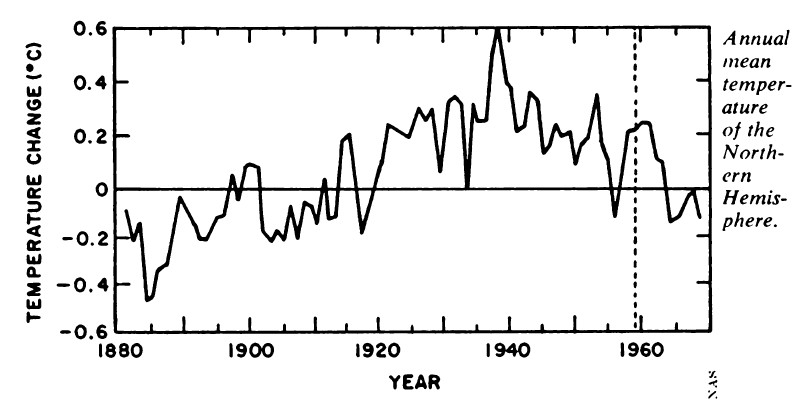
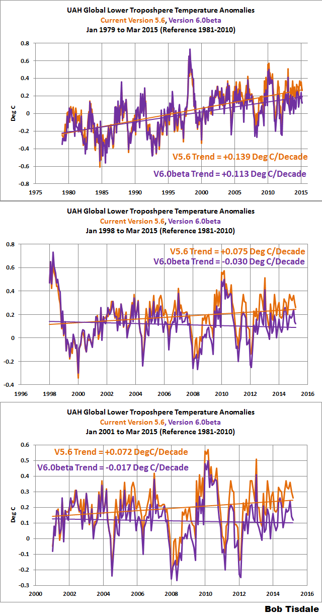
 .
.
Brandon Gates
May 13, 2015 at 12:19 am
David A wrote:
I am likely in support of fourth gen nuclear considering the safety factors, the 90 percent reduced waste with a vastly reduced 1/2 life, etc, but I do not get how coal in modern plants is so harmful?
Particulates: http://www.forbes.com/sites/jamesconca/2012/06/10/energys-deathprint-a-price-always-paid/
===============================================================================
Brandon, you missed the operative word. “Modern” coal plants. The particulates are well controlled and mitigated, unless you accept the poor and much disputed EPA reports. However the article you linked to was heavily invested into the massive particulate problem in India and China due to older coal plants, and in many cases to wood fires and dung for fuel as well.
“
David A says, “A straw-man for the skeptics position.” (regarding 500 million years ago CO2 levels disprove CAGW
Brandon says, “Not if your handle is MarkW or sturgishooper.”
=======================================================
I do not think one comment represents their entire position, and my comment referred to the skeptics position in general.
David A says, “
The 300 year to 800 year lag time of T rising first , before CO2 is supportive of the skeptical position, and works at time scales far more recent then 500 million years.”
Brandon says, ” My comments in (…) between his sentences.
” It does a bang-up job of confirming CO2’s solubility in water as a function of temperature, as known via too many lab experiments to count.” (Not cogent to my point or disputed, therefore another straw-man, and in no way does this support CAGW) Brandon continues, “Does not at all address CO2’s absorption/emission spectrum, nor does it refute Beer-Lambert law — both of which are undergraduate textbook material by dint of them also being the subject of once cutting-edge laboratory observation. (Not cogent to my point or disputed, therefore another straw-man, and in no way does this support CAGW)
Brandon continues Again, my comments in (…) between his sentences.
David A says, “Peer reviewed literature supports the three most recent warming periods in the last 10,000 years as being as warm or warmer then the current warm period The NH and global drop in T from the late 1940s to 1979 or so was a well established part of the record.” (Remember my point was that skeptic have no reliance on 500 million year old CO2 and T records)
Brandon responds, “Peer reviewed literature also supports the crazy notion that absorbed energy doesn’t just disappear into the aether, and is just as likely to be re-emitted in the general direction from whence it came as it is to be spat out in roughly the same direction it was going. Again, this is the stuff of basic physics texts.” (Not cogent to my point or disputed, therefore another straw-man, and in no way does this support CAGW or address my point)
Brandon continues
“Something else which is no surpise to the climate consensus community is that the so-called Holocene Climactic Optimum was indeed warmer than both the MWP and LIA. You know this because they know this. Yet you staunchly refuse to let their concern for present trends bother you, even though they’re the ones with the background and experience to give you the information you don’t dispute. Why?”
=======================================================================
Thanks for the question, but what a failed paragraph. First who is the climate consensus community?. Specifically who are the CAGW atmospheric specialists scientist, (note, not earth scientist or biologist who use the IPCC modeled mean to project future harms) who have publically stated that anthropogenic CO2 will result in disasters, and who has tallied their numbers against he skeptical scientist? Second, you skipped the Roman warm period, and I am grateful that even the ” the climate consensus community” accepts that the “so-called Holocene Climactic Optimum was indeed warmer than both the LIA” What you fail to note is peer review literature supports the MWP, the coolest of the three warm periods, as being as warm as today, and NO, the ” the climate consensus community” did not even exist when this was known so they did not inform me of this.
Brandon continues, ”
David A says, “The blip was likely removed for political, not scientific reasons.”
Brandon responds, “Silly me, I forgot that you’re a mind-reader and that when the scientific portion of your argument runs out of steam, imputing motive seamlessly takes over as if nobody will notice the switcheroo.
===============================================
Poor Brandon, You have never heard of political forces monetary gain, personal power, billion of dollars, peer pressure, or confirmation bias influencing human actions? I have directed you to books to read on the subject, so your dismissal of corruption in government is intellectually vacuous and willfully uninformed.
“David A continues, ”
If the AMO turns and the earth produces a decent La Nina, then all the warming since 1979 will likely vanish, and the Ice Age scare will commence again. This is called CGCYY. Catastrophic global climate yo yo.
Brandon says (My comments in (…..)
“What do you mean Ice Age scare will commence again? It never died on this blog. (This blog has nothing to do with the Ice Age scare, which really happened, “https://stevengoddard.wordpress.com/1970s-ice-age-scare/
and Mann recent poor paper on the slowing Atlantic current may be a prep for just such an event.) Brandon continues…
More substantively, a 4/10 degree drop is the most I could see …
… which puts us in 1990 territory, not 1979 …
… and since I trust these data and you don’t, I’ll take that bet in a heartbeat. As Simon alludes, the odd look pretty long against your favour” (Regarding Simon, like you he ignored cogent and relevant points of my post. I said a La Nina, in conjunction with a negative AMO, not just a La Nina. More specifically I am talking about the reverse of the very strong 1998 El Nino with the positive AMO. however, feeling generous, I will accept your .4 degrees of cooling, which puts us below 1979 temperatures.
I see about .3 degrees in the whole record, and sans the 1980’s el Chichon and 1990’s Mt. Pinatubo cooling, what have you got? CAGW? I think not. This would thoroughly decimate CS. to CO2, and likely elevate natural forces to their proper level.. AMO to NH temperature de-trended..
.
Chris Hanley says:
Brandon Gates’s commentary as in point 1) is based the premise that dangerous human-caused global warming requiring immediate radical mitigating action is occurring…
Brandon downplays that, but he stated very clearly not too long ago something just like it. He believes there is a serious problem occurring; that it is caused by human activity, and that major actions must be taken, in particular reducing CO2 to well below current levels.
I understand beliefs. We all have them. But science and the Western-originated scientific method are designed to put belief in its place. Skepticism of any belief is required for scientific progress. Otherwise, we are back to the witch doctor era. No one questioned the witch doctor. Scientific skeptics are essential to correcting misinformation. They do it by trying in every reasonable way to tear down any conjecture, hypothesis, or theory. That is the scientific skeptics’ job description. When they are successful, there is progress.
Skeptics point out that overwhelming evidence shows that the rise in CO2 has been a net benefit. There is no global harm identified due to the rise in CO2, which has been up to 20X higher in the past without ever triggering runaway global warming — the scare that started it all.
The rise in CO2 has also been clearly beneficial, measurably boosting agricultural productivity and thus keeping food costs down; a huge benefit to the ≈two billion people in the world who subsist on $2 a day or less.
If atmospheric CO2 was lowered to 350 ppm or less, there would be mass starvation. Is there any doubt? A plant growing in a pot doesn’t use soil to grow; as it gets bigger the soil level remains the same. Plant growth comes almost entirely from atmospheric CO2. More CO2 means more food, it’s that simple.
We didn’t plan to raise CO2 levels. That was a byproduct of fossil fuel use, another great benefit to humanity. But planned or not, the rise in CO2 has been entirely beneficial, and completely harmless. And it has clearly not resulted in the endlessly predicted global warming. That turned out to be almost completely wrong.
But still the alarmist crowd hangs their collective hats on demonizing CO2 (“carbon”). Take that away, and they’ve got nothing. Despite all the evidence to the contrary, they have decided to dig in their heels, and they adamantly refuse to admit that they were ever wrong about their CO2=cAGW conjecture.
They are willing to cause mass starvation of folks on the other side of the world, rather than acknowledge that their original premise has been proven to be completely wrong.
It’s hard to respect that.
David A,
That article was published June 10, 2012.
Table of figures from the article:
Energy Source Mortality Rate (deaths/trillionkWhr)
Coal – global average 170,000 (50% global electricity)
Coal – China 280,000 (75% China’s electricity)
Coal – U.S. 15,000 (44% U.S. electricity)
Oil 36,000 (36% of energy, 8% of electricity)
Natural Gas 4,000 (20% global electricity)
Biofuel/Biomass 24,000 (21% global energy)
Solar (rooftop) 440 (< 1% global electricity)
Wind 150 (~ 1% global electricity)
Hydro – global average 1,400 (15% global electricity)
Nuclear – global average 90 (17% global electricity w/Chern&Fukush)
Considering only estimated US coal mortality per unit energy and assuming US nuclear plants are NOT any less hazardous than the worldwide average:
15,000 / 90 = 167
According to the EIA [1], in 2014 the US generated 4.09 trillion kWh of electricity, 1.60 trillion kWh (39%) of that from coal. So:
1.60 * 15,000 = 23,944
If that energy had instead come from nuclear:
1.60 * 90 = 144
Which is better seen as annually accruing risk. So yeah, we’re far better off than China, but ~24 k premature deaths/year is nothing to sneeze at.
——————
[1] http://www.eia.gov/tools/faqs/faq.cfm?id=427&t=3
Serously?
The HCO is, by implicit definition, the warmest period of the Holocene. I didn’t “forget” anything.
Greed is a universal human traits. Corruption is one all too common manifestation of it.
How nice of you to once again assume you know what I actually think based upon things which I did not write. Ever hear of K Street? It’s not only environmental lobbyists who have set up shop there, you know.
My view is that he and I addressed them directly, and concluded by an appeal to data that returning to 1979 temperature levels, on the basis of internal variability alone, is unlikely. A sharp downturn in AMO in conjunction with sustained solar output decrease — plus throw in the odd major volcanic eruption on the order of Pinatubo, Krakatau or even Tambora — and sure … physically plausible and then some. Difficult to put odds on those sorts of events and even hairier to estimate the magnitude.
Why any of that should threaten the theory of radiative forcing due to CO2 is anyone’s guess — they are completely different physical mechanisms.
The internal variability estimates I provided are based on HADCRUT4, not UAH or RSS. From 1979 through 2014, the decadal rate of change for each is:
HADCRUT4 0.16
UAH TLT (v6 beta) 0.12
RSS TLT 0.12
0.12/0.16 * 0.4 = 0.3. Which is roughly 1990 levels for UAH and RSS, not 1979.
David A,
I missed some stuff first pass:
1) Beer-Lambert law is THE cogent point supporting AGW. CAGW is an open question.
2) The heck it isn’t disputed. Do you not read this blog? Have you not read THIS thread?
3) Solubility of CO2 in water as a function of temperature is the red herring. No serious climate researcher I am aware of disputes it. This is a non-argument.
Here’s MarkW: http://wattsupwiththat.com/2015/05/12/22-very-inconvenient-climate-truths/#comment-1932671
7) You really believe that a different configuration of the continents would be sufficient to completely compensate for CO2 being 20 times current levels? If that was true, then you have just admitted that CO2 is at best, a bit player in climate.
Here’s sturgishooper: http://wattsupwiththat.com/2015/05/12/22-very-inconvenient-climate-truths/#comment-1932768
Mean atmospheric CO2 content during the Cambrian Period: ~4500 ppm Mean surface temperature during the same: ~21 °C (~6 °C above present). Compute ECS.
Do you or do you not consider those two posters “skeptics”?
Oh, and here’s you from elsewhere: http://wattsupwiththat.com/2015/05/12/22-very-inconvenient-climate-truths/#comment-1933704
He apparently fails to realize that t CAGW is a single hypothesis, posed as a theory, and therefore skepticism of that is inclusive of every degree and manner of skepticism, competent or not.
Here’s you from just above: Remember my point was that skeptic have no reliance on 500 million year old CO2 and T records.
Feel free to make up your mind at any time.
Are you familiar with the saying, “The Devil may quote scripture when it suits his purposes”? Same principle, different epistemology. You accept, as do I:
Peer reviewed literature supports the three most recent warming periods in the last 10,000 years as being as warm or warmer then the current warm period The NH and global drop in T from the late 1940s to 1979 or so was a well established part of the record.
Yet you do not accept peer reviewed literature which says that continued warming is potentially hazardous.
Cue the next barrage of partisan claptrap pretending that liberal greenies are the only people on the planet playing politics with this issue.
Brandon Gates
You say in reply to MarkW
This is typical of your posts.
1.
You do not address the point made which is that nothing unusual is happening as there are precedents for all recent climate behaviours.
2.
You present a ‘straw man’; i.e. you make the untrue assertion of “continued warming” when the warming stopped nearly two decades ago.
3.
You present a fatuous assertion by claiming “continued warming” (which is not happening) “is potentially hazardous” but everything is “potentially hazardous” including getting out of bed in the morning.
4.
You apply an untrue assertion to the presenter of the point you have evaded; i.e. there is no evidence that “peer reviewed literature” (which you do not cite) has not been “accepted” by MarkW and any sensible person would accept that this “literature” is trivial if it only asserts that warming which is not happening is “potentially hazardous”.
Brandon Gates, you are a time wasting troll. All your posts fail to address the points made but introduce evasions, irrelevancies, ad homs ., and ‘straw men’ which would require pages of text to rebut.
Richard
At 1:30 AM on 14 May, richardscourtney responds to Mr. Gates‘ “Yet you do not accept peer reviewed literature which says that continued warming is potentially hazardous” with:
There is in such cases always a “cut to the chase” option that doesn’t oblige the respondent to treat with detailed rebuttal the sorts of dithering we keep getting from Brandon Gates. This route of consideration entails the inference of what we’ll call each respective warmist’s primary and secondary gain motivating his allegiance to this objectively insupportable (and factually unsupported) damnfool contention about the adverse effects of anthropogenic atmospheric carbon dioxide and – much more importantly – the political measures being pushed by each such statist sumbeech in order to allegedly ameliorate the tissue-of-lies “externalities” nonsensically asserted to be associated with the complete combustion of petrochemical fuels upon which all of industrial civilization depends for its function.
Mr. Gates‘ “science” is crap. We need not conduct a full lab analysis of his every bowel movement on this board (no matter how coprophically he presents it) in order to say that it’s crap. We’ve examined representative samples of his stool, and we’ve picked up the same pathological findings in each specimen, so it is appropriate parsimoniously to conclude that whether or not we get in there with a colonoscope and laboriously inspect every millimeter from the pectinate line to the ileocecal junction, we’re going to find nothing except Mr. Gates‘ peculiarly reeking dung.
He’s not doing this for reasons of interest in the “science.” He’s a political animal entirely, and his politics are poisonous.
What more need be said of him?
Oh, yeah. Not to mention the fact that there’s “peer reviewed” literature and then there are works which get into publication by way of broken-blinding “pal review.”
Mr. Gates goes with the flaming jackwad idiot premise that all peer review actions (indeed, all indexed publications) are equal in terms of validity, honesty – heck, infallibility.
Gotta wonder how much experience Mr. Gates has of the legitimate peer review process, either as an editor, reviewer, or author.
Betcha it’s friggin’ zip.
Brandon shrieked, “Temperature has risen since the beginning of the industrial revolution coinciding with a rise in CO2, and particularly since 1950 after which there was a marked increase in both the rate of emissions and CO2 accumulation in the atmosphere.”
Except when it has not::
http://woodfortrees.org/plot/hadcrut4gl/from:1937/to:1981/mean:12/plot/hadcrut4gl/from:1937/to:1981/trend
The above is over 40 years of cooling while CO2 concentrations accelerated.
And according to the NOAA:
“Near-zero and even negative trends are common for intervals of a decade or less in the simulations, due to the model’s internal climate variability. The simulations rule out (at the 95% level) zero trends for intervals of 15 yr or more, suggesting that an observed absence of warming of this duration is needed to create a discrepancy with the expected present-day warming rate.”
Over 40 years would be considered a rather large discrepancy.
The IPCC AR5 Technical Summary does not even mention the PDO, AMO or ENSO as being natural climate drivers during the industrial era. They state, “Solar and volcanic forcings are the two dominant natural contributors to global climate change during the Industrial Era.” I guess the IPCC did not get the memo regarding the PDO, AMO and ENSO.
Dear Skeptic, I once began a response to B.G as “Brandon bloviates” but his response became so personal (“reason had forsaken him, but he could still shout”) that I decided to regress from such strong attacks.
However I did mean it as a sincere criticism. If you read my two recent responses to him just above, along with my initial comments you will see his miss-direction tactics clearly. Brandon often conflates an irrelevant quote regarding some physics pertaining to the direct affects of CO2, having nothing to do with the point made or the evidence against CAGW. (Yet he sounds informed and the point is true, but in no way does it counter the argument presented.) He also likes to make complicated subjects appear to be simple minded conspiracies of the paranoid (like the well documented political motivations of politicians monetarily supporting the CAGW movement, and the corruption of the IPCC , also well documented, or the general corruption of peer pressure, confirmation bias, and noble cause corruption, all studied as very real by social scientists).
In doing the above he is competent in forcing a debating person to make long answers to poorly construed straw man arguments.
David A
I understand your frustration, but I write to provide a slight disagreement.
You rightly say of Brandon Gates
Your “above” implies that Brandon Gates posts information he understands. In fact, he often creates his straw men by copying&pasting to here long screeds which he does not understand.
It is his lack of understanding of what he posts that induces, for example, as you observe
He “sounds informed and the point is true” because he copies from other places that are “informed” but his copying “in no way does it counter the argument presented” because he lacks understanding of both “the argument presented” and what he copies.
He finds the stuff to copy by googleing so – although it is “irrelevant” – it has some relationship to the argument presented and, therefore, requires rebuttal.
In summation, Brandon Gates is a time wasting troll: he is not even a useful troll.
Richard
David A squealed, “Dear Skeptic, I ……” Just kidding.
Thanks for the comments and tip. I’ll try to tone it down.
Brandon stated, “The short rebuttal is that the 2nd law does not preclude a warmer body from absorbing energy from a cooler one. It only stipulates that net energy movement will always be in the direction of the warmer body to the cooler one. The word NET is the key here.”
I guess Clausius did not get your memo. The Second Law states:
“Heat can never pass from a colder to a warmer body without some other change, connected therewith, occurring at the same time”
The term “net” is nowhere to be found. That is your invention.
SkepticGoneWild,
Here’s the expanded quote: http://www.biodiversitylibrary.org/item/20044#page/100/mode/1up
This principle, upon which the whole of the following development rests, is as follows :–”Heat can never pass from a colder to a warmer body without some other change, connected therewith, occurring at the same time. Everything we know concerning the interchange of heat between two bodies of different temperatures confirms this, for heat everywhere manifests a tendency to equalize existing differences of temperature, and therefore to pass in a contrary direction, i. e. from warmer to colder bodies.
Emphasis added. How does a warm object “know” when to stop transferring heat to a cooler object?
It’s standard textbook thermodynamics. From the Wikipedia article on the 2nd law, immediately following the Clausius formulation:
The statement by Clausius uses the concept of ‘passage of heat’. As is usual in thermodynamic discussions, this means ‘net transfer of energy as heat’, and does not refer to contributory transfers one way and the other.
The Wikipedia article for black body radiation gives the following:
The net power radiated is the difference between the power emitted and the power absorbed:
http://upload.wikimedia.org/math/6/3/9/639daf0684603241b007dc69154c2253.png
Applying the Stefan–Boltzmann law,
http://upload.wikimedia.org/math/a/4/c/a4c6451a48ecec6d54b27fcf575c6500.png
“Brandon Gates : Most of these points have been rebutted a thousand times. Apparently at least 1,001 are required.”
ANSWER: thank you for your interest
“Truth n°1. The Mean Global Temperature has been stable since 1997, despite a continuous increase of the CO2 content of the air: how could one say that the increase of the CO2 content of the air is the cause of the increase of the temperature?
“a) Temperature has risen since the beginning of the industrial revolution coinciding with a rise in CO2, and particularly since 1950 after which there was a marked increase in both the rate of emissions and CO2 accumulation in the atmosphere.”
ANSWER: This assumed covariation has been demonstrated incompatible with the data series of T(t) an [CO2](t) ; the only possible correlation is between d[CO2](t)/dt and T(t) according to statistical tests well known in econometrics; since 1950 , the temperatures have been declining up to 1975, then going up 1975-1996 and are about stable since; lower troposphere global coverage by satellite remote sensing by microwave sensors began end 1978, and those series are to be preferred due to the problems of the terrestrial meteo stations discussed on WUWT. See figures 20-A, 20-B,
“b) Time evolution of radiative forcing from CO2 has been observed directly from both satellite- and ground-based instruments in the spectral bands predicted by line-by-line radiative models fed data from laboratory analysis of CO2.”
ANSWER: I should be happy to learn on those measurements at the tropopause !
The global OLR has been more or less stable since 1974 (figure 21-C) and did not show the regular decrease expected according to Myrhe’s formula while the ppm went from 333 ppm in 1974 to 400 ppm. The oceanic calorimeter may have see the ocean heat content increase by some 140 to 180 ZettaJoule since 1960 but the cumulative radiative forcing is about 1200 to 1500 ZettaJoule, seven times more ! Where did the remaining 1000 to 1300 ZettaJoule go ? IPCC AR5 WG1 page 67 (TFE.4 figure 1) is well aware of the “problem” but assumes an increase of the OLR by about 3 W/m² over the time span 1970-2010: that is not seen in the global OLR series of observations (figure 21-C).
“c) Internal variability is still dominant over short-term (annual/decadal) timeframes”.
ANSWER: Internal variability or “cycles” are well documented: see figures 5-B and 5-C for the 1000 year “cycle”, many papers for the 210 year de Vries cycle (prominent in 14C and 10Be observations of the solar magnetism); for the “60 years” see Truth n°5. If all observations can be explained by such “cycles” there is no need to invoke supra-natural “radiative forcing” by trace gases. The cooling of the stratosphere (lower strato) following each of the volcanic dusts episodes may be related to the automatic cooling of the lower stratosphere when the temperature of the surface increases: this obvious mechanical compensation is described and explained in the old V. A. Belinskii Dynamic Meteorology Ogiz Moscow 1948, The Israël program for scientific translations 1961, 592 pages. Those coolings (after Agung, El Chichon and Pinatubo, but no cooling since 1995) explain the small decrease of the CO2 OLR radiating from layers above the tropopause near 220 K to 230 K.
“Truth n°2. “37% of the cumulative anthropic emissions since the beginning of the Industrial revolution have been emitted since 1997, …” ” See point (c) above. Add: it’s no mystery to climate literature that sometimes internal variability …”
From Vostok and other ice cores we know that it’s the increase of the temperature that drives the subsequent increase of the CO2 content of the air, thanks to ocean out-gassing, and not the opposite. The same process is still at work nowadays] (discussion: p. 7)
“Yes, the outgassing process is still operative today because the laws of physics did not suddenly decide to change. ”
ANSWER: Yes indeed !
“amplify the temperature response to external forcings …”
ANSWER: For a completely carbon-dioxide-free reconstruction of the Vostok temperatures since 450 000 years refer to O. G. Sorokhtin (references on card n°7) chapter 4.4 pp. 180-190 Precession Cycles and the Earth Climate: it explains in detail and computes the quick de-glaciations observed by G.Roe and by Lisiecki & Raymo, with all the “saw-teeth”.
“The sawtooth wave form is particularly consistent with the so-called “greenhouse” effect due to thermal radiative gasses which reduce the rate of heat loss”.
ANSWER: Those tales of “blankets” are super-natural or anti-physical: the cooling of the surface is mostly by evaporation or evapotranspiration; as the net radiative heat transfer surface to air is about nil as explained at length in truth n°6.
“3. The amount of CO2 …no more than 6% of the total CO2 in the air ….the non-anthropic (or natural) delta13C becomes very slowly more negative … which is THE signature of burning fossilized plant matter… ”
ANSWER: No ! There are 24 ppm at -29 pm (anthropic fossil fuel and gas) and 376 ppm at -7 pm (natural); the first is purely anthropic and the 376 ppm (natural) have a decreasing trend as the organic remains oxidized today have the delta13C signatures of the time they were living; remineralisation in the soil takes weeks to centuries depending on the size of the bacteria or of the trees ….
“… with the replacement of CO2 molecules absorbed by the vegetation by molecules out-gassed from soils by the oxidation of the organic material of plants grown years to centuries before: the delta13C of the air was then slightly less negative. … Which argument is given without a whit of substantiation and not a proposed causal mechanism in sight.”
ANSWER: as said the delta13C of the rotting remains is that of the time when the plant or the animal was alive.
“4. The lifetime of CO2 molecules in the atmosphere is about 5 years instead of the 100 years said by IPCC. (discussion: p. 10) ……………………. This conflates the average lifetime of a single molecule with the decay of atmospheric concentration following an increase above equilibrium levels. The notes on this point are self-contradictory: This derivation of [CO2](t) does not assume any given equilibrium between ingress and egress …”
ANSWER: the only assumption made is that absorption is proportional to the CO2 content of the air; it applies equally to the both parts or sets of molecules of the air, the anthropic (24 ppm) and the natural (376 ppm); this makes NO hypothesis about ingress”
“… followed almost immediately by: foutgassing(t) – fabsorbed(t) = k (T(t)- T0) … which is an equilibrium formulation.
ANSWER: : this is not an assumption but an observation see figure 17-B; it applies to the natural set of molecules; I would not call it “equilibrium” as it is temperature and time and latitude dependent; the natural outgassing and the absorption of “natural” molecules occur in quite different places (ocean) or at different seasons or times (land).
“5. The changes of the Mean Global Temperature are more or less sinusoidal with a well defined 60 year period. …. True, but fails to explain why the longer-term mean about which those cycles fluctuate is trending up other than curve-fitting an “approximation by three sinusoids of periods 1000 years, 210 years and 60 years,”
ANSWER: The curve fitting exercise is labeled as such “heuristic”; the lengths of the cycles are from other observations, some displayed on figures 5-B & C ; only the amplitudes and phase of the 215 and 60 years sinusoids are subject to optimization; Singular Spectrum Analysis has been applied by Diego Macias et al (note 18) to the HadCRUT series with equivalent results, and among many others by Liu Yu et al. Amplitudes, rates, periodicities and causes of temperature variations in the past 2485 years and future trends over the central-eastern Tibetan Plateau Chinese Science Bulletin Oct. 2001 with a forecast- temperature decrease 2006-2060…
The “trending up” is a consequence of the phase of the longer “1000 years” and “210 years” cycles, with n assumed maximum over 2000-2020.
” 6. The absorption of the radiation from the surface by the CO2 of the air is nearly saturated. … Oh dear. Radiation extinction over a given path-length is not “CO2 saturation”. Extinction is, however, the primary mechanism by which the so-called “greenhouse effect” operates.”
ANSWER: by “saturation” is usually meant a complete absorption of the radiation of the surface by the carbon dioxide and water vapor of the air: according to Dufresne and Treiner it is saturated and according to Pierrehumbert (Physics Today 2011) it is not; for me 0.8 (W/m²)/400 = 0.2% for a doubling of the CO2 content is” nearly saturated”; 0.8W/m² is the additional absorption for 2xCO2 (e.g. per Hansen 1981)
“8. The sea less than 1.3 mm/year. (discussion: p. 18) ..And yet landed ice mass loss is accelerating. Where is the water going? Not into the atmosphere according to this article.”
ANSWER: to complement the card : the psmsl.org data base has some very interesting measurements of the changes of pressure on the bottom of the ocean with no obvious trend since 1993 (South Drake passage)… where is the +3 mm/year gone ?
“9. The “hot spot” in ..The tropical tropospheric hot spot prediction is not based on water vapour feedback to warming, and it is especially not unique to warming due to any other GHG forcing. In short, it is not a “fingerprint” of AGW. ….The primary mechanism is increased atmospheric convection from the surface. Observations of the tropical troposphere are not in good agreement with each other, so declaring this a fatal modelling flaw is not a tenable argument. Calling it a problem for CO2 radiative forcing is bizarrely wrong.”
ANSWER:
(1) PNAS , oct. 22, 2013 Ben Santer et al name it a fingerprint of the anthropic influence (ANT)
(1 bis) Santer, B.D et al. Consistency of modelled and observed temperature trends in the tropical troposphere. Int. J. Climatol. 2008, doi:1002/joc.1756
(2) for the IPCC AR4 report : http://www.ipcc.ch/publications_and_data/ar4/wg1/en/figure-9-1.html
see comments http://www.drroyspencer.com/2009/10/hotspots-and-fingerprints/ : ” it is this “warming and humidifying of the global atmosphere” and the resulting “acceleration of the hydrologic cycle” that creates the upper troposphere hotspot. Ergo, no hotspot means no powerful water vapor amplification mechanism and no CO2-based account of late 20th century warming
(3) for the IPCC TAR see http://climateaudit.org/2008/12/28/gavin-and-the-big-red-dog/
(4) the hot spot has been discussed in IPCC AR2 as a proof of the human causation see references and discussions in http://www.americanthinker.com/articles/2013/11/ipcc_s_bogus_evidence_for_global_warming.html
“10. The water vapour content of the air …. Water vapour content is largely a function of temperature, particularly ocean surface and near-surface temperature. The oceans are frigid at depth, and the rate at which those cool waters are exposed to the surface is not constant. The balance of the note goes on to ignore:… by throwing up lots of plots showing wv content in the upper layers of the atmosphere”.
ANSWER: the role of the upper layers of the water vapour (wv) on the OLR has been said on figures 6-C and 6-D ; less wv means a higher OLR over significant parts of the water vapour spectrum (figure 6-A) compared to the ten(s) of cm-1 of the tropospheric CO2. The “lower and warmer” wv mechanism compensate the “higher and cooler” effect said for CO2 near 600 cm-1 and 720 cm-1.
This effect at 200 mbar to 400 mbar is unrelated to the “frigid depths of the ocean”
“13. The measurements .. Mention of significant regional difference may suggest more abject cherry-picking …”
ANSWER / QUESTION: does this insult refer to the observations of Argo buoys collated by the Scripps Institution (figure 13 A) ?!
“15. The Stefan Boltzmann …remembers that ε is not constant for all materials at any given wavelength”
ANSWER: it is k(nu, P, T) that is wavelength dependent not epsilonn ; the annex 15-A shows an example of abuse of the SB formula
“16. The trace gases ….. The short rebuttal is that the 2nd law does not preclude a warmer body from absorbing energy from a cooler one. It only stipulates that net energy movement will always be in the direction of the warmer body to the cooler one. The word NET is the key here.”
ANSWER: it has been said again and again that (truth n°1 and elsewhere): The radiative heat flow from a body A to a body B is: (radiation from A absorbed by B) minus (radiation of B absorbed by A) … what you call “net”
“17. The temperatures have …. This is basically a repeat of previous points about Vostok ice cores”.
ANSWER: The most important point is figure 17-B, a direct proof from observations that d[CO2]natural /dt = k (T(t)- T0)
“18. The CLOUD And the fatal problem for AGW is … what?”
ANSWER: Since 1998 (http://journals.aps.org/prl/abstract/10.1103/PhysRevLett.81.5027) and 2007 (Svensmark & Calder The Chilling Stars: A New Theory of Climate Change) the findings of the danish group have been corroborated by a group of specialist of the planetary magnetism in Paris and Moscow with two distinguished members of the French Academy of sciences, since 2005: Jean-Louis Le Mouel, Kossobokov, Courtillot et al. On long-term variations of simple geomagnetic indices and slow changes in magnetospheric currents: The emergence of anthropogenic global warming after 1990? Earth & Planetary Science Letters (2005) and many papers afterwards
If the solar magnetism is very closely correlated to temperatures, then there is no need of carbon dioxide and “forcing” based tales to explain the observations.
“19. Numerical “Climate models” … This is a climate modelling issue, not a fundamental challenge to GHG radiative forcing. An aside: one of the reasons that clouds modulate temperature so effectively is not just the albedo increase which bounces downwelling short wave radiation back into space, but because they radiate IR back to the surface thus reducing the net rate of thermal radiative loss.”
ANSWER: several of the “truths” have shown that the “GHG radiative forcing” is NOT a physical effect but, from its very definition by IPCC, a computational trick that assumes that the tropospheric temperature and humidity are kept constant … during up to 200 years (the time needed to double the ppm of CO2 at +2 ppm/year).
In addition as explained on page 5 (truth n°1) GH= (radiation from the surface) minus (outgoing longwave radiation (OLR) has NO physical meaning as energy and cannot be added as done ( for instance Lacis, Hansen et al. Tellus 2013) to the real solar energy absorbed by the surface.
To be energy or more properly, heat transferred, the one-way upwelling radiation from the surface absorbed by the air should be reduced by subtraction of the down-welling radiation of the air absorbed by the surface
Note that by subtraction of the (about 20 W/m² in global average) flow surface to cosmos of both terms of GH, GH expression becomes
GH= (radiation from the surface absorbed by the air ) minus (outgoing longwave radiation from the air)
which has absolutely no physical sense !
To get a physically valid quantity you have to add the radiation of the cosmos absorbed by the air (a few µW/m²) and to subtract the radiation of the air absorbed by the surface.
“20. The forecasts … A forward-looking AOGCM is not used to “prove” CO2-driven AGW. Evidence of that comes mainly from past observation.”
ANSWER: Observations are the time series T(t), [CO2](t) and emissions(t); as d[CO2]natural(t)/dt correlates with T(t) and as no other correlation is (mathematically) allowed (by statistical tests) then the [CO2 natural] is, as shown as well on figure 17-B, a consequence of the past temperatures (their time integral) and cannot be their cause.
This proves that there is no and can be no evidence of “CO2-driven AGW”
Camille,
No. The Myhre relationship T = α(C/C₀), which is a time-independent expression of equilibrium climate sensitivity, can be used to estimate transient response to CO2 forcing for an arbitrarily short period of time, with the caveat that arbitrarily short does not mean a week, a year, or even a decade. Half a century works well for me, but I get the best results using 1850 or 1880 to present.
At TOA is most common and robust. At the surface is next, and getting better as more ground-based stations directly measuring downwelling radiation across the spectrum by wavelength are deployed.
AS in my original post, OLR is a function of temperature according to the Stefan-Boltzmann relationship, not Myhre: j = σεT⁴
When measured from space, OLR is going to pick up two things:
1) LWR direct from the surface and cloud tops in the so-called “atmospheric window” spectral bands.
2) Re-emitted LWR from GHG molecules at altitude.
Particularly since cloud cover varies, OLR as seen from space does not make for a good indicator of surface temperature. This is why RSS and UAH use the microwave band for taking atmospheric temps, not infrared sounders, and why we still used ground-based thermometers for the surface.
A relevant quote from that section:
As the climate system warms, energy is lost to space through increased outgoing radiation. This radiative response by the system is due predominantly to increased thermal radiation, but it is modified by climate feedbacks such as changes in water vapour, clouds and surface albedo, which affect both outgoing longwave and reflected shortwave radiation. The top of the atmosphere fluxes have been measured by the Earth Radiation Budget Experiment (ERBE) satellites from 1985 to 1999 and the Cloud and the Earth’s Radiant Energy System (CERES) satellites from March 2000 to the present. The top of the atmosphere radiative flux measurements are highly precise, allowing identification of changes in the Earth’s net energy budget from year to year within the ERBE and CERES missions, but the absolute calibration of the instruments is not sufficiently accurate to allow determination of the absolute top of the atmosphere energy flux or to provide continuity across missions.
Since it’s not been observed going out — which is where your note about OLR does become relevant — it must have stayed in. Note here the difference between precision and accuracy. When counting joules in absolute terms you need accuracy, which ERBE and CERES do not have. For net flux calculations to derive energy balance, precision is the main requirement, which ERBE and CERES provide.
I don’t like it that Trenberth can’t account for the missing heat any more than he does, but 1st Law triumphs over energy-destroying hobgoblins every time.
Big if. Here’s the point where I issue my standard challenge: build an AOGCM which explains the past 2,000 years to present better than CMIP5 without invoking any atmospheric radiative transfers from CO2 and you’ll have my full and undivided attention. Until then, you’re just making noise.
I think I agree with you there. What I don’t understand how that in any way challenges CO2’s radiative role in the lower troposphere.
How about a quick summary instead.
You must be a fan of electric blankets then.
Academic. You know this because every working climatologist today knows this.
lol. No. n°6 gave me a headache the first time I read it. The main thesis is The absorption of the radiation from the surface by the CO2 of the air is nearly saturated and then goes on to talk about everything but. We have direct observation from ground-based instruments which measure downwelling and upwelling LWR separately and the results are entirely consistent with Trenberth’s energy budget cartoon, from whence it is we also find the surface fluxes for convection and evapotranspiration.
Try this: http://www.esrl.noaa.gov/gmd/grad/surfrad/
I’ve spent countless enjoyable and self-educational hours crunching data downloaded from their servers.
Absent our influence, or major environmental disruptions, the carbon cycle is based on equilibrium processes …
… and you are proposing that something other than us has disrupted that equilibrium process. So, if not us, what?
I’m not quibbling about whether it’s an assumption or an observation. It’s an equilibrium formulation plain and simple. Understand and own it as such no matter how it is derived.
Such correlations want a plausible physical mechanism associated with them to be compelling. The radiative forcing of CO2 has such a plausible physical mechanism, as does the observed fact that absorbed solar energy tends to warm things up. The nifty thing is that CO2’s radiative properties explain the predicted and observed stratospheric cooling to boot.
Venus also makes a lot more sense when one takes the time to learn about the actual first principles of physics from readily available standard texts on the subject.
No. I wrote earlier that “complete absorption” is another way of saying “extinction” which is not precisely correct because extinction can occur without absorption — refractive and reflective scattering will do it as well. Complete absorption is THE reason that potent GHGs like water vapour and CO2 reduce the rate of heat loss from the surface and lower levels of the atmosphere. Look up Beer-Lambert law for the beginning of the explanation.
What is generally meant by “the CO2 effect is saturated” is that additional concentrations of the gas will not have any additional radiative effect. Explanations vary, and every one I have ever read has been utter nonsense. Increasing the optical thickness of a medium at any wavelength only ever increases its ability to ultimately scatter a beam of radiation at that wavelength attempting to traverse it.
I have no clue. How about you tell me.
No: We perform a multimodel detection and attribution study with climate model simulation output and satellite-based measurements of tropospheric and stratospheric temperature change. We use simulation output from 20 climate models participating in phase 5 of the Coupled Model Intercomparison Project. This multimodel archive provides estimates of the signal pattern in response to combined anthropogenic and natural external forcing (the fingerprint) and the noise of internally generated variability. Using these estimates, we calculate signal-to-noise (S/N) ratios to quantify the strength of the fingerprint in the observations relative to fingerprint strength in natural climate noise.
The “fingerprint” they’re looking for here is both natural and anthropogenic external forcings as opposed to internal variability in BOTH the troposphere and stratosphere.
Abstract does NOT call tropical stratospheric warming THE fingerprint. Here it is in full:
Abstract
A recent report of the U.S. Climate Change Science Program (CCSP) identified a ‘potentially serious inconsistency’ between modelled and observed trends in tropical lapse rates (Karl et al., 2006). Early versions of satellite and radiosonde datasets suggested that the tropical surface had warmed more than the troposphere, while climate models consistently showed tropospheric amplification of surface warming in response to human-caused increases in well-mixed greenhouse gases (GHGs). We revisit such comparisons here using new observational estimates of surface and tropospheric temperature changes. We find that there is no longer a serious discrepancy between modelled and observed trends in tropical lapse rates.
This emerging reconciliation of models and observations has two primary explanations. First, because of changes in the treatment of buoy and satellite information, new surface temperature datasets yield slightly reduced tropical warming relative to earlier versions. Second, recently developed satellite and radiosonde datasets show larger warming of the tropical lower troposphere. In the case of a new satellite dataset from Remote Sensing Systems (RSS), enhanced warming is due to an improved procedure of adjusting for inter-satellite biases. When the RSS-derived tropospheric temperature trend is compared with four different observed estimates of surface temperature change, the surface warming is invariably amplified in the tropical troposphere, consistent with model results. Even if we use data from a second satellite dataset with smaller tropospheric warming than in RSS, observed tropical lapse rate trends are not significantly different from those in all other model simulations.
Our results contradict a recent claim that all simulated temperature trends in the tropical troposphere and in tropical lapse rates are inconsistent with observations. This claim was based on use of older radiosonde and satellite datasets, and on two methodological errors: the neglect of observational trend uncertainties introduced by interannual climate variability, and application of an inappropriate statistical ‘consistency test’.
Which is pretty much exactly what I wrote in my original response with a few additional details about reconciling the differences between observational datasets.
Here’s the caption: Figure 9.1. Zonal mean atmospheric temperature change from 1890 to 1999 (°C per century) as simulated by the PCM model from (a) solar forcing, (b) volcanoes, (c) well-mixed greenhouse gases, (d) tropospheric and stratospheric ozone changes, (e) direct sulphate aerosol forcing and (f) the sum of all forcings. Plot is from 1,000 hPa to 10 hPa (shown on left scale) and from 0 km to 30 km (shown on right). See Appendix 9.C for additional information. Based on Santer et al. (2003a).
Note in panel (a) solar forcing that, aside from the high northern latitudes, the most warming also occurs in the tropics between 200-300 hPa, but that unlike in panel (c) well-mixed greenhouse gasses that the warming goes all the way to TOA. The marked cooling beginning at about 75 hPa and going to TOA in the GHG panel are THE anthropogenic fingerprint in this graphic.
As I mentioned previously, any increased external forcing is expected to produce a tropical tropospheric “hot spot” by way of deep convective processes in the equatorial oceans — it is not at all specific to GHG — or CO2 — forcing whatsoever.
But when cooler water from depth is manifest at the surface, which it does in cycles, it IS relevant to wv content at 1000 mbar. Plotting wv content against CO2 concentration is ridiculous to the extreme — CO2 does not regulate wv content. SST however, does.
I wrote: Figure 13-B Ocean Heat content of the North-Atlantic (30°N-65°N) from 1955 to 1st Q 2014.
What do you think?
http://www.deltat.com/pdf/Infrared%20Energy,%20Emissivity,%20Reflection%20%26%20Transmission.pdf
Non-Greybody Materials
A non-greybody material is one that has a different emissivity value at different wavelengths. For opaque materials the tendency for the emissivity to vary with wavelength is typically due to the physical size of the microscopic surface features of the material. For non-greybody materials, the tendency of the material to absorb, reflect or transmit infrared energy varies with wavelength. Non-opaque non-greybody materials called selective emitters are discussed in a separate section below.
So when is it going to dawn on you that rate of heat flow from warm to cool is dependent upon how far away from zero net flux is?
That section ends with:
constant increase of the [CO2] content of the air = temperatures stable w.r.t to the reference T0
Conclusion: The CO2 content of the air is a consequence of the temperature(s) and can not be their cause
The former statement is not in dispute. Solubility of CO2 in aqueous solution as a function of temperature is basic 1st year chemistry. The latter statement is purest rubbish of the most woefully ignorant possible. For the love of all that is rationally logical, what does CO2’s tendency to come out of solution as T goes up have to do with the radiative properties of the molecule in its gaseous phase in the atmosphere?!
If the solar magnetism is very closely correlated to temperatures, then there is no need of carbon dioxide and “forcing” based tales to explain the observations.
Here’s the abstract:
Abstract
During the last solar cycle Earth’s cloud cover underwent a modulation more closely in phase with the galactic cosmic ray flux than with other solar activity parameters. Further it is found that Earth’s temperature follows more closely decade variations in galactic cosmic ray flux and solar cycle length, than other solar activity parameters. The main conclusion is that the average state of the heliosphere affects Earth’s climate.
Nothing in there precludes a radiative role for CO2, water vapour or any other IR-active species. If you think it does, then you also need to believe that this paper “proves” that TSI is an irrelevant solar activity parameter.
Is that a “mu” before W/m²? As in micro Watts per square-meter? Really?
I’m completely out of original ways to respond to these rubbish false dichotomies, except to wonder out loud where it is written in statistical texts that there is only one allowable mathematical model for a T to CO2 relationship.
Brandon,
constant increase of the [CO2] content of the air = temperatures stable w.r.t to the reference T0
Is worse than you thought: Henry’s law is:
ΔpCO2 = k*(T-T0)
where k = ~8 ppmv/K (4-17 ppmv/K according to the literature).
Point 17 in the article says:
dCO2/dt = k*(T-T0)
which means whatever small change in temperature you have, CO2 will rise in the atmosphere until eternity, without any feedback from the increased pressure of CO2 in the atmosphere. That is pure nonsense and only based on curve fitting of two straight lines (T increase and dCO2/dt increase) thereby attributing T for the full rise in dCO2/dt. That is based on the excellent fit of the variability of T and dCO2/dt, but variability and trend have nothing to do with each other: variability is caused by the temperature influence on (tropical) vegetation, while the trend is not caused by vegetation changes (vegetation is an increasing sink for CO2)…
In reality, the slightly quadratic increase of human emissions over time are twice the increase in the atmosphere and are the main cause of the increase.
The real formula for the rise of CO2 with temperature is:
dCO2/dt = k*(T-T0) – ΔpCO2
where ΔpCO2 is the rise in CO2 since t= 0. as ΔpCO2 increases over time, dCO2/dt goes to zero. At that moment we get:
ΔpCO2 = k*(T-T0)
which is what Henry’s law says…
Ferdinand Engelbeen,
Yes that is worse than I thought, good catch.
Which is sane and really shouldn’t be at all controversial.
Point 16 and the associated commentary encapsulate the kind of fallacy that makes it all-too easy for mainstream scientists to dismiss all ‘skeptics’ as cranks. The author misrepresents the 2nd law of thermodynamics and then compounds the felony by propounding a doctrine (the idea that gravity by itself can create a permanent gradient of temperature in an atmosphere) which really does violate the law. One can imagine that gravity could in special circumstances produce a temporary gradient of temperature, e.g. if a planet previously without an atmosphere acquires one by passing through a cloud of gas, but what is then to maintain the gradient against the tendency for heat to be equalised throughout the atmosphere? Or simply radiated into space?
I agree David, most of the points made are very credible but point 16 is simply wrong. The true situation is that without the green house gas the surface radiates to space which is at 4K while with ghg it radiates to to ghg at a temperature around 200K or higher. The back radiation from a 4K source is far less than from a 200K source so the net energy loss (radiated energy – received energy) is greater when radiating to space so the surface temperature will be lower. Just as you feel colder standing outside on a cold winters night compared to standing in a warm room.
His point 6 is also wrong. Yes at the line center the absorption of CO2 is “saturated: – surface emission totally replaced by emission from the top of the ghg column but as the conc of the ghg increases, the line width increases so the ghg starts to absorb over a greater and greater range of wavelengths – this is the cause of the logarithmic relationship between concentration and absorption.
I did not read that “the idea that gravity by itself can create a permanent gradient of temperature in an atmosphere” other then the idea that atmospheric density by itself creates greater heat capacity, thus a longer residence time for energy to saturate while insolation continues unabated. This is not controversial.
Replying to David A (comment of May 12 at 10:41 p.m.)
The author says ‘There is no need of heat to “warm the surface” because its temperature is a consequence of the gravitation and of the mass of the air, both on Earth and on Venus.’
I’m not sure what he means by this, but I took him to be endorsing the ‘theory’ that gravity by itself is responsible for a temperature gradient in the atmosphere. This seems to be quite a popular idea in some quarters. The phrase ‘there is no need of heat to “warm the surface”‘ does seem to imply a source of heat other than solar radiation, and the author immediately goes on to mention gravitation. Indeed, for anyone who denies the basic principle of the greenhouse effect, as the author seems to, there is a need to explain why the average temperature at the surface of the Earth (or Venus) is higher than it ‘should’ be at the relevant distance from the Sun. Hence the appeal to gravity! But as I pointed out in my comment, any gravitational heating effect due to compression of the gases in the atmosphere would only be temporary, as the heat would be dissipated by radiation.
But if you don’t think this is what the author meant, feel free to ignore my comments.
To Richard C; thanks, and essentially I agree with “Your “above” implies that Brandon Gates posts information he understands” in that I am often not certain he even understand the simple CAGW criticism made, as he often does not respond to that message. However I will stipulate that my comment was meant to imply that Brandon’s competence, was in the direction of forcing long answers to simple statements he makes, like calling anyone that implies that billions of political dollars and the politics of government power have a corrupting influence on the science, a “paranoid conspiracy nut” So, in a sense, I was politely calling him a competent troll.
I wavier in this, in that sometimes he is good at refuting poor skeptical arguments, although he usually includes the a gratuitous insult at the entire skeptic community in that response. He apparently fails to realize that t CAGW is a single hypothesis, posed as a theory, and therefore skepticism of that is inclusive of every degree and manner of skepticism, competent or not. Sometimes he clearly grasps what he is talking about, at other times he is simply arm waving like a hummingbird and even if he perfectly understands his own post, it is not cogent to the skeptical argument conveyed, nor does the technical correctness of it, in any way support CAGW.
I take the time to go point by point through his posts, because the may confuse a person new to the subject of CAGW. I always appreciate your posts Richard. Much thanks
David A
David quotes, “‘There is no need of heat to “warm the surface” because its temperature is a consequence of the gravitation and of the mass of the air, both on Earth and on Venus.’
=========================================================================
The first part is a bit ambiguous, but the second in no way attempts to refute down welling radiation. The density of gas molecules, caused by gravity, is the primary element determining their heat capacity. Take the same single gas in an atmosphere. Heat them all to the same. The amount of the gas, in conjunction with the gravitational pull of the planet, determines how hot each sq meter is. Raise a thermometer through the atmosphere of the same molecules vibrating or moving at the same T. As the thermometer rises, it will record an ever lower T as fewer molecules strike the thermometer. This is due to gravity.
David A,
I don’t think I’ve used those exact words on this blog, as that’s one of the the surest way to the bit bins there is. Elsewhere I’ve said far worse, but not because I’ve drunk the Kool-Aid that graft and corruption absolutely do not exist at all levels of gummint when there are monies from the public till to be had by any vested interest.
Difference between you and me so far as I can tell is that my method for looking out for it is to evaluate the actual claims being made and seeing if I can reconcile them against first principles used across multiple disciplines. For AGW, that is rather easy, as the basic physics have been on the books since the 19th century, and because I first learned of them in high school textbooks.
Such a gentleman.
I reserve my most scathing individual jibes for those who misrepresent my words.
You apparently fail to recognize, repeatedly, that you’re a lousy mind-reader. I’m quite well aware that there is no one school of climate contrarianism, which fact can be a source of frustration. Selective data acceptance is one of my most persistent annoyances, though it can be darkly amusing — and quite telling — to be accused of denying a particular data point when in fact what I dispute is the interpretation of it.
I do agree with you that there is one single hypothesis about the main cause of AGW. There is NOT one single hypothesis about the putative effects. Your first clue should be the published range for ECS: 1.5-4.5 K per doubling of CO2. It was a valiant effort on your part to attempt to fit we “alarmists” into one box, but sorry, no dice. I assure you, we warmies are no more monolithic in our understanding of the relevant science, nor our views on what the risks are, and especially not the solutions we prefer and certainly not how we think best to go about implementing them.
Funny how it’s ok for you to use the broad brush, but not me, isn’t it. This aggravates me almost as much as selective data acceptance. Ooh, and vastly unequal standards of proof. That last one really turns my crank.
reply for David 7:14 am and David A
from dP= -rho g dz (barometric equation), rho = P/(RT) and dH= Cp dT – dP /rho and dH= Ch dT you get the well known relation between pressure and temperature ; one partial case is the adiabatic Ch=0; the tropospheric temperature gradient g/(Cp+ Ch) is a function of the gravitational acceleration 9,8 m/s²
The use of the word “heating” or “gravitational heating” or “additional heat” is quite misleading because there is no “heating”; the temperature is related to the pressure! Ascending air cools
The only heating is from solar infrared (absorbed by water vapour) and condensation (of water vapour); the heating in the altitude explains the Ch.
This heating of the air “from above” explains the fact that the lapse rate is between-5 K/km to – 8 K/km depending on the exact value of Ch at the place , altitude and time considered and not the adiabatic lapse rate of -9.8 K/km.
The changes of the temperatures with compression and expansion are well explained in many text books and in practical equipment since the machines of James Watt (about 1750-1780)
The radiative cooling occurs only on the top layers (around the surface of optical thickness t=1 from the top of the air as shown on figure 6-C and 6-D; it is compensated by the heat delivered by absorption of solar infrared and by condensation.
There is no radiative effect or radiative transfer of heat across an opaque material like the air (figure 6-A except in the window where 20 W/m² go un-intercepted from surface to cosmos).
As explained at length in the post the only radaitive effect is the cooling of the “top of the air” at the optical frequency of interest (localized as pressure versus optical frequency in figures 6D or 6-C)
“12. The sum of the surfaces of the Arctic and Antarctic icepacks is about constant, their trends are phase-opposite; hence their total albedo is about constant. (discussion: p. 25)”
Actually, this means that earth’s albedo is increasing, since Antarctic sea iceis about five times as reflective as Arctic, due to its stretching farther toward the equator, being lighter in color and other physical reasons.
I’m not sure how the sum of their surfaces could possibly be seen as constant when they’re both busy losing massive amounts of ice. ps – The gains in Antarctic sea-ice are miniscule by comparison to losses in land ice.
Douglas Hollis
?? We’ve stated before that the simple “sum” of Arctic sea ice and Antarctic sea is misleading – The Antarctic sea is much more important over the course of the year than the Arctic, at times receiving 5 times the energy that the Arctic sea ice gets. 8 months of the year, the slowly decreasing Arctic sea ice actually allows more heat to be lost from the Arctic ocean that it gains from the very low sunlight levels that are present due to increased evaporation, convection, conduction and radiation losses.
You are wrong about Antarctic land ice … the actual losses are conjecture only “measured” after assumed geological rebound numbers are inserted into the GRACE data. The gains in Antarctic sea ice – the sea ice area that DOES MATTER to albedo are 25%, 30% and as high as 43% GREATER than the 1980-2010 “average” sea ice for each day of the year. The tiny 5-7% loss of Arctic sea ice is very small to the earth’s radiation heat balance compared to that.
The CAGW community propagandizes the cracking of a single glacier in north Greenland that broke off a Manhattan-size chunk of ice. Would they notice if an area the size of Greenland suddenly froze up one April day, and did not melt again until the next October??
If #6 is true, then #7 cannot be true. Conversely, is #7 is true, then #6 is false. If the air is near saturated at 400ppm then it cannot hold 20 times that!
He is speaking of the absorption capability, not the level of CO2 in the air as being “saturated”. So in fact, #6 supports #7, since going up to thousands of ppmv had so little added effect that no runaway heating occurred.
Admittedly, the sun was 4-5% weaker in the Cambrian and Ordovician Periods, but with ~7000 ppmv of CO2 (and lower O2), Hansen’s “Venus Express” should still have left the station, were his delusional, imaginary forcings at work.
sturgishooper,
Correctomundo. This chart shows the diminishing effect of adding more CO2:
That chart clearly demonstrates why adding even another 20%, 30%, or 40% more CO2 will not cause any measurable rise in global temperature.
It also explains why there has been no measurable rise in global temperature from the rise in CO2 from 300 ppm to 400 ppm. It’s the ‘painted window’ effect: the first coat of paint blocks almost all the light. Subsequent coats of paint have very little effect.
dbstealey May 14, 2015 at 11:58 am
Well, it’s clear that “Phil.” doesn’t have a clue about my point. Maybe he believes an atmosphere can hold 110% CO2.
Stealey doesn’t understand that % is a ratio, not an amount, there is no limit to the ‘amount’ of CO2 that the atmosphere can hold.
You misunderstand the point. Saturation does not mean the maximum amount of CO2 that the atmosphere can hold.
I don’t understand. The maximum amount of CO2 an atmosphere can hold is 100%.
dbstealey May 13, 2015 at 11:24 am
I don’t understand. The maximum amount of CO2 an atmosphere can hold is 100%.
Clearly you don’t understand, % isn’t an ‘amount’, there is no limit to the amount of CO2 that an atmosphere can hold, as illustrated by Mars and Venus. Also your concept of the multiple layers on paint is not a good model for the atmosphere, that’s not how it works. Once the central frequency of the absorption line is blocked the extra light blocked at the neighboring frequencies becomes more important which is what leads to the logarithmic dependance and ultimately to a square root dependance.
Well, it’s clear that “Phil.” doesn’t have a clue about my point. Maybe he believes an atmosphere can hold 110% CO2.
“Science” definitely affected politics in WW2.
Yes, the “science” was used to achieve a political aim. (Preserve freedom?)
The big difference, the huge difference, is that the “science” had to actually produce a result that was reality.
Dropping a bomb that produced a hole in the ground or a bunch of butterflies would not have induced Japan to surrender.
The science and engineering that ended WW2 had to work in real life.
Today’s “Climate Science” (apologies to the honest practitioners out there) doesn’t need to work in real life.
It just has to achieve a political aim which has little or nothing to do with freedom.
What a joke.
Did you just flex in the mirror?
Brest is only an exemple as the first line of the huge psmsl database. To get a feeling of the data available please browse:
http://www.psmsl.org/data/bottom_pressure/locations/72.php for the pressure monitoring on the sea bottom since more than 15 years in some places; there is no obvious “trend” of the amount of water above the equipement; if it were increasing at 3. mm/year x 20 years the 60 mm or 6 mbar (=60 kg/m² x 9.8 /100) could exceed the peak to peak “noise”; such a trend is not seen.
http://www.psmsl.org/products/trends/ for an overview of stations (data without correction of subsidence or emergence) ; for GPS corrections see reference 28 (Wöppelmann et al.) and for instance http://www.sonel.org/spip.php?page=gps&idStation=642.php for the GPS data for Brest.
“It is to be noted as well that due to the inertia of the system the heating of the lower atmosphere is by force delayed with respect to its cause, the same way heating a home takes some time to materialize after the central heating has been switched on.”
This sounds reasonable on first glance but ignores the fact that, according to CAGW theory, the warming had materialized prior to 1997. Where, in this analogy, is there a mechanism for the warming to then disappear for a period, despite the putative source of warming not being switched off?
Re16.
Is the author trying to say that refrigerators do not work in France?
Seems to me that this paper, while good and highlights the issues, can suffer from the same malaise as warmers at times viz cherry picked rationalization.
Truth 1 chooses the period from 1997 to say that CO2 can’t be seen to have an effect on T. Very true. But they don’t then acknowledge that their argument that CO2 changes mainly due to Henry’s Law is also falsified by the same reasoning.
In reality the 1997 start year is an anomalous El Nino year which should not be used as a start point for anything as avg T readings are simply reflections of spreading more heat previously stored in the ocean. Any large anomalous event is a poor start point.
Further “Hence we can say that no CO2 effect on the temperatures has been observed since 1978…” is a nonsense argument as it presupposes an alternative i.e. it does not falsify but relies on its own assumptions (uproven).
I think more valid argument is that the sensitivity between 1945 and 2015 is far, far lower than stated in the IPCC reports even assuming zero natural variability (captures most of modern CO2 emission). Similarly from 1875 the result is a low sensitivity. If CO2 can’t show its effect after 70 and 140 years then it is very likely just nonsense given that we have been coming out of the little ice age.
You forget that the 1997-1998 El Nino is surrounded by La Nina years. The actual effect of the ENSO variations from 1997-2001 is to increase the warming trend. Hence, there is no problem starting in 1997. You can see this clearly by starting a trend in 2001 and seeing that it is fact more negative.
Fine. I choose to start in 2000. Using GISS there is an increase of 0.27C to 2014.
Cherry picked, short term data can readily manipulate the argument. Who is there to state that the El Nino/La Nina was not a blip and part of the transfer of CO2 induced long term warming? Nor is there a claim that an increase must be uniform and that natural variation does not come into play.
You seem to think that these slopes are determined by picking a point at one year, a point at another year, and then using a ruler to draw a line between those two points.
Over a long enough period that is indeed the assertion implied in transient and equilibrium sensitivity.
Do you have a better one? If so perhaps you can state it.
Please have a look at figure 17-B
The effect of El Nino on global temperatures is beautifully shown by figure 15-A : stepwise changes as the remains of the Pacific warm pool move North and South while the equatorial el Nino ends.
If El nino paces the temperature changes at the “microscopic” level there is no need of another explanation during the time interval of those observations (1979-2015)
Last but most important is the reference 12 that requires some familiarity with “modern” time series (augmented Dickey Fuller and cointegration tests)
M. Beenstock, Y. Reingewertz, N. Paldor Polynomial cointegration tests of anthropogenic impact on global warming Earth Syst. Dynam., 3, 173–188, 2012
To avoid spurious correlations the statistical tests show that the [CO2] serie must be differentiated once before being compared to T(t) hence the only possible relation is between d[CO2]/dt and T(t)
Was this paper published in a peer reviewed scientific journal? Otherwise it is not credible.
Peter John
Much evidence indicates that – because it was not revised by an anonymous, prejudiced, so-called “peer-review” process as an article published against the wishes of a prejudiced editor being paid to deny such articles – it is all the more credible.
Given your screen id, is not “Thomas” more proper? The others acted on only faith. Thomas at least demanded proof and evidence.
Of course not. It’s transparent drivel that anyone can see through. Nobody at WUWT can get anything published in the real world. Monckton gets one flawed paper published in some low tier journal that nobody reads and he thinks he’s serious. What an absolute joke.
Siberian husky
The proposition is false that “nobody at WUWT can get anything published in the real world” is refuted by the fact that I have published four peer reviewed articles in the literature of global warming climatology.
The puppy needs his rabies shots.
I erred in my reply to Siberian_Husky dated May 12 at 6:14 pm. I should have said:
The proposition is false that “nobody at WUWT can get anything published in the real world,” This proposition is falsified by the fact that I have published four peer reviewed articles in the literature of global warming climatology.
Poor little doggy. He can’t actually refute any of the science so he has to resort to barking and growling.
Well, OBVIOUSLY Peter John has never read the Climategate emails. If he had, he would know what a complete joke the climate pal review system is.
PJ needs to get up to speed on logical fallacies, too. Starting with the Appeal to Authority fallacy.
I love the way some people will grasp at any straw in order to avoid dealing with the failings of their religion.
“Was this paper published in a peer reviewed scientific journal? Otherwise it is not credible.”
The IPCC used some hundreds of non reviewed articles, including a dissertation from a graduating student in geography. Are they credible?
Truth n “9 – HOT SPOT
The content within this url http://iopscience.iop.org/1748-9326/10/5/054007/article, supposedly verifies the Hot Spot. Steven C Sherwood and Nidhi Nishant 2015 Environ. Res. Lett. 10 054007
doi:10.1088/1748-9326/10/5/054007
Published 11 May 2015
I am not scientifically literate, so I would like Jean-Pierre Bardinet to evaluate. The Hoaxters are using this as a weapon, which I would like to destroy.
kokoda,
Your link made me LOL:
…the radiosonde dataset homogenized by Iterative Universal Kriging… Robust tropospheric warming revealed by iteratively homogenized radiosonde data…&blah, blah, etc.
It says “robust”, so you know they’re grant trolling. And you can ‘homogenize’ anything to get whatever results you want.
The fact is that both satellite data and radiosonde balloon data show the same thing: the predicted “tropospheric hot spot” has never appeared. The models were wrong.
If radiosonde balloon data is so very wrong, then the satellite data must be just as wrong, no? Because they both show the same thing: no hot spot.
Don’t listen to their pseudo-scientific nonsense. Global warming stopped almost twenty years ago. Sea level rise is not accelerating. Arctic ice is not vanishing. And the ‘tropospheric hot spot’ hasn’t magically reappeared due to homogenizing the data.
These jamokes will never debate skeptical scientists. No need to wonder why not.
The tropospheric satellite data doesn’t have the resolution to show a so-called hotspot, the lower troposphere measurement is an average from ground level to an altitude of 10km.
The ‘agreement’ between the radiosondes and is something that Spencer and Christie have always claimed and of course it can’t be true. Their original claim of that agreement was made in 1997 and they continue to make such claims despite the multiple corrections they have had to make to their computations! So when your calculations were wrong the results agreed with radiosondes and still agreed after you corrected your calculations, that doesn’t pass the smell test. As stated by Mears et al such a comparison is of ‘limited utility’ in any case.
“In this work, we evaluate the agreement between MSU and homogenized radiosonde data sets on multiyear (predominantly 5-year) time scales and find that MSU data sets are often more similar to each other than to radiosonde data sets and vice versa. Furthermore, on these times scales the differences between MSU data sets are often not larger than published internal uncertainty estimates for the RSS product alone and therefore may not be statistically significant when the internal uncertainty in each data set is taken into account. Given the data limitations it is concluded that using radiosondes to validate multidecadal-scale trends in MSU data, or vice versa, or trying to use such metrics alone to pick a ‘winner’ is an ill-conditioned approach and has limited utility without one or more of additional independent measurements, or methodological, or physical analysis.”
http://onlinelibrary.wiley.com/doi/10.1029/2012JD017710/full
And you can ‘homogenize’ anything to get whatever results you want.
Apparently you are unaware that the satellite measurements are the result of such ‘homogenization’.
The models were wrong. All of them:
http://jonova.s3.amazonaws.com/graphs/hot-spot/mckitrick-models-observations-rss-msu-uah-radiosondes-flat.jpg
There is no “hot spot”.
to kokoda 6:07 pm
You shall find some comments on that paper on the web site “climate dialogue” of Marcel Crook and other dutch scientists
http://www.climatedialogue.org/the-missing-tropical-hot-spot/
that complements well truth n°9
The “kriging” or homogeneization perpetrated by Sherwood seems to lower the credibility of the “data” used.
Hockey Schtick wrote;
“ipebe29: Congratulations on this tour de force essay.”
I second this “review”.
Additional Notes;
1) Recently Dr. Nasif Nahle has replicated Dr. Wood’s experiment showing that there is no such thing as a “radiative greenhouse effect”.
2) Researchers at Penn State (yes Penn State of Michael Mann fame) compared real life size agricultural greenhouses with IR transmissive and IR Opaque ceilings and found no discernible temperature difference. They were trying to grow bigger peppers and who does not want bigger peppers?
3) Nowhere in the whole field of Optical Engineering (aka Applied Radiative Physics) is the “GHE” applied for any useful purpose. Many other obscure physical effects (i.e. the Zeeman effect, the Peltier effect, etc) have been applied by some smart engineer somewhere to solve a real problem. If the “effect” can’t be used for any useful purpose it probably does not exist.
4) The whole idea that a trace gas with a total thermal capacity that is 6-8 orders of magnitude LESS than the thermal capacity of the Oceans is controlling the temperature of the Oceans is ludicrous. It always has been, but some folks will believe anything. This is akin to claiming you are “warming” Mount Rushmore by exposing it to a lit “bic” ™ lighter.
5) Anybody that believes they “know” the current average temperature of the Earth/Oceans to better than plus or minus a few degrees C is deluding themselves. It is technically very difficult to control the temperature of any large volume of material to better than a few degrees. This is hard enough with solid and liquid materials, it is nearly impossible with gases. Anybody found a thermostat for your residence that controls the temperature to hundredths of a degree ?
But, given the tone of the the “believer” comments at this “luke warmer” site, none of these common sense observations will override the “belief” that Man controls the temperature of the Earth….. What TOTAL HUBRIS.
When the human species can predict the weather reliably a month in the future maybe we realists will reconsider your ability to tell us the temperature in a century. Until then I suggest you stop trying to reduce everybody’s standard of living by making energy expensive and unreliable in a futile attempt to “control” the climate. Maybe perfect the control system setting the water temperature in your hot water heater to hundredths of a degree first as an “exercise left to the student”.
This whole “Greenhouse Effect” conjecture (It ceased being a hypothesis when it caused everything and everything was proof of it) is the saddest example of “post modern” science ever seen, what a complete and total HOAX, it makes the Piltdown Man look respectable and peer reviewed……
Cheers, KevinK.
Most things I agree with. But some in my opinion are wrong.
Wrong. This confuses two different things; the decay time back to equilibrium when the amount of CO2 in the atmosphere is perturbed, and the halflife of individual CO2 atoms in the atmosphere.
Oversimplifies the situation and understates the case. You have to take latitude and time of year into account. Since the Antarctic ice pack is closer to the equator overall the increase of Antarctic ice more than compensates for the decrease in Arctic ice as far as radiative balance is concerned.
Wrong. It confuses transfer of energy with change of temperature. Two nearby bodies will exchange energy by radiation in both directions. More energy will flow from the hotter body to the colder one simply because hot bodies radiate more. But the transfer from cold to hot, while lesser, is not zero.
Overstates the case. While it is clear that temperature changes drive CO2 levels this does not preclude the possibility that CO2 levels also drive temperature to some extent.
The rest of it I am in general agreement with.
CO2 is not atoms.
Molecules.
Just sayin’.
Reply to Ian H 7:38 pm
Thank you for your comments!
On truth n°4: the important point is said at the end ;: Addendum about the relation d[CO2]/dt = foutgassing(t) + fanthropic(t) – fabsorbed(t): the IPCC hypothesis is foutgassing(t) = fabsorbed(t) within a few percent with very little change since the little ice age; the observations suggest fabsorbed(t) /[CO2] = constant = 1/lifetime.
See here in this thread of discussions other answers with more details on this most important point
On truth n°12: OK your are right and some bloggers have made the computation, possibly with due account of the clouds
On truth 16: there is radiation from cold to hot, but the heat transfer is the net balance and is from hot to cold.
This explains why the GH number used by Ramanathan , Berger (reference n°9 of truth n°1) up to Lacis & Hansen (the CO2 control knob Tellus, 2013) is non sense !
GH does not add to the solar heating of the surface and of the atmosphere!
On truth n°17 We would not be so assertive without the study of Beenstock et al.( reference in note 12) putting the time series to test.
To get a better test you have to subtract the real anthropic CO2 from the Mauna Loa data as the surge of the Chinese coal has been quite significant (figure 17-E)
Camille,
Point 4: The IPCC says foutgassing(t) = fabsorbed(t) for pre-industrial times only. For current times they say:
fabsorbed(t) /[CO2] = 1/lifetime1 + 1/lifetime2 + 1/lifetime3 +…
Which is the Bern model for different receiving reservoirs, each with their own saturation level.
While the IPCC approach is questionable (there is no observable saturation for the deep oceans until now, that is lifetime2), your lifetime of ~5 years is completely wrong: that is not the lifetime of an extra input of CO2 (whatever the source) in the atmosphere. The current lifetime is ~50 years for the current sink rate at the current CO2 pressure above (steady state) equilibrium.
Point 17: The Beenstock study only shows that the correlation of the variability’s between T(t) and dCO2/dt is quite good, it doesn’t say anything about the attribution of the offset and slope of dCO2/dt, which is anyway from a different process than what caused the variability.
If you subtract human emissions from the Mauna Loa data, you will see only negative values over the past 55 years, which shows that the natural cycle was a net sink for each year in the past 55 years. Here for the total emissions and increase since 1900:
http://www.ferdinand-engelbeen.be/klimaat/klim_img/temp_emiss_increase.jpg
Emissions and increase in the atmosphere are tightly coupled, temperature and increase not so good: cooling 195\45-1975 and flat after 2000, but CO2 still rising in ratio to human emissions.
The derivatives since 1960:
http://www.ferdinand-engelbeen.be/klimaat/klim_img/dco2_em2.jpg
The variability in sink rate is caused by temperature variability, the offset and slope of dCO2/dt is caused by human emissions.
I don’t see how nature can be the cause of the increase in the atmosphere when human emissions are twice the increase in the atmosphere and oceans and vegetation are net sinks for CO2. Except if the natural cycles increased a fourfold over the past 55 years in exact ratio with the fourfold increase in human emissions, the increase in the atmosphere and the net sink rate.
There is not a shred of evidence in any observation for a fourfold increased natural cycle, to the contrary…
“5. The changes of the Mean Global Temperature are more or less sinusoidal with a well defined 60 year period. We are at a maximum of the sinusoid(s) and hence the next years should be cooler as has been observed after 1950. (discussion: p. 12)”
The temperature series is used by statisticians to demonstrate a random walk. The series is not mean-reverting and does not have constant variance. (There are breaks after big El Ninos.) By first differencing, you might be able to convert a series like temperature to one that has constant mean and variance. Or you might have to take second differences.
Based on an econometric technique called polynomial cointegration analysis an Israeli group concluded, “We have shown that anthropogenic forcings do not polynomially cointegrate with global temperature and solar irradiance. Therefore, data for 1880–2007 do not support the anthropogenic interpretation of global warming during this period.”
Beenstock, Reingewertz, and Paldor, Polynomial cointegration tests of anthropogenic impact on global warming, Earth Syst. Dynam. Discuss., 3, 561–596, 2012
URL: http://www.earth-syst-dynam-discuss.net/3/561/2012/esdd-3-561-2012.html
The Beenstock study was controversial and was critiqued by other authors in a series of comments. But it seems to me that statisticians do not claim that the temperature series lacks the properties of a random walk. The basic question seems to be what is the correct way to apply the cointegration methodology.
By definition, you cannot predict a random-walk unless you can show Granger causality involving another variable that is predictable. You do this, not by eyeball, but by cointegration. Grander and Engle got a Nobel Prize for working out how to do it.
There is no basis for a claim that the temperature series is sinusoidal. The series may look sinusoidal and it may be generated by pseudo-cyclical processes, such as oceanic oscillations. But sinusoidal?
The author should at least change the wording to wave-like or some other term to suggest undulating. “Sinusoidal” is too precise for something he is eyeballing.
And this glaring piece of naivety made me examine more closely some of the other claims.
For a start, you don’t need 22 reasons. You only need one reason to falsify a theory. If there were 22 reasons there would not be any WUWT Blog. The alarmist movement would already be dead in the water
The way to rewrite this is to show one or two ways in which the data do not fit the theory and then show that the other 20 items are consequences of the misfit between observations and theory.
This author is asking me to believe that atmospheric physicists and oceanographers are sitting on 22 obvious errors in their theories. I read their papers and try to do the calculations myself and I know how smart they are.
Read Lindzen’s iris theory if you want a single good reason why the CGMs are wrong. Or read Svensmark to find why they might be wrong.
Skeptics who are trained in science know that a theory usually stands or falls based on one assumption being wrong, not 22 assumptions. The problem is that nobody actually knows which assumption is wrong and by how much.
This was the problem with the fixed continent theory and why it took only the discovery of seafloor spreading in the mid-Atlantic for the fixed-continent theory to be falsified and to be replaced by plate-tectonics.
We can understand that two people can look at the same object and one sees a sundial while the other sees two faces looking at each other. The two theories of the object are incommensurable.
I expect the same will happen in climate science. Some set of observations will undermine confidence in the AGW theory. Only then will it be possible to interpret correctly the observations we have accumulated up to now.
The existing observations will become incommensurable with the new theory of climate change and students will wonder how anyone could have believed in AGW.
If AGW theory were falsifiable then some set of observations could falsify it. However, this theory is not falsifiable. The fault of AGW theory is not that it is falsified by the evidence but rather that it is non-falsifiable hence unscientific.
It is falsifiable : if CO2 keeps going up but temperatures don’t, what would you call that?
The problem is we don’t yet have robust enough data on temperature (esp deep ocean), or the radiation budget.
Punksta
Thanks for sharing your ideas.
A statement is “falsifiable” if and only if it has a truth-value. The projections that are made by the AGW models do not have truth-values thus being non-falsifiable. Though non-falsifiable, projections exhibit error.
The following remarks reference the proof that I provide elsewhere in this thread. The quantity that fails to go up with the CO2 concentration is not the global temperature but rather is the quantity which the author calls the “average global temperature.” This term is a misnomer for while a temperature is an example of a measure this is not true of “the average global temperature.” The “average global temperature” violates the property of a measure that is called “additivity.”
The “average global temperature” falls along a straight line. When the slope of this line is multiplied by the change in the time over a specified period of time the result is the “global warming” in this period. The phrase “global warming” implies constancy in a given period but this “global warming” lacks constancy. A result from the variability of the “global warming” in a specified period is for the law of non-contradiction to be negated. The negation of the law of non-contradiction is a false proposition. Through use of a false proposition as the premise to an argument one can appear to prove an arbitrarily chosen false conclusion.
Terry Oldberg says:
If AGW theory were falsifiable then some set of observations could falsify it.
It doesn’t even fit the definition of a ‘theory’. A theory must be able to make repeated, accurate predictions, among other things. But no one was able to predict the current flat temperature regime, which has lasted an unexpectewd eighteen+ years.
AGW is merely a conjecture (one which I agree with). Measurements are quantified observations. But there are no measurements of AGW, so it remains a conjecture.
Eh?? An average can’t take part in a truth-value?
And you haven’t addressed my question : if CO2 keeps going up but temperatures don’t, what would you call that? I would say it means the basic CO2-control-knob theory has been falsified.
It’s not a theory but an hypothesis, which has been repeatedly falsified, indeed was false prima facie.
Hi Sturgis,
Even an hypothesis should be able to make repeated, accurate predictions. I would label the CO2=AGW claim more of a Conjecture.
=======================
Punksta,
I agree with Terry Oldberg. There is no average global temperature. Rather, there is a defined temperature range of ≈12ºC from high to low at Vostok:
http://www.thelivingmoon.com/47brotherthebig/04images/Antarctica/415k-year-temp-graph.jpg
Finally, there is extensive empirical evidence showing that changes in CO2 follow changes in global temperature on century to millennial time scales. But there is no real world evidence showing that ∆T is caused by ∆CO2 (very short term fluctuations notwithstanding).
Here is an example of CO2 lagging changes in temperature. I have numerous similar examples, from years to hundreds of thousands of years. But despite searching and asking, I’ve never seen a similar chart that shows ∆CO2 causing ∆T.
The alarmist crowd got their causation wrong. It’s backward: actually, T causes ∆CO2, not vice versa (at least not measurably).
‘Some set of observations will undermine confidence in the AGW theory.’
Currently your wrong becasue ‘everything’ is regarded has proof of the theory and they continue to totally fail to say what conditions would possible undermine the theory.
Its not science it is ‘heads you lose tails I win ‘ your dealing with .
one of the best articles i have ever read on the IPCC lies.
Chapeau!
Hockey Schtick has another great series here:
http://hockeyschtick.blogspot.ca/search?q=maxwell+greenhouse+equation
It’s a mashup with links to multiple articles on various and sundry related topics. You CAGW guys especially should head over.
To the mod. You question the “adeiu” comment.
Well, I was making fun of you all, and insulting your intelligence.
You know, like so many of the “articles” that appear here, for example, the one with a cartoon picture of Dana N, from the Skeptical Science website, that portrayed him as an imbecile on a scooter. And was nothing more than childish name calling and insults.
Don’t like it much, do you?
Lee grable
Please clarify.
Are you trying to assert that “Dana N, from the Skeptical Science website” is not an imbecile who rides a scooter? If so, then what rational reason can you present in support of your implausible assertion?
Richard
Does the N refer to Nutticelli?