Guest Post by Bob Tisdale
I’ve added a graph of the difference between the observed global temperature anomalies (GISS LOTI) and the climate model simulations of that metric by the models stored in the CMIP5 archive (used by the IPCC for their 5th Assessment Report). As a result of the hiatus (slowdown) in global surface warming, the current difference between the models and data is the largest (worst) it has been in about 100 years (based on a 61-month average).
This post provides an update of the data for the three primary suppliers of global land+ocean surface temperature data—GISS through October 2014 and HADCRUT4 and NCDC through September 2014—and of the two suppliers of satellite-based lower troposphere temperature data (RSS and UAH) through October 2014.
The three surface data suppliers have been claiming record high monthly values recently. This is, in part, due to the record high sea surface temperatures in the North Pacific, which impact the global data because of the size of the North Pacific and the intensity of the weather-related warming there. For further information about the unusual warming of the North Pacific, see the post On The Recent Record-High Global Sea Surface Temperatures – The Wheres and Whys. I will discuss that North Pacific hotspot (a.k.a. the blob) again in an upcoming post.
INITIAL NOTES: GISS LOTI, and the two lower troposphere temperature datasets are for the most recent month. The HADCRUT4 and NCDC data lag one month.
This post contains graphs of running trends in global surface temperature anomalies for periods of 13+ and 17+ years using GISS global (land+ocean) surface temperature data. They indicate that we have not seen a warming halt (based on 13-years+ trends) this long since the late-1970s or a warming slowdown (based on 17-years+ trends) since about 1980. I used to rotate the data suppliers for this portion of the update, also using NCDC and HADCRUT. With the data from those two suppliers normally lagging by a month in the updates, I’ve standardized on GISS for this portion.
Much of the following text is boilerplate. It is intended for those new to the presentation of global surface temperature anomaly data.
Most of the update graphs in the following start in 1979. That’s a commonly used start year for global temperature products because many of the satellite-based temperature datasets start then.
We discussed why the three suppliers of surface temperature data use different base years for anomalies in the post Why Aren’t Global Surface Temperature Data Produced in Absolute Form?
MODEL-DATA DIFFERENCE
Considering the warm sea surfaces this year (mentioned above), government agencies that supply global surface temperature products have been touting record high combined global land and ocean surface temperatures in recent months. Alarmists happily ignore the fact that it is easy to have record high global temperatures in the midst of a hiatus or slowdown in global warming, and they have been using the recent record highs to draw attention away from the growing difference between observed global surface temperatures and the IPCC climate model-based projections of them.
There are a number of ways to present how poorly climate models simulate global surface temperatures. Normally they are compared in a time-series graph. See the example here. In that example, GISS Land-Ocean Temperature Index (LOTI) data are compared to the multi-model mean of the climate models stored in the CMIP5 archive, which was used by the IPCC for their 5th Assessment Report. The data and model outputs have been smoothed with 61-month filters to reduce the monthly variations.
Another way to show how poorly climate models perform is to subtract the data from the average of the model outputs (model mean). We first presented and discussed this method using global surface temperatures in absolute form. (See the post On the Elusive Absolute Global Mean Surface Temperature – A Model-Data Comparison.) The graph below shows a model-data difference using anomalies, where the data are represented by GISS global Land-Ocean Temperature Index (LOTI) and the model simulations of global surface temperature are represented by the multi-model mean of the models stored in the CMIP5 archive. To assure that the base years used for anomalies did not bias the graph, the full term of the data (1880 to 2013) were used as the reference period.

Figure 00 – Model-Data Difference
The greatest difference between models and data occurs in the 1880s. The difference decreases drastically from the 1880s and switches signs by the 1910s. The reason: the models do not properly simulate the observed cooling that takes place at that time. Because the models failed to properly simulate the cooling from the 1880s to the 1910s, they also failed to properly simulate the warming that took place from the 1910s until 1940. That explains the long-term decrease in the difference during that period and the switching of signs in the difference once again. The difference cycles back and forth nearer to a zero difference until the 1990s, indicating the models are tracking observations better (relatively) during that period. And from the 1990s to present, because of the hiatus, the difference has increased to greatest value since about 1910…where the difference indicates the models are showing too much warming.
In short, the recent record high global surface temperatures have had a tiny impact on the difference between models and observations. They’ve simply slowed the growing divergence between models and data.
See the post On the Use of the Multi-Model Mean for a discussion of its use in mode-data comparisons.
GISS LAND OCEAN TEMPERATURE INDEX (LOTI)
Introduction: The GISS Land Ocean Temperature Index (LOTI) data is a product of the Goddard Institute for Space Studies. Starting with their January 2013 update, GISS LOTI uses NCDC ERSST.v3b sea surface temperature data. The impact of the recent change in sea surface temperature datasets is discussed here. GISS adjusts GHCN and other land surface temperature data via a number of methods and infills missing data using 1200km smoothing. Refer to the GISS description here. Unlike the UK Met Office and NCDC products, GISS masks sea surface temperature data at the poles where seasonal sea ice exists, and they extend land surface temperature data out over the oceans in those locations. Refer to the discussions here and here. GISS uses the base years of 1951-1980 as the reference period for anomalies. The data source is here.
Update: The October 2014 GISS global temperature anomaly is +0.76 deg C. It is unchanged since September 2014.

Figure 1 – GISS Land-Ocean Temperature Index
Note: There have been recent changes to the GISS land-ocean temperature index data. They have a noticeable impact on the short-term (1998 to present) trend as discussed in the post GISS Tweaks the Short-Term Global Temperature Trend Upwards. The causes of the changes are unclear at present, but they will likely affect the 2014 rankings at year end.
NCDC GLOBAL SURFACE TEMPERATURE ANOMALIES (LAGS ONE MONTH)
Introduction: The NOAA Global (Land and Ocean) Surface Temperature Anomaly dataset is a product of the National Climatic Data Center (NCDC). NCDC merges their Extended Reconstructed Sea Surface Temperature version 3b (ERSST.v3b) with the Global Historical Climatology Network-Monthly (GHCN-M) version 3.2.0 for land surface air temperatures. NOAA infills missing data for both land and sea surface temperature datasets using methods presented in Smith et al (2008). Keep in mind, when reading Smith et al (2008), that the NCDC removed the satellite-based sea surface temperature data because it changed the annual global temperature rankings. Since most of Smith et al (2008) was about the satellite-based data and the benefits of incorporating it into the reconstruction, one might consider that the NCDC temperature product is no longer supported by a peer-reviewed paper.
The NCDC data source is through their Global Surface Temperature Anomalies webpage. Click on the link to Anomalies and Index Data.)
Update (Lags One Month): The September 2014 NCDC global land plus sea surface temperature anomaly was +0.72 deg C. See Figure 2. It dropped a small amount (a decrease of -0.02 deg C) since August 2014.

Figure 2 – NCDC Global (Land and Ocean) Surface Temperature Anomalies
UK MET OFFICE HADCRUT4 (LAGS ONE MONTH)
Introduction: The UK Met Office HADCRUT4 dataset merges CRUTEM4 land-surface air temperature dataset and the HadSST3 sea-surface temperature (SST) dataset. CRUTEM4 is the product of the combined efforts of the Met Office Hadley Centre and the Climatic Research Unit at the University of East Anglia. And HadSST3 is a product of the Hadley Centre. Unlike the GISS and NCDC products, missing data is not infilled in the HADCRUT4 product. That is, if a 5-deg latitude by 5-deg longitude grid does not have a temperature anomaly value in a given month, it is not included in the global average value of HADCRUT4. The HADCRUT4 dataset is described in the Morice et al (2012) paper here. The CRUTEM4 data is described in Jones et al (2012) here. And the HadSST3 data is presented in the 2-part Kennedy et al (2012) paper here and here. The UKMO uses the base years of 1961-1990 for anomalies. The data source is here.
Update (Lags One Month): The September 2013 HADCRUT4 global temperature anomaly is +0.60 deg C. See Figure 3. It too decreased a good amount (about -0.07 deg C) since August 2014.

Figure 3 – HADCRUT4
UAH LOWER TROPOSPHERE TEMPERATURE ANOMALY DATA (UAH TLT)
Special sensors (microwave sounding units) aboard satellites have orbited the Earth since the late 1970s, allowing scientists to calculate the temperatures of the atmosphere at various heights above sea level. The level nearest to the surface of the Earth is the lower troposphere. The lower troposphere temperature data include the altitudes of zero to about 12,500 meters, but are most heavily weighted to the altitudes of less than 3000 meters. See the left-hand cell of the illustration here. The lower troposphere temperature data are calculated from a series of satellites with overlapping operation periods, not from a single satellite. The monthly UAH lower troposphere temperature data is the product of the Earth System Science Center of the University of Alabama in Huntsville (UAH). UAH provides the data broken down into numerous subsets. See the webpage here. The UAH lower troposphere temperature data are supported by Christy et al. (2000) MSU Tropospheric Temperatures: Dataset Construction and Radiosonde Comparisons. Additionally, Dr. Roy Spencer of UAH presents at his blog the monthly UAH TLT data updates a few days before the release at the UAH website. Those posts are also cross posted at WattsUpWithThat. UAH uses the base years of 1981-2010 for anomalies. The UAH lower troposphere temperature data are for the latitudes of 85S to 85N, which represent more than 99% of the surface of the globe.
Update: The October 2014 UAH lower troposphere temperature anomaly is +0.37 deg C. It rose (an increase of about +0.07 deg C) since September 2014.

Figure 4 – UAH Lower Troposphere Temperature (TLT) Anomaly Data
RSS LOWER TROPOSPHERE TEMPERATURE ANOMALY DATA (RSS TLT)
Like the UAH lower troposphere temperature data, Remote Sensing Systems (RSS) calculates lower troposphere temperature anomalies from microwave sounding units aboard a series of NOAA satellites. RSS describes their data at the Upper Air Temperature webpage. The RSS data are supported by Mears and Wentz (2009) Construction of the Remote Sensing Systems V3.2 Atmospheric Temperature Records from the MSU and AMSU Microwave Sounders. RSS also presents their lower troposphere temperature data in various subsets. The land+ocean TLT data are here. Curiously, on that webpage, RSS lists the data as extending from 82.5S to 82.5N, while on their Upper Air Temperature webpage linked above, they state:
We do not provide monthly means poleward of 82.5 degrees (or south of 70S for TLT) due to difficulties in merging measurements in these regions.
Also see the RSS MSU & AMSU Time Series Trend Browse Tool. RSS uses the base years of 1979 to 1998 for anomalies.
Update: The October 2014 RSS lower troposphere temperature anomaly is +0.27 deg C. It showed warming (an increase of about +0.07 deg C) since September 2014.

Figure 5 – RSS Lower Troposphere Temperature (TLT) Anomaly Data
A QUICK NOTE ABOUT THE DIFFERENCE BETWEEN RSS AND UAH TLT DATA
There is a noticeable difference between the RSS and UAH lower troposphere temperature anomaly data. Dr. Roy Spencer discussed this in his October 2011 blog post On the Divergence Between the UAH and RSS Global Temperature Records. In summary, John Christy and Roy Spencer believe the divergence is caused by the use of data from different satellites. UAH has used the NASA Aqua AMSU satellite in recent years, while as Dr. Spencer writes:
…RSS is still using the old NOAA-15 satellite which has a decaying orbit, to which they are then applying a diurnal cycle drift correction based upon a climate model, which does not quite match reality.
I updated the graphs in Roy Spencer’s post in On the Differences and Similarities between Global Surface Temperature and Lower Troposphere Temperature Anomaly Datasets.
While the two lower troposphere temperature datasets are different in recent years, UAH believes their data are correct, and, likewise, RSS believes their TLT data are correct. Does the UAH data have a warming bias in recent years or does the RSS data have cooling bias? Until the two suppliers can account for and agree on the differences, both are available for presentation.
In a more recent blog post, Roy Spencer has advised that the UAH lower troposphere Version 6 will be released soon and that it will reduce the difference between the UAH and RSS data.
13-YEARS+ (166-MONTH) RUNNING TRENDS
As noted in my post Open Letter to the Royal Meteorological Society Regarding Dr. Trenberth’s Article “Has Global Warming Stalled?”, Kevin Trenberth of NCAR presented 10-year period-averaged temperatures in his article for the Royal Meteorological Society. He was attempting to show that the recent halt in global warming since 2001 was not unusual. Kevin Trenberth conveniently overlooked the fact that, based on his selected start year of 2001, the halt at that time had lasted 12+ years, not 10.
The period from January 2001 to October 2014 is now 166-months long—more than 13 years. Refer to the following graph of running 166-month trends from January 1880 to October 2014, using the GISS LOTI global temperature anomaly product.
An explanation of what’s being presented in Figure 6: The last data point in the graph is the linear trend (in deg C per decade) from January 2001 to October 2014. It is basically zero (about +0.02 deg C/Decade). That, of course, indicates global surface temperatures have not warmed to any great extent during the most recent 166-month period. Working back in time, the data point immediately before the last one represents the linear trend for the 166-month period of December 2000 to September 2014, and the data point before it shows the trend in deg C per decade for November 2000 to August 2014, and so on.

Figure 6 – 166-Month Linear Trends
The highest recent rate of warming based on its linear trend occurred during the 166-month period that ended about 2004, but warming trends have dropped drastically since then. There was a similar drop in the 1940s, and as you’ll recall, global surface temperatures remained relatively flat from the mid-1940s to the mid-1970s. Also note that the mid-1970s was the last time there had been a 161-month period without global warming—before recently.
17-YEARS+ (209-Month) RUNNING TRENDS
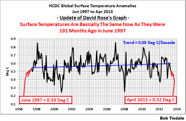
In his RMS article, Kevin Trenberth also conveniently overlooked the fact that the discussions about the warming halt are now for a time period of about 16 years, not 10 years—ever since David Rose’s DailyMail article titled “Global warming stopped 16 years ago, reveals Met Office report quietly released… and here is the chart to prove it”. In my response to Trenberth’s article, I updated David Rose’s graph, noting that surface temperatures in April 2013 were basically the same as they were in October 1997. We’ll use October 1997 as the start month for the running 17-year trends. The period is now 209-months long. The following graph is similar to the one above, except that it’s presenting running trends for 208-month periods.

Figure 7 – 209-Month Linear Trends
The last time global surface temperatures warmed at this low a rate for a 209-month period was the late 1970s, or about 1980. Also note that the sharp decline is similar to the drop in the 1940s, and, again, as you’ll recall, global surface temperatures remained relatively flat from the mid-1940s to the mid-1970s.
The most widely used metric of global warming—global surface temperatures—indicates that the rate of global warming has slowed drastically and that the duration of the halt in global warming is unusual during a period when global surface temperatures are allegedly being warmed from the hypothetical impacts of manmade greenhouse gases.
COMPARISONS
The GISS, HADCRUT4 and NCDC global surface temperature anomalies and the RSS and UAH lower troposphere temperature anomalies are compared in the next three time-series graphs. Figure 8 compares the five global temperature anomaly products starting in 1979. Again, due to the timing of this post, the HADCRUT4 and NCDC data lag the UAH, RSS and GISS products by a month. The graph also includes the linear trends. Because the three surface temperature datasets share common source data, (GISS and NCDC also use the same sea surface temperature data) it should come as no surprise that they are so similar. For those wanting a closer look at the more recent wiggles and trends, Figure 9 starts in 1998, which was the start year used by von Storch et al (2013) Can climate models explain the recent stagnation in global warming? They, of course, found that the CMIP3 (IPCC AR4) and CMIP5 (IPCC AR5) models could NOT explain the recent halt in warming.
Figure 10 starts in 2001, which was the year Kevin Trenberth chose for the start of the warming halt in his RMS article Has Global Warming Stalled?
Because the suppliers all use different base years for calculating anomalies, I’ve referenced them to a common 30-year period: 1981 to 2010. Referring to their discussion under FAQ 9 here, according to NOAA:
This period is used in order to comply with a recommended World Meteorological Organization (WMO) Policy, which suggests using the latest decade for the 30-year average.

Figure 8 – Comparison Starting in 1979
###########

Figure 9 – Comparison Starting in 1998
###########

Figure 10 – Comparison Starting in 2001
For those who want to get a rough idea of the impacts of the adjustments to the GISS and HADCRUT4 warming rates, refer to the July update—a month before those adjustments took effect.
AVERAGE
Figure 11 presents the average of the GISS, HADCRUT and NCDC land plus sea surface temperature anomaly products and the average of the RSS and UAH lower troposphere temperature data. Again because the HADCRUT4 and NCDC data lag one month in this update, the most current average only includes the GISS product.

Figure 11 – Average of Global Land+Sea Surface Temperature Anomaly Products
The flatness of the data since 2001 is very obvious, as is the fact that surface temperatures have rarely risen above those created by the 1997/98 El Niño in the surface temperature data. There is a very simple reason for this: the 1997/98 El Niño released enough sunlight-created warm water from beneath the surface of the tropical Pacific to permanently raise the temperature of about 66% of the surface of the global oceans by almost 0.2 deg C. Sea surface temperatures for that portion of the global oceans remained relatively flat until the El Niño of 2009/10, when the surface temperatures of the portion of the global oceans shifted slightly higher again. Prior to that, it was the 1986/87/88 El Niño that caused surface temperatures to shift upwards. If these naturally occurring upward shifts in surface temperatures are new to you, please see the illustrated essay “The Manmade Global Warming Challenge” (42mb) for an introduction.
MONTHLY SEA SURFACE TEMPERATURE UPDATE
The most recent sea surface temperature update can be found here. The satellite-enhanced sea surface temperature data (Reynolds OI.2) are presented in global, hemispheric and ocean-basin bases. We discussed the recent record-high global sea surface temperatures and the reasons for them in the post On The Recent Record-High Global Sea Surface Temperatures – The Wheres and Whys.
Thank you, this is good stuff.
Bob T, thank you for the excellent overall summary. Even completely accepting the mean of the surface and satellite record, the C in CAGW is clearly MIA. Indeed, as your linked charts point out, the A is difficult to find, and the GW is well below the model Mean, and likewise missing for at least ten years.
Yet the benefits of CO2 fertilization, well documented in the NIPCC reports, continue unabated. I think you are correct, the alarmist will present “any” warming as proof of future disaster (ignoring their failed model predictions which are based on wrong models depicting a great deal more warming then reality) and demand carbon tax schemes that do nothing to affect the GAT, but greatly harm the poor, and damage global economies.
Pre satellite data, and adjustments to the record bring into question the veracity of the “official” record during that “pre-satellite” time period. In the official record, as you note. “…and as you’ll recall, global surface temperatures remained relatively flat from the mid-1940s to the mid-1970s”, is in my view an assertion that likely, due to many adjustments, not reflect the reality of global T during that time.
Please remember that there were dozens of predicted fears that we were entering an ice age in the early to mid 1970s, Global GAT charts from that time period showed a great deal of cooling, not almost flat GAT changes. As documented here..http://stevengoddard.wordpress.com/1970s-ice-age-scare/ ” Every major climate organization endorsed the ice age scare, including NCAR, CRU, NAS, NASA – as did the CIA”
The cooling from the very warm late 1930s to early 1940s has been adjusted out to the data sets,
http://stevengoddard.wordpress.com/data-tampering-at-ushcngiss/
Indeed, long time politicians like Jerry Brown, governor in Calif during the 70s, then blamed droughts and fires on global cooling, and since re-elected as the current Governor, now blames droughts and cooling on global warming) Politicized scientists followed suit, blaming the cooling world for causing the polar vortex, which they now blame on CAGW.
http://stevengoddard.wordpress.com/2014/11/13/jerry-browns-1977-global-cooling-bs-recycled-as-jerry-browns-2014-global-warming-bs/
These adjustments go far beyond the TOB adjustments, and are in fact continuing now. I have challenged Mr. Mosher to explain even one of the adjustments shown at the below link for Iceland, where the local meteorologist disputes those adjustments.. UHI is likely well under represented as well. Documented history of adjustments here… http://stevengoddard.wordpress.com/data-tampering-at-ushcngiss/
Further support for RSS is that RSS follows the raw NCDC data very well. http://stevengoddard.wordpress.com/2014/10/15/why-i-trust-rss/
http://stevengoddard.wordpress.com/2014/10/16/why-i-trust-rss-part-2/
and the raw data tracks the recorded highs, which are not subject to TOB adjustments very well as well.
In summary, an accurate reflection of the warm early 1940s, would make the already very bad models, far worse, and maybe through abundant and inexpensive energy, we could better combat real problems, real pollution, and improve economies on a global basis.
“Indeed, long time politicians like Jerry Brown, governor in Calif during the 70s, then blamed droughts and fires on global cooling”
I looked through Steve Goddard’s post, and couldn’t see anywhere that Brown spoke of global cooling.
Correction to above post. “Indeed, long time politicians like Jerry Brown, governor in Calif during the 70s, then blamed droughts and fires on global cooling, and since re-elected as the current Governor, now blames droughts and FIRES on global warming.
Bob, great post as always and I did buy your book the other day. Just waiting for some free time to sit down and understand it.
Your Figure 6 has me confused in light of your “absence of warming” title and the text directly below the figure. If the anomalies are in deg/decade and they are all above 0.0 this means the period from 1980 to present has warmed virtually every year. What has happened recently is the rate of warming has dropped to the same value it was in 1980 (but still positive). So we are still warming based on the graph, no? Or am I out a derivative here?
You’re right, Steve from Rockwood. I’ll have to correct the boilerplate to read slowdown in the warming rate.
Had this been done for GISS for a 10 year period last month instead of 13 years, it would have gone to 0. But with the October numbers, there is no longer a flat period if I am not mistaken.
Reblogged this on Canadian Climate Guy.
October 2014 Global Surface (Land+Ocean) and Lower Troposphere Temperature Anomaly & Model-Data Difference Update.
All these different graphs by different people showing different things!
There should be just one final graph at the end of any paper or calculations and that is of global mean surface temperatures in real absolute terms. Everything else just confuses the issue!
“The causes of the changes are unclear at present, but they will likely affect the 2014 rankings at year end”.
Every little bit helps?
After 10 months, the GISS average is 0.664. The previous yearly high was 2010 at 0.661. 2005 is next at 0.655. GISS no longer shows a flat pause.
Hadcrut4.3, after 9 months, is 0.560. This is slightly above the record of 0.555 in 2010. After 9 months, the pause is 9 years and 9 months.
Hadsst3, at 0.482 after 10 months, is way ahead of 0.416 from 1998. The last 5 months have all been above the previous high monthly anomaly of 0.526 set in July 1998. It also no longer shows a pause.
The satellite data show pauses with RSS at 18 years and 1 month and UAH, version 5.5, at 9 years and 10 months. Both are ranked 7th after 10 months in 2014.
GISS has recently had a small adjustment all the way back to 1880. More than half the months up until about 1960 cooled, mostly by 0.01 deg C, and a few a little more. Since 1960, about half the months have warmed by 0.01 deg C. It has only a minimal effect on the overall trend, which is above zero all the way through. Two more months like September and October will make 2014 the warmest year in th 135 year record.
Werner – the latest version of UAH is 5.6, and this shows a slight cooling trend only as far back as October 2008
Thank you. I wish WFT would update UAH and Hadcrut4.3. It now stops in July when Hadcrut4.2 stopped. As well, there has been no WTI since May.
Hello Werner
You obviously follow these datasets very closely. You can easily work out your own trends, etc. with the help of Excel. If you email me at richardbarraclough2@gmail.com I can take you through it step by step, and then you won’t have to wait for WFT to do their updates.
Regards
Richard
Does the North Atlantic is warm? Svalbard freezes.
http://www.ijis.iarc.uaf.edu/seaice/data/201411/AM2SI20141114IC0.png
Thanks for the update Bob.
Your figure 1 struck me again as showing the post-Pinatubo rebound as an exponential relaxation to the new increased SW making it through the stratosphere.
I show the clear impact of the two major volcanoes on the stratosphere here:
http://climategrog.files.wordpress.com/2014/04/uah_tls_365d.png
Taking the same TLS data and applying a 365 day exponentially decaying relaxation ( no other low-pass filter used ) we see the strong similarity to GISS LOTI surface temp. anomaly.
http://climategrog.files.wordpress.com/2014/11/giss_loti_tls.png
The one year time constant is just a quick estimation that provides some lag for the ocean temps to react. TLS reacts very quickly to changes in forcing due to its negligible mass. This is also kept shorter than may be optimal best fit to avoid loosing too much of the start of the record Since we already lost the initial drop after El Chichon.
That was a bit brief, TLS cools as it becomes less opaque and more energy gets to lower climate. Explained more here:
http://climategrog.wordpress.com/?attachment_id=902
The bottom line is that the models run off because the warming was caused by stratospheric changes induced by the volcanoes, not GHG.
The surface warmed and climate had adjusted to a new equilibrium with the increased incoming solar energy by around 2000-2003. No more large volcanic disturbance is why there has be a “pause”. The TOA energy budget has remained fairly stable since.
The hypothesised attribution to GHG was a mistake: false attribution due to a spurious correlation. In fact the warming was volcanic in origin. Recognising and correcting that mistake is one of the biggest challenges facing this and future generations ™
Greg I looked at your posts and they are excellent. They show a 1.8 W per sq. M increased through-put to the surface of SW radiation driving the oceans, which clearly drive the GAT. Does anyone dispute this decrease in LT opacity allowing greater insolation to the oceans?
Sorry Greg, Does anyone dispute this decrease in TLS opacity allowing greater insolation to the oceans?
Thanks David, the 1.8 W/m2 is top of atmosphere SW energy budget for ERBE. I think that is generally accepted and non controvertion, but since stratosphere is cooling this must me making it in to the lower climate system.
Atmospheric optical density ( AOD ) data shows the change opacity and I don’t think that is generally a contested measurement. There have been several attempts to work out how much radiative forcing is caused by changes in AOD, basically Hansen et al trying to rig the data to get the models to work. However, that does not change the AOD data.
Ozone is one key factor here and there is some clear signs of step like changes in osone after the eruptions. NCAR recognise that step like changes and it is also mentioned in AR5.
I just don’t think anyone has really joined the dots yets. Or perhaps more likely does not want to break cover and say what the implications are.
They wil try to drag this out and take about 10 years to recognise it in the hope of milking the AGW cow until they retire.
Greg Goodman,
Very interesting. In what way is ozone a key factor, please tell.
I believe the “match” between the models and observations can be found only during the temperature data period used to “tune” the models. Prior to and after this tuning period the models do not match. It would be useful to add markers on your graph that identify this “tuning” period during which the models actually can’t be wrong because the observed temperature detailed input forces them to shadow observations. Models are then asked to hindcast and forecast the period before and the period after this section of time.
Given this tuned and therefore matched condition, it can be said, and clearly based on Bob’s model/observation differences graph, that the models cannot accurately hind or forecast climate outside of the tuned period. Nonetheless, trillions of dollars world wide has been spent on efforts to mitigate a future climate understood by even AGW scientists, to be simply a “scenario” based on one particular hypothesis of how climate works and now shown to be incorrect. The hypothesized scenario, as modeled, is a scenario that does not adequately explain the nature of climate. Case closed.
Needless to say, I want to know if any of my tax dollars are still being spent to allow these models to continue their unhelpful results and that allow scientists to continue to study the results of these incorrect scenario outcomes. I want names of those in the hallowed halls of government who fund the life line of money that keep these models alive and fund scientists who suckle at the teat of these very expensive computers.
Pamela, I believe the “match” between the models and observations can be found only during the temperature data period used to “tune” the models.”
I also think that to some degree the temperature data was tuned to the models. http://wattsupwiththat.com/2014/11/15/october-2014-global-surface-landocean-and-lower-troposphere-temperature-anomaly-model-data-difference-update/#comment-1789816
Pamela: if you look at the IPCC figure 9.8 from the latest IPCC Assessment Report representing all models currently used you find with just you eyes as a validation instrument exactly what you write: the best “match” takes place in the yellowish ~1960-1990 zone representing the reference period used for setting the mean T anomaly at zero
See it: http://climate.mr-int.ch/index.php/en/modelling-uk/other-models-uk
Smoothing data series don’t change the underlying phenomena, but, may be, eliminate short term perturbations.
The tougher question is to identify long term trends from short term identified perturbations and on-going identified cyclic variations.
It seems to me somehow futile to argue about monthly averages among various methods of data massaging over the past few decades, when the climates (plural) may slightly change over centuries.
Some parameter separation can be obtained by multi-variate regression analysis. However, lacking long term data series, the results are only partial and unsatisfactory.
This is why models are developed: to overcome the unavailability of the relevant data series. But they produce not very convincing in silico fictions. All but one models reviewed by IPCC in its 5th Assessment report overestimate the current average Temperature anomaly. (see fig 9.8).
¿ por qué será ?
Model validation is a key question because scenarios evaluated with failed modelsare just garbage.
¿ por qué será ?
because volcanoes: see above.
“This is why models are developed: to overcome the unavailability of the relevant data series. ”
If you don’t have data you can’t make a meaningful model. End of storey.
https://twitter.com/BigJoeBastardi
How do you explain the difference Bob? I say NCDC and GISS data amongst others is manipulated. I do not believe it.
Which of Joe Bastardi’s tweets are you referring to, Salvatore Del Prete. BTW, I’m only presenting data.
http://models.weatherbell.com/climate/ncep_cfsr_t2m_anom_ytd.png
How is this reconciled?
I’d be happy to reply if you’d please provide a workable link, Salvatore Del Prete. The webpage you linked is only available to WeatherBell subscribers.
Sure looks to me that the “hiatus” if it ever existed is over! http://ds.data.jma.go.jp/tcc/tcc/products/gwp/temp/oct_wld.html
The link shows a series of monthly graphs of global temperature with a superimposed linear trend line of 0.6 – 0.8C/ century. If true , and I personally have no evidence to refute the results , is that really a tragedy or a catastrophe? Does it really justify the removal of billions or even possibly trillions of dollars from the working families of the US and Europe, and the effect that that will have on the health of economies which depend on cash circulating between producer and consumer.
At the end of the day did not Clinton have it right on the button : ” it is the economy, stupid”.
You like October. Can I choose February instead?
I see the reference number is different for example GISS goes from 1951-1980 and the data near the poles is treated differently. I get it .
What I still don’t get is why Weatherbell’s data is lower then UAH data? UAH data for year 2014 through Oct shows a temperature deviation much higher then the .11c Weatherbell has and they use the same reference number of years 1981-2010.
Thanks, Bob. Your brilliant vision of the oceans is much appreciated.
This temperature plateau will most surely be terminated by ENSO, which brought us were we are now.
UAH deviation through OCT +.261 c Weather bell +.11c through NOV 05 .
Which one is most correct I do not know but both I feel are not biased and the best temperature data out there and I blend the two of them.
Good work, yes.
The take-away I get: currently models (and simplistic projections of prior temperature rise rates) are about 0.2C warmer than observations. that is 50% too warm (not 0.6 but 0.4C change since 1975). The disconnect will be getting greater and faster as the CO2 rises.
The amount of energy “missing”: would be delta 0.2 X the heat capacity of air X the mass of the atmosphere?
We are at the end of a 30 year warm cycle. When graphs begin in 1979, key cold year, it looks like it is ‘warmer and warmer!’ but already it is getting much colder. We don’t look at the US West Coast to see if we have global cooling, we look at Antarctica and the places where there is always a mile high glacier sheet every Ice Age, namely most of North America down to below the Great Lakes and all of New England and of course, Europe. Not Africa or Australia or even Siberia that also had no huge ice sheets during any Ice Age.
It is cold now in the key areas! Dreadfully cold. I don’t care how warm it is in Portland, Oregon or Mali, Africa. It is how cold is it in the glacier belt!
Has anyone correlated the temperature rise over the 20th century with rainfall and crop production? Surely one of the potential catastrophies inherent in CAGW will be an inability to feed people and provide water. Yet somehow the population has grown from 1.7 billion in 1900 to 7 billion today, and energy consumption has grown from 40 exajoules per year to 540. Since 1960 food production per capita has grown from 310 to 390 kgs per year.
So to date it would appear that about 1 degree of global warming has had no detrimental effects on people.
But I can hear the alarmists crying – just you wait, we are all doomed. And if we keep focusing on the wrong things, they will eventually be proved correct. The issues will be population and resources.
Bob – you seem blissfully unaware that your figures 1, 2, and 3 (that is GISS, HadCRUT & NCDC) are riddled with computer noise in the form of sharp upward spikes. One such spike makes the super El Nino peak at 1998 0.2 degrees higher than it is. There are ten or more such spikes in each graph. They are located in exactly the same places, namely beginnings of years, and this eliminates the possibility of random noise. It was obviously a secret operation but they screwed up and did not realize that the computer was leaving its footprints in publicly available data sets. You with your facility for temperature curves ought to be able to clean one up and show us what temperature looked like before and after removal of noise.
Arno Arrak, says, “It was obviously a secret operation…”
Thanks for the conspiracy theory, Arno.
“That boy could be President!” (“The Grifters”)
Bob
I respect the work you put into this, but really, try looking at your own report objectively.
Comparing temperature trends with models is clearly interesting, but does not negate real warming. Its a bit like saying “I expected to climb the stairs in 6 seconds but it took 8”. You still climbed the stairs.
Your statement that
“Alarmists happily ignore the fact that it is easy to have record high global temperatures in the midst of a hiatus or slowdown in global warming”
is simply a contortion.
Record high temperatures, be they after a 2 year pause or a 12 year pause are still record high if they pass the previous highest level. Its not “easy”, its just a fact. And that fact must be a massive thorn in the side of all those who stated, so vociferously but without a shred of evidence, that in the near-term there would no more warming, that there would be cooling, or even predicting a mini ice age.
Looking at the evidence you present, I would suggest it says:
Warming continues but as expected its not linear over short periods. It appears to be following step changes, with lulls in between. It appears that we may be in an upward step now, that started a few years ago, but its too early to be sure. Clearly we are now at a higher “base” level than we were in the late 1990’s, when it is claimed the current pause started. Actually the pause started about 2002, but now looks to be coming to an end. Overall since 1980, the rate of warming is in the range 0.12 C to 0.16 C per decade.
.
Hi James, my statement “Alarmists happily ignore the fact that it is easy to have record high global temperatures in the midst of a hiatus or slowdown in global warming” is not a contortion. Depending on the dataset, there had been record high annual surface temperatures during the hiatus, yet the hiatus persisted.
I don’t know what will happen next year or the year after. Do you?
You closed with, “Overall since 1980, the rate of warming is in the range 0.12 C to 0.16 C per decade.”
But the hiatus refers to a shorter timespan, so I’m not sure why you’d attempt to change the term being discussed.
Regards
James.
As you fall off the top of a high amplitude sine-wave, the readings you get are all still high, even if you are plummeting like a stone.
This is doubly true, if you start the linear trend at the bottom of the sine wave (ie, the 1970s). By doing this, you will always have an upwards linear trend, all the way until you reach the bottom of the sine-wave again. If climate is running to a PDO-style 60-year sine wave, then if you start the linear comparison in 1970, you will not reach a zero trend until 2030.
Plenty of time to go, James. Plenty of time.
Ralph
If only it were as warm out as some people here are saying! I go outside these days – and it’s cold! Noticeably colder here (to the east of the North Atlantic) than it was ten years ago. I was in the northeastern US late this summer and was told that they had had only one day above 90 degrees state. That didn’t happen ten years ago, either. So I conclude that either the North Atlantic area has detached itself from the world climate system – or someone’s cooking the books, just like Steve Goddard is saying.
James Abbott,
We are nowhere near ‘record high temperatures’. Geologically, we are on the cold side of global temperatures. Even recently, during the Holocene, global T was considerably higher than now.
The planet has been recovering from the LIA — one of the coldest episodes of the Holocene. I suspect it will continue to recover, after we go thru a cooling phase.
What I do know is that there is still no measurable evidence that human emissions are the cause of global warming. I will listen to any evidence you have. But without testable evidence, it’s belief. Skeptics need more than belief.
dbstealey
Moving the goalposts does not work – we can see you doing it.
Clearly, I was referring to Bob’s report and clearly to his plots of measured temperatures starting in the late 1970s.
So if you want to talk about it being warmer in the geological past when there were no human GHG influences, then yes you are bang on correct, buts that’s not the period we are talking about.
There is plenty of evidence that the current warming is likely to be linked to changes in GHG concentrations that humans have caused. You simply do not want to know about it because your mind is closed.
Firstly, the observed warming cannot be sensibly explained by other mechanisms. Secondly, the extent and timing of the observed warming is commensurate with that expected from calculating the enhanced GHE (albeit currently rather less than expected).
Finally, you state that
“The planet has been recovering from the LIA — one of the coldest episodes of the Holocene. I suspect it will continue to recover, after we go thru a cooling phase.”
Actually the evidence suggests that the LIA was an episode within a longer term cooling trend – and that the recovery from the LIA episode is long gone.
But I like your comment that you “suspect” what the future holds. Sounds about as robust as reading the tea leaves there.
“rather less”? If by “rather less”, you mean ‘travesty’, then I agree with you.