Guest essay by Ken Gregory
See abstract and PDF version here.
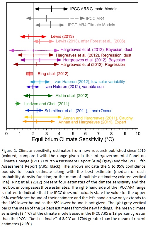
The determination of the global warming expected from a doubling of atmospheric carbon dioxide (CO2), called the climate sensitivity, is the most important parameter in climate science. The Intergovernmental Panel on Climate Change (IPCC) fifth assessment report (AR5) gives no best estimate for equilibrium climate sensitivity “because of a lack of agreement on values across assessed lines of evidence and studies.”
Studies published since 2010 indicates that equilibrium climate sensitivity is much less that the 3 °C estimated by the IPCC in its 4th assessment report. A chart here shows that the mean of the best estimates of 14 studies is 2 °C, but all except the lowest estimate implicitly assumes that the only climate forcings are those recognized by the IPCC. They assume the sun affects climate only by changes in the total solar irradiance (TSI). However, the IPCC AR5 Section7.4.6 says,
“Many studies have reported observations that link solar activity to particular aspects of the climate system. Various mechanisms have been proposed that could amplify relatively small variations in total solar irradiance, such as changes in stratospheric and tropospheric circulation induced by changes in the spectral solar irradiance or an effect of the flux of cosmic rays on clouds.”
Many studies have shown that the sun affects climate by some mechanism other than the direct effects of changing TSI, but it is not possible to directly quantify these indirect solar effects. All the studies of climate sensitivity that rely on estimates of climate forcings which exclude indirect solar forcings are invalid.
Fortunately, we can calculate climate sensitivity without an estimate of total forcings by directly measuring the changes to the greenhouse effect.
The greenhouse effect (GHE) is the difference in temperature between the earth’s surface and the effective radiating temperature of the earth at the top of the atmosphere as seen from space. This temperature difference is generally given as 33 °C, where the top-of-atmosphere global average temperature is about -18 °C and global average surface temperature is about 15 °C. We can estimate climate sensitivity by comparing the changes in the GHE to the changes in the CO2 concentrations.
The Clouds and Earth’s Radiant Energy System (CERES) experiment started collecting high quality top-of-atmosphere outgoing longwave radiation (OLR) data in March 2000. The last data available is June 2013 as of this writing on January 14, 2013. Figure 1 shows a typical CERES satellite.

Figure 1. CERES Satellite
The CERES OLR data presented by latitude versus time is shown in Figure 2.

Figure 2. CERES Outgoing Longwave Radiation, latitude versus date.
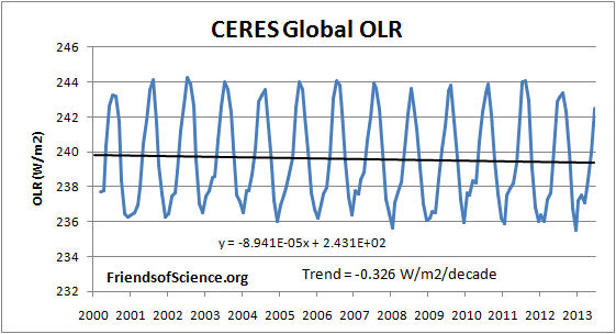
The global average OLR is shown in Figure 3.

Figure 3. CERES global OLR.
The CERES OLR data is converted to the effective radiating temperature (Te) using the Stefan-Boltzmann equation.
Te = (OLR/σ)0.25 – 273.15. where σ = 5.67 E-8 W/(m2K4), Te is in °C.
The monthly anomalies of the Te were calculated so that the annual cycle would not affect the trend.
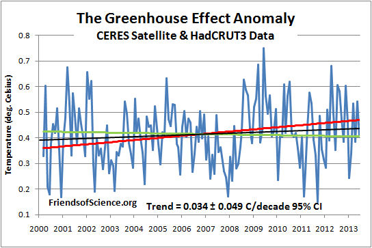
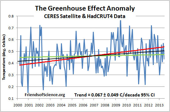
We use the HadCRUT temperature anomaly indexes to represent the earth’s surface temperature (Ts). The HadCRUT3 temperature index shows a cooling trend of -0.002 °C/decade, and the HadCRUT4 temperature index shows a warming trend of 0.031 °C/decade during the period with CERES data, March 2000 to June 2013. The land measurement likely includes a warming bias due to uncorrected urban warming. The hadCRUT4 dataset added more coverage in the far north, where there has been the most warming, but failed to add coverage in the far south, where there has been recent cooling, thereby introducing a warming bias. We present results using both datasets.
The difference between the surface temperatures anomaly and effective radiating temperature anomaly is the GHE anomaly. Figures 4 and 5 show the Greenhouse effect anomaly utilizing the HadCRUT3 and HadCRUT4 temperature indexes, respectively.

Figure 4. The greenhouse effect anomaly based on CERES OLR and HadCRUT3.

Figure 5. The greenhouse effect anomaly based on CERES OLR and HadCRUT4.
The trends of the GHE are 0.0343 °C/decade based on HadCRUT3, and 0.0672 °C/decade based on HadCRUT4.
We want to compare these trends in the GHE to changes in CO2 to determine the climate sensitivity. Only changes in anthropogenic greenhouse gases can cause a significant change in the greenhouse effect. Changes in the sun’s TSI, aerosols, ocean circulation changes and urban heating can’t change the GHE. Changes in cloudiness could change the GHE, but data from the International Satellite Cloud Climatology Project shows that the average total cloud cover during the period March 2000 to December 2009 changed very little. Therefore, we can assume that the measured change in the GHE is due to anthropogenic greenhouse gas emissions, which is dominated by CO2.
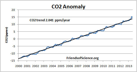
The CO2 data also has a large annual cycle, so the anomaly is used. Figure 6 shows the monthly CO2 anomaly calculated from the Mauna Loa data and the best fit straight line.

Figure 6. CO2 anomaly.
The March 2000 CO2 concentration is assumed to be the 13 month centered average CO2 concentration at March 2000, and the June 2013 value is that value plus the anomaly change from the fitted linear line. Table 1 below shows the CO2 concentrations, the logarithm of the CO2 concentration, and the change in the GHE from March 2000 for both the HadCRUT3 and HadCRUT4 cases.
Table 1 shows that the GHE has increased by 0.046 °C from March 2000 to June 2013 based on changes in the CERES OLR data and HadCRUT3 temperature data. Extrapolating to January 2100, the GHE increase to 0.28 °C by January 2100. Using the HadCRUT4 temperature data, the GHE increases by 0.55 °C by January 2100 compared to March 2000.
| hadCRUT3 | hadCRUT4 | |||
| Date | CO2 | Log CO2 | ΔGHE | ΔGHE |
| ppm | °C | °C | ||
| March 2000 | 368.88 | 2.567 | 0 | 0 |
| June 2013 | 395.94 | 2.598 | 0.046 | 0.089 |
| January 2100 | 572.68 | 2.758 | 0.283 | 0.554 |
| 2X CO2 | 737.76 | 2.868 | 0.446 | 0.873 |
Table 1. Extrapolated changes to the greenhouse effect (GHE) based on two versions of the hadCRUT datasets.
Table 1 shows that the GHE has increased by 0.046 °C from March 2000 to June 2013 based on changes in the CERES OLR data and HadCRUT3 temperature data. Extrapolating to January 2100, the GHE increase to 0.28 °C by January 2100. Using the HadCRUT4 temperature data, the GHE increases by 0.55 °C by January 2100 compared to March 2000.
The last row of Table 1 shows the transient climate response (TCR), which is the temperature response to CO2 emissions from March 2000 levels to the time when CO2 concentrations have doubled. TCR is less than the equilibrium climate sensitivity because the oceans have not reached temperature equilibrium at the time of CO2 doubling. TCR is calculated by the equation:
TCR = F2x dT/dF ; where dT means the temperature difference, dF means the forcing difference, from March 2000 to June 2013.
The CO2 forcing was calculated as 5.35 x ln (CO2/CO2i). The change in forcing from March 2000 to June 2013 is 0.379 W/m2. The forcing for double CO2 (F2x) is 3.708 W/m2. The TCR is 0.45 °C using hadCRUT3, and 0.87 °C using hadCRTU4 data. These values are much less than the multi-model mean estimate of 1.8 °C for TCR given in Table 9.5 of the AR5. The climate model results do not agree with the satellite and surface data and should not be used to set public policies.
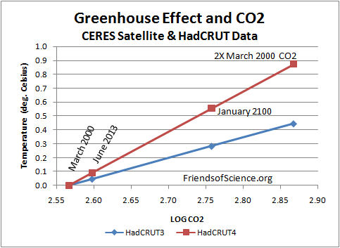
Figure 7 shows the results of Table 1 graphically.

Figure 7. The greenhouse effect and CO2 extrapolated to January 2100 and double CO2 bases on CERES and HadCRUT data.
This analysis suggests that the temperature change from June 2013 to January 2100 due to increasing CO2 would be 0.24 °C (from HadCRUT3) or 0.46 °C (from HadCRUT4), assuming the CO2 continues to increase along the recent linear trend.
An Excel spreadsheet with the data, calculations and graphs is here.
HadCRUT3 data is here.
HadCRUT4 data is here.
Mauna Loa CO2 data is here.
CERES OLR data is here.
Total cloud cover data is here.
lgl
This is a bit confused
blockquote> 60% and 2.5 amplification is the same thing. If you add 60% of the output of a closed feedback loop to the input, the resulting gain is 2.5. [G=1/1-0.6] This of course being the amplification of the solar input to the surface and not amplification of the surface radiation.
In terms of heating at the surface it is the GAIN that is 60% not the Feedback, i.e. 390/240 = ~1.6
Re-working your numbers for a 3.7 w/m2 TOA reduction in albedo (not sure exactly what this means). Surface radiation increases by ~6.2 w/m2. Temp increases are 0.98k and 1.13k for TOA and surface respectively. So a ~0.05k anomaly for a pretty hefty reduction (equivalent to doubling CO2) in albedo.
John
But this is taken into account by using Ts-Te
Not when he is assuming all the change in GHE is due to CO2.
You can’t do the calcs like that. The increased forcing will also increase the GHE (more vapor) but even your method gives 0.15K or 15% (not 0.05)
He’s not he’s calculating the enhanced greenhouse effect. However, CO2 is the primary driver without which there would be no feedback (according to the climate scientists).
Yep. The total additional GH forcing (2000-2013) being that inferred from the Ts-Te trend.
My mistake but not really relevant to the past 13 years because any temperature increase is so small. The Hadcrut4 trend is 0.031 deg per decade. Whatever I ‘m sure Ken Gregory won’t worry too much about a 15% increase to the Ts-Te trend.
lgl says:
The equation is: TCR = F2x X d(Ts-Te)/dF,
where dF means the forcing difference that could cause the change of (Ts-Te), from March 2000 to June 2013.
My previous comment shows from line-by-line computer code, without feedbacks, a 1 C change in causes a 0.97 C change in OLR, therefore, without feedbacks, dF only includes forcings that change the longwave absorbtion. However, during the period of analysis, there was no temperature change, with HadCRUT3 showing an insignificant decline, HadCRUT4 showing an insignificant rise. With no temperature change there is no feeback, so no water vapor change.
Therefore, dF includes only changes in greenhouse gases and potentially a longwave component of cloud changes. But clouds have a large shortwave effect and only a small longwave effect. Over the period of analysis there was only a tiny change in total clouds. Therefore, dF includes only changes in greenhouse gases, and this dF is known.
there was no temperature change
because the added CO2 prevented the drop a weaker ENSO would have caused.
@RACookPE1978….”””””……BUT – the open ocean albedo for direct radiation is very, very different: At high SEA angles near noon at the equator, it is about 0.05, but then increases significantly as SEA approaches the horizon, until albedo is measured at 0.35 to 0.40 at the horizon. (Some sources measure albedo even higher, but these are the best averages for all open waters. Thus, at low solar elevation angles each morning and evening at all latitudes, approximately 40% of the sun’s direct energy is reflected from the ocean – 7 to 8 times what is reflected at noon…….”””””””
These numbers are quite misleading. Also, it would be better to talk of incidence angles (zenith angle) rather than morning, noon, and evening.
Over the bulk of the solar spectrum (energy wise) the reflectance of water at normal incidence (zenith sun) is easily calculated at 2% ; not 6% so 98% of the sea surface incident solar energy would be absorbed, not 94%.
But it can also be calculated from the full polarized Fresnel reflection formulae, that the total reflectance of both polarizations is almost constant up to the Brewster angle of incidence, which for water is easily shown to be about 53.1 degrees.
Thus, the sea surface reflectance for both specular sun and diffuse sky irradiance, is still about 2% out to about 53 degrees INCIDENCE angle. Because of atmospheric refraction lowering the apparent sun zenith angle (slightly), the actual sun angle is greater than 53.1. Refraction lifts the sun by more than its diameter, at the horizon, so when the apparent sun makes first contact with the horizon, the sun is already more than a half degree below the horizon.
But I’ll stay with the 53 degrees.
On the equator, at the equinoxes, the sun spends over seven hours within 53 degrees of the zenith, with the sea surface transmitting 98% of the incident energy.
For the diffuse (assumed Lambertian) irradiance, the flux within that 53 degree cone is given by sin^2(53.1 deg.), which is fully 64% of the total flux. However, the diffuse radiation from the sunlit sky (clear sky) is clearly NOT Lambertian; it is highly biased towards the sun direction, So somewhat more than 64 % of the diffuse sunlight is contained in that 53 degree Brewster angle cone, that the sun spends up to seven hours in. Exact calculation is more complex, so I’ll leave it at 64%.
At 53.1 deg. zenith angle , the cosine is 0.6 (3,4,5 triangle), so whereas we have an air mass one (AM1) solar spectrum at the zenith, it is already AM1.667 at the Brewster angle , so the incoming atmospheric absorption of solar energy is greatly increased over the zenith absorption. The reflected 2% of the surface incident solar energy, at the Brewster angle, also faces an AM1.667 atmospheric absorption, on its way out, and that atmospheric absorbed solar energy, becomes part of the solar incident energy converted to diffuse LWIR by the atmosphere.
The long and the short of this is that early morning and late afternoon oblique solar energy, become an increasing component of the atmospheric LWIR emission, and a not very significant component of ocean surface albedo, either specular or diffuse.
The effect of the increased atmospheric path length absorption of solar energy, at sunrise and sunset, is so pronounced, that humans can look directly at the sun with impunity, at and near those times. even 35 or 40% reflection of the total surface incident irradiant solar energy, around those times, is a quite inconsequential contribution to the surface component, or earth’s albedo. it takes only an hour from sunrise, for the tropical sun to reach 15 degrees altitude; or 75 deg. zenith angle. at that point the effective atmospheric air mass is still AM3.86, so surface irradiance is still highly attenuated from the zenith value. Expanding a normal incidence ocean surface albedo from 0.020, to an integrated average of 0.06 over the whole surface to come up with a 94% ocean absorption, is plain fiction.
The famous earthrise photograph from the moon, from the Apollo landing, shows that the earth’s ocean surface, is completely invisible to the eye. Only the cloud cover, and the blue sky scattered light can be discerned over the ocean; the ocean surface itself is black, due to its almost total absorption of solar energy incident on it.
Ken Gregory says: January 18, 2014 at 11:34 am “Over the period of analysis there was only a tiny change in total clouds.”
That is an interesting statement as the Cloud cover data that Mr Gregory links to stops at December 2009, so he can’t factor in the last 4 years. As the period form 1986 to 2000 show a Decrease in cloud of about 5.8%, what happened after 2009, because by then it had already increased again by over 1.2%?
If you don’t believe me check out the link yourselves.
The other point is what emissivity value was used, Mr Esenbache said that for this kind of work the value of 1.0 was used, however the emissivity of Water is quoted as anything from 0.90 to 0.98.
That of course changes the initial value of around 400 W/m2 to at
0.98 = 392 W/m2
0.95 = 380 W/m2
0.90 = 360 W/m2