Guest essay by Ken Gregory
See abstract and PDF version here.
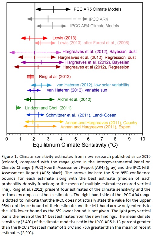
The determination of the global warming expected from a doubling of atmospheric carbon dioxide (CO2), called the climate sensitivity, is the most important parameter in climate science. The Intergovernmental Panel on Climate Change (IPCC) fifth assessment report (AR5) gives no best estimate for equilibrium climate sensitivity “because of a lack of agreement on values across assessed lines of evidence and studies.”
Studies published since 2010 indicates that equilibrium climate sensitivity is much less that the 3 °C estimated by the IPCC in its 4th assessment report. A chart here shows that the mean of the best estimates of 14 studies is 2 °C, but all except the lowest estimate implicitly assumes that the only climate forcings are those recognized by the IPCC. They assume the sun affects climate only by changes in the total solar irradiance (TSI). However, the IPCC AR5 Section7.4.6 says,
“Many studies have reported observations that link solar activity to particular aspects of the climate system. Various mechanisms have been proposed that could amplify relatively small variations in total solar irradiance, such as changes in stratospheric and tropospheric circulation induced by changes in the spectral solar irradiance or an effect of the flux of cosmic rays on clouds.”
Many studies have shown that the sun affects climate by some mechanism other than the direct effects of changing TSI, but it is not possible to directly quantify these indirect solar effects. All the studies of climate sensitivity that rely on estimates of climate forcings which exclude indirect solar forcings are invalid.
Fortunately, we can calculate climate sensitivity without an estimate of total forcings by directly measuring the changes to the greenhouse effect.
The greenhouse effect (GHE) is the difference in temperature between the earth’s surface and the effective radiating temperature of the earth at the top of the atmosphere as seen from space. This temperature difference is generally given as 33 °C, where the top-of-atmosphere global average temperature is about -18 °C and global average surface temperature is about 15 °C. We can estimate climate sensitivity by comparing the changes in the GHE to the changes in the CO2 concentrations.
The Clouds and Earth’s Radiant Energy System (CERES) experiment started collecting high quality top-of-atmosphere outgoing longwave radiation (OLR) data in March 2000. The last data available is June 2013 as of this writing on January 14, 2013. Figure 1 shows a typical CERES satellite.

Figure 1. CERES Satellite
The CERES OLR data presented by latitude versus time is shown in Figure 2.

Figure 2. CERES Outgoing Longwave Radiation, latitude versus date.
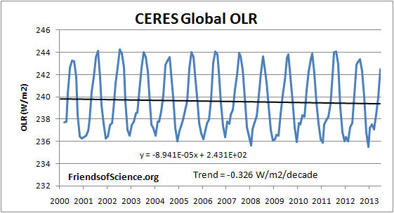
The global average OLR is shown in Figure 3.

Figure 3. CERES global OLR.
The CERES OLR data is converted to the effective radiating temperature (Te) using the Stefan-Boltzmann equation.
Te = (OLR/σ)0.25 – 273.15. where σ = 5.67 E-8 W/(m2K4), Te is in °C.
The monthly anomalies of the Te were calculated so that the annual cycle would not affect the trend.
We use the HadCRUT temperature anomaly indexes to represent the earth’s surface temperature (Ts). The HadCRUT3 temperature index shows a cooling trend of -0.002 °C/decade, and the HadCRUT4 temperature index shows a warming trend of 0.031 °C/decade during the period with CERES data, March 2000 to June 2013. The land measurement likely includes a warming bias due to uncorrected urban warming. The hadCRUT4 dataset added more coverage in the far north, where there has been the most warming, but failed to add coverage in the far south, where there has been recent cooling, thereby introducing a warming bias. We present results using both datasets.
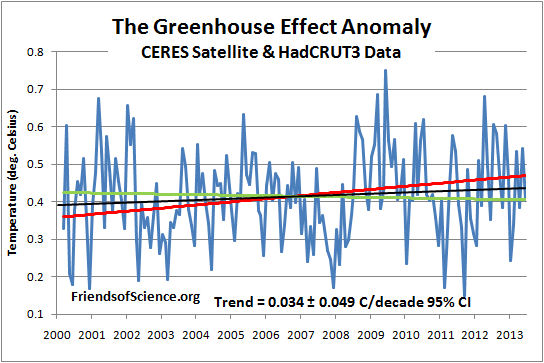
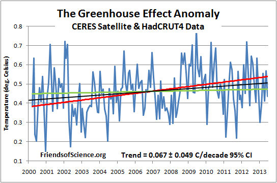
The difference between the surface temperatures anomaly and effective radiating temperature anomaly is the GHE anomaly. Figures 4 and 5 show the Greenhouse effect anomaly utilizing the HadCRUT3 and HadCRUT4 temperature indexes, respectively.

Figure 4. The greenhouse effect anomaly based on CERES OLR and HadCRUT3.

Figure 5. The greenhouse effect anomaly based on CERES OLR and HadCRUT4.
The trends of the GHE are 0.0343 °C/decade based on HadCRUT3, and 0.0672 °C/decade based on HadCRUT4.
We want to compare these trends in the GHE to changes in CO2 to determine the climate sensitivity. Only changes in anthropogenic greenhouse gases can cause a significant change in the greenhouse effect. Changes in the sun’s TSI, aerosols, ocean circulation changes and urban heating can’t change the GHE. Changes in cloudiness could change the GHE, but data from the International Satellite Cloud Climatology Project shows that the average total cloud cover during the period March 2000 to December 2009 changed very little. Therefore, we can assume that the measured change in the GHE is due to anthropogenic greenhouse gas emissions, which is dominated by CO2.
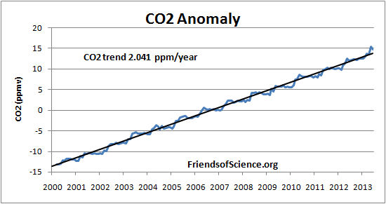
The CO2 data also has a large annual cycle, so the anomaly is used. Figure 6 shows the monthly CO2 anomaly calculated from the Mauna Loa data and the best fit straight line.

Figure 6. CO2 anomaly.
The March 2000 CO2 concentration is assumed to be the 13 month centered average CO2 concentration at March 2000, and the June 2013 value is that value plus the anomaly change from the fitted linear line. Table 1 below shows the CO2 concentrations, the logarithm of the CO2 concentration, and the change in the GHE from March 2000 for both the HadCRUT3 and HadCRUT4 cases.
Table 1 shows that the GHE has increased by 0.046 °C from March 2000 to June 2013 based on changes in the CERES OLR data and HadCRUT3 temperature data. Extrapolating to January 2100, the GHE increase to 0.28 °C by January 2100. Using the HadCRUT4 temperature data, the GHE increases by 0.55 °C by January 2100 compared to March 2000.
| hadCRUT3 | hadCRUT4 | |||
| Date | CO2 | Log CO2 | ΔGHE | ΔGHE |
| ppm | °C | °C | ||
| March 2000 | 368.88 | 2.567 | 0 | 0 |
| June 2013 | 395.94 | 2.598 | 0.046 | 0.089 |
| January 2100 | 572.68 | 2.758 | 0.283 | 0.554 |
| 2X CO2 | 737.76 | 2.868 | 0.446 | 0.873 |
Table 1. Extrapolated changes to the greenhouse effect (GHE) based on two versions of the hadCRUT datasets.
Table 1 shows that the GHE has increased by 0.046 °C from March 2000 to June 2013 based on changes in the CERES OLR data and HadCRUT3 temperature data. Extrapolating to January 2100, the GHE increase to 0.28 °C by January 2100. Using the HadCRUT4 temperature data, the GHE increases by 0.55 °C by January 2100 compared to March 2000.
The last row of Table 1 shows the transient climate response (TCR), which is the temperature response to CO2 emissions from March 2000 levels to the time when CO2 concentrations have doubled. TCR is less than the equilibrium climate sensitivity because the oceans have not reached temperature equilibrium at the time of CO2 doubling. TCR is calculated by the equation:
TCR = F2x dT/dF ; where dT means the temperature difference, dF means the forcing difference, from March 2000 to June 2013.
The CO2 forcing was calculated as 5.35 x ln (CO2/CO2i). The change in forcing from March 2000 to June 2013 is 0.379 W/m2. The forcing for double CO2 (F2x) is 3.708 W/m2. The TCR is 0.45 °C using hadCRUT3, and 0.87 °C using hadCRTU4 data. These values are much less than the multi-model mean estimate of 1.8 °C for TCR given in Table 9.5 of the AR5. The climate model results do not agree with the satellite and surface data and should not be used to set public policies.
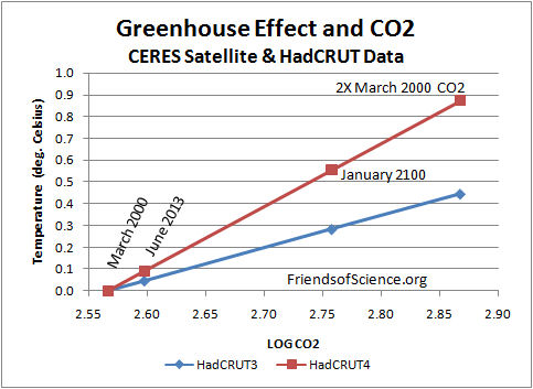
Figure 7 shows the results of Table 1 graphically.

Figure 7. The greenhouse effect and CO2 extrapolated to January 2100 and double CO2 bases on CERES and HadCRUT data.
This analysis suggests that the temperature change from June 2013 to January 2100 due to increasing CO2 would be 0.24 °C (from HadCRUT3) or 0.46 °C (from HadCRUT4), assuming the CO2 continues to increase along the recent linear trend.
An Excel spreadsheet with the data, calculations and graphs is here.
HadCRUT3 data is here.
HadCRUT4 data is here.
Mauna Loa CO2 data is here.
CERES OLR data is here.
Total cloud cover data is here.
Gregory says: January 16, 2014 at 1:40 pm
I haven’t done that. But I have now added the 95% confidence intervals to the two plots of the GHE vs time. On the article, click on the links “Figure 4” and “Figure 5” under the plots.
or
http://www.friendsofscience.org/assets/documents/CERES/GHE_Anomaly3.jpg
http://www.friendsofscience.org/assets/documents/CERES/GHE_Anomaly4.jpg
The 95% confidence was calculated as per;
http://people.stfx.ca/bliengme/ExcelTips/RegressionAnalysisConfidence2.htm
Ken Gregory:
re your post at January 16, 2014 at 4:17 pm.
Thankyou. As you are aware, it is a step towards what I recommended above.
Richard
Ken Gregory – you say “There is no such thing as reflected solar longwave radiation “. My understanding is that about a half of solar radiation is infrared …
[https://en.wikipedia.org/wiki/Infrared “Sunlight, at an effective temperature of 5,780 kelvins, is composed of nearly thermal-spectrum radiation that is slightly more than half infrared. At zenith, sunlight provides an irradiance of just over 1 kilowatts per square meter at sea level. Of this energy, 527 watts is infrared radiation, 445 watts is visible light, and 32 watts is ultraviolet radiation.“]
… and that infrared is regarded as longwave radiation [http://www.nasa.gov/audience/forstudents/5-8/features/F_Infrared_Light_5-8.html “Many things besides people and animals emit infrared light – the Earth, the Sun, and far away things like stars and galaxies do also!“].
I would also expect that ice and snow would reflect longwave, even if oceans don’t [NASA again: “We know that many things emit infrared light. But many things also reflect infrared light.“].
On ‘natural CO2 production’, I’m not talking about the annual cycle, I’m talking primarily about the ocean-atmosphere interface. This is, of course, where most of the ‘about half of man-made CO2 production’ goes. If there is an ocean-atmosphere CO2 imbalance then CO2 will flow between the two, but the act of flowing reduces the imbalance and therefore (all other things being equal) subsequent flow will be at a lesser rate. ie, the rate can change even if temperature does not. The imbalance has a half-life of around 12 years, so the rate would halve in about 12 years.
(Apologies for using Wikipedia and NASA ‘for students’ as references, but they put things simply. Wikipedia in non-contentious issues should be OK.)
higley7 says:
January 16, 2014 at 9:51 am
The surface of the Earth with no atmosphere would be the same as the moon, which is at 127 deg C in sunlight (-173 deg C on the dark side).
As climate models assume 24 hour a day sunlight, the 127 deg C temperature is applicable.
So, without an atmosphere, the Earth would be at 127 deg C at the surface and, instead, with an atmosphere is at 15 deg C. It is not a big stretch to see that the atmosphere clearly cools the planet’s surface, giving the surface more ways to shed heat, by conduction and convection, rather than just by radiation with no atmosphere.
Mike Jonas says:
January 16, 2014 at 5:36 pm
Plus the direct teaching of still traditional science on the subject from NASA:
Here is traditional teaching from direct NASA pages: http://science.hq.nasa.gov/kids/imagers/ems/infrared.html
“Far infrared waves are thermal. In other words, we experience this type of infrared radiation every day in the form of heat! The heat that we feel from sunlight, a fire, a radiator or a warm sidewalk is infrared. The temperature-sensitive nerve endings in our skin can detect the difference between inside body temperature and outside skin temperature
“Shorter, near infrared waves are not hot at all – in fact you cannot even feel them. These shorter wavelengths are the ones used by your TV’s remote control. ”
CERES/’climate scientists’ exclude the direct longwave infrared heat from the Sun, which we feel as heat, we cannot feel shortwave as heat.
======
higley7 says:
January 16, 2014 at 9:51 am
The surface of the Earth with no atmosphere would be the same as the moon, which is at 127 deg C in sunlight (-173 deg C on the dark side).
As climate models assume 24 hour a day sunlight, the 127 deg C temperature is applicable.
So, without an atmosphere, the Earth would be at 127 deg C at the surface and, instead, with an atmosphere is at 15 deg C. It is not a big stretch to see that the atmosphere clearly cools the planet’s surface, giving the surface more ways to shed heat, by conduction and convection, rather than just by radiation with no atmosphere.
.
Temperature of the Earth with atmosphere, mainly nitrogen and oxygen: 15°C
Temperature of the Earth without any atmosphere at all, -18°C
The direct comparison is with the Moon without an atmosphere: -23°C
Here’s the crunch, Earth with atmosphere but without water: 67°C
Oxygen and nitrogen which are the majority gases of our fluid ocean of real gas which is our atmosphere are the real thermal blanket preventing the Earth from reaching the extremes of cold of the Moon, and, through heat transfer by convection it is these same gases which prevent the Earth from going into the extremes of heat of the Moon, hot air rises cold air sinks as every meteorologist knows.
The 67°C of desert conditions of the Earth without water is brought back down to 15°C by the water cycle through water’s great heat capacity taking away further heat by evaporation and returning cooled in precipitation.
The AGW claim that the Earth would be 33°C colder if not for its version of ‘greenhouse gases’ is obvious for what it is, a sleight of hand. There is no mechanism for ‘AGW greenhouse gases’ to raise the temperature from -18°C because that is the temperatrure of the Earth without any atmosphere at all.
It is nitrogen and oxygen which first regulate the temperature and these gases together with water are the real greenhouse around Earth, real greenhouses both warm and cool. AGW has misappropriated the term for its own devious ends.
Enough of giving ‘climate scientists’ credibility when they have zilch knowlege of basic meteorology.
Hi Mike,
The CERES website defines short wave as radiation with wavelengths 0 to 5 micrometers, and longwave 5 to 100 micrometers.
http://ceres.larc.nasa.gov/products.php?product=EBAF-TOA
See under EBAF-TOA Product Parameters.
Here is the spectral radiation diagram showing solar radiation and earth thermal radiation.
http://www.friendsofscience.org/assets/documents/FOS%20Essay/Atmospheric_Transmission.jpg
Note that all of the solar downward shortwave is from 0.2 to 3 micrometers.
There is essentially no solar downward or thermal upward radiation at 3 to 4 micrometers, which is the natural dividing line between longwave and shortwave in climate science.
The diagram also shows a range for infrared radiation from 0.7 micrometer. Something under half of the solar shortwave radiation is infrared.
Has anyone considered how angle of incidence works to reduce absorbtivity? I have heard much discussed about how it affects the arctic, but the equator has the same angle of Incidence at the terminator (dawn and dusk). The equatorial surface only receives more energy becasue , as a specific ‘slice’ of the surface rotates through the sunward side, it absorbs a proportionately greater amount of solar energy as it approaches the line between the center of the earth and the center of the sun. At the equatorial terminator the angle of incidence as always the same as it is at the pole, so the energy that moves through that grid is as low as the poles.
“””””…..Ken Gregory says:
January 16, 2014 at 4:17 pm
Gregory says: January 16, 2014 at 1:40 pm
Ken, is there a way to plot the uncertainty over time of the projections?
I haven’t done that. But I have now added the 95% confidence intervals to the two plots of the GHE vs time. ……”””””””
Ken, I read this part including clicking on your link to the definition or computation of “95% confidence level.”
I hasten to point out that the process described in that link, is a rigorous and exact mathematical computation of a specific property of a specific set of accurately and completely known numbers (data set); numbers known with NO uncertainty of any kind; they are all listed in a table of that data set.
As such, the result of that computation is a defined property of that set of numbers, and it makes NO PREDICTION of any kind of anything. It will not even predict whether the next number that might be added to that data set, by whatever process those numbers were obtained, is higher than, or is lower than the last number added to the known data set.
People have to stop believing that statistics predicts any future event. It does not; it computes properties of an already completely known set of numbers. It doesn’t care what those numbers are; or whether they actually represent anything at all, or nothing.
If you add the integers from 1 to 9, the sum is exactly 45; no ifs, ands or buts; mathematics is an exact discipline. Divide 45 by nine, the number of elements in the set and you get 5, a statistical mathematics definition, of average or mean. Order those elements from one to nine, and the middle one is also 5, and that is called the median in statistical mathematics. It matters not a jot what the numbers are or how they were obtained, whether from a CERES satellite of from the District of Columbia telephone book; the rules of statistical mathematics define exactly how to manipulate the numbers in the subject data set; the results of applying those algorithms predict exactly nothing.
What is known with 95% confidence, is the 95% confidence level calculated using that algorithm; the very next number might turn out to be a new record high or a new record low, and 95% confidence does not override, what the next number turns up to be with 100% confidence once it is known.
The predictive power of statistical mathematics is limited to just one thing; how surprised we will be, once we know what the next number added to the set is.
If that next number lies exactly on the so-called “trend line”, we will say “ho hum!”
If the next number is a new high or low, we will be very surprised; so “ho hum again.
George,
See my replies to Richard Courtney,
Yep, the 95% confidence interval just assume the variations about the mean is random noise. It knows nothing about systematic errors. We had the HadCRUT3 data set. They didn’t like the recent numbers so that changes the version to HadCRUT4 and voila, a cooling trend changes to a warming trend.
Climate science data is messy and there are large uncertainties that can’t be quantified. There are known unknowns and unknown unknowns.
But by either HadCRUT version, warming due to CO2 is small and beneficial, with uncertain values.
Gino says:
January 16, 2014 at 7:53 pm
Very astute observation! The albedo of ocean water – waves, wind speed, and water clarity included! – is very complex.
And, perhaps not too surprisingly, it is NOT the simplified “one albedo fits all average” that the CAGW dogma uses all too often.
I’ll work up some text to go through part of the complexities, but for now, remember that sunlight -even on clear days – is ALWAYS split into direct and diffuse radiation. On clear days with the sun very high in the sky, almost all is direct radiation, and only 16% is diffuse radiation.
As the sun goes lower in the sky – both rising from dawn and lowering into sunset – less and less direct radiation can penetrate, and a higher percent of what does penetrate the atmosphere is received as diffuse radiation. Of course, right after the sun goes below the horizon, none is received as direct radiation at all, and only diffuse radiation is present for a few minutes as twilight goes towards total darkness.
BUT – it is worse than you think!
The ocean’s measured albedo from towers with real-world waves and real-world wind speeds is NOT a simple one-size-fits-all constant, but it ALSO has to be calculated as a direct radiation albedo AND a different diffuse albedo.
The diffuse ocean albedo is near constant as the solar elevation angle changes from 0 degrees at the horizon to 90 at the equator at noon on the equinoxes. That “constant” diffuse albedo is what is usually quoted from the CAGW community = 0.066.
Thus, the CAGW belief that “The ocean absorbs 94% of sunlight” is “sort of” correct. It is ONLY correct for diffuse radiation. And, diffuse radiation is maximum in the dark skies under thick clouds, at morning and evening when little radiation penetrates the atmosphere, and after high thin clouds have reflected off 60% of the available sunlight from above the clouds.
BUT – the open ocean albedo for direct radiation is very, very different: At high SEA angles near noon at the equator, it is about 0.05, but then increases significantly as SEA approaches the horizon, until albedo is measured at 0.35 to 0.40 at the horizon. (Some sources measure albedo even higher, but these are the best averages for all open waters. Thus, at low solar elevation angles each morning and evening at all latitudes, approximately 40% of the sun’s direct energy is reflected from the ocean – 7 to 8 times what is reflected at noon.
Very high winds (high wave heights, high sea states) reduce open ocean direct radiation albedo from the 0.35 – 0.40 value down to about 0.15. However, such high winds are also typical of storms, which will reflect and absorb the direct radiation significantly.
So, either have clouds and don’t let the direct radiation through, but absorb more energy from what little diffuse radiation scatters through.
Or, have clear skies, calm seas, and reflect more solar energy from the increased direct radiation that can arrive at the sea’s surface.
Ken Gregory Jan 16 6:38 pm – OK, that clears up one issue …..
Gino wrote –
“At the equatorial terminator the angle of incidence as always the same as it is at the pole, so the energy that moves through that grid is as low as the poles.”.
About a decade ago I pointed out to an unwilling community that when you travel from higher latitudes to those near the Equator,the transition from daylight to darkness changes and becomes more rapid as you approach the Equator.
Common sense would dictate that as the surface speed increases as you approach the Equator and decreases towards the polar latitudes,the length of time a location spends passing through the Earth’s circle of illumination is experienced as variations in twilight or dawn lengths. For a person traveling from Western or Northern Europe to lower latitudes they will certainly notice it for a day or so as night comes on like a switch whereas their normal experience is a gentle transition to darkness or dawn.
Then there is the polar dawn and polar twilight which occurs at the Equinoxes as those locations swing from 6 months of daylight into 6 months of darkness as those locations turn through the circle of illumination.This surface rotation arising from the orbital behavior of our planet and experienced by all locations on the planet is completely ignored even though this surface rotation is responsible for the formation and disappearance of Arctic sea ice. There is no other way to explain polar twilight and polar dawn apart from recognizing that the Earth has two surface rotations to the central Sun but guess what ?, this era has managed it by lumping the orbital component in with the daily rotational effect –
http://upload.wikimedia.org/wikipedia/commons/c/c9/Daylight_Length.svg
http://en.wikipedia.org/wiki/Twilight
In the 21st century,with all our technological advancements,the availability of imaging and graphics they still talk of the angle the Sun hits the horizon to explain dawn and twilight instead of looking at a round and rotating Earth along with the seasonal variations which arise from the changes which occur due to the behavior of its orbital motion,again,there are two forms of twilight and dawn,one arising from daily rotation and the other arising from the planet’s orbital motion.
Of course this ties in with how researchers try to use the angle of incidence in respect to global temperatures but when you cannot explain something as benign and wonderful as twilight and dawn correctly then there is no chance something as complex as temperature variations across latitudes will be appreciated properly.
You’re right that additional energy emission from surface and TOA would be different. For example an extra 1 w/m2 emitted from the surface would result in an extra ~0.6 w/m2 emitted at TOA. However, the temperature change would be roughly the same, i.e.
deltaT for an increase from 390 w/m2 to 391 w/m2 is about the same as for an increase from 240 w/m2 to 240.6 w/m2. Given that TSI only varies by about 0.1% over a solar cycle, the fact that surface and TOA temperature increases aren’t exactly the same isn’t going to have a significant effect on Ken’s analysis (I accept that’s probably not what you were suggesting)
RACookPE1978: “I’ll work up some text to go through part of the complexities.”
I’m not sure how much it bears on the ultimate questions we’re all asking, but I for one would find that interesting.
RACookPE1978: “The diffuse ocean albedo is near constant as the solar elevation angle changes from 0 degrees at the horizon to 90 at the equator at noon on the equinoxes.”
I’m having trouble getting my mind around what “diffuse albedo” might be. Presumably diffuse light comes from all directions in a hemisphere thereof, i.e., from 0 < phi < pi/2 and -pi < theta < pi, with the intensity varying as cos(phi) and the albedo being highly dependent on phi. Maybe "diffuse albedo" comes from integrating intensity * albedo throughout the phi and theta ranges?
RACookPE1978: "That 'constant' diffuse albedo is what is usually quoted from the CAGW community = 0.066."
Can you identify (and, if possible, cite) how CAGW predictions are based on that assumption?
You’d know.
=======
Steven Mosher says:
January 16, 2014 at 10:18 am
knowledge is limited but stupidity is unbounded
John Finn
However, the temperature change would be roughly the same
Initial
Ts=288
Te=255
GHE=60% i.e 2.5 amplification of the TOA forcing.
Asumption
20% of the increased radiation to the surface goes into non-radiative losses.
Then, if dF=3.7W/m2 at TOA
dF at surface is 3.7*2.5 minus 20% = 7.4W/m2
-> Ts becomes 289.35 and Te becomes 256. (dTs=1.35 and dTe=1)
35% difference is not “roughly the same”
Hang on a minute – your example uses a forcing due to a doubling of ghg at TOA. Perhaps I misunderstood your earlier discussion with Ken Gregory but I thought he was making the point that Ts-Te remained broadly constant if GHE remained constant.
Ken’s point being that Ts-Te varies only if the GHE varies (apart from, as he mentions in his essay, cloud cover changes).
Ken Gregory’s analysis teases out the recent (last 13 years) increase in the GHE without the need to consider natural variation. While we should be careful about over-interpreting the results, there is a strong indication that climate sensitivity is much lower than is popularly claimed.
Further to my earlier post
I don’t think this is correct. If there is a GHG forcing at TOA then Te will be unchanged at equilibrium (assuming solar input is unchanged).
If SW_in = 240 w/m2 then LW_out = 240 w/m2 (i.e. Te=255k)
However, the Effective Radiating Layer will be higher (at a previously colder level). The surface temperature (Ts) will be higher and so Ts-Te will change. Ken Gregory may correct me on this but I believe his analysis relies on the following general rule
For natural climate variation (apart from clouds) Ts-Te = constant; For GHG variation at TOA Ts-Te varies.
Wayne wrote –
“There are many here just wanting to learn never spending the time in the past years to delve into planetary atmospheres, some are here with agendas behind their words, you I am sure will discern who is who over time.”
There are a three distinct groups.
One group deals with the terms of agreement which can be found on both sides including this forum as they travel in the same circles and use the same terms. This group is going nowhere however they do inhabit the education system which indoctrinates students from one generation to the next hence the dismal prospect of a continuation of modeling their way into trouble followed by others trying to model their way out of trouble.
The second group are partitioned by terms of surrender and this is not going to happen in an atmosphere of assertion warfare,they are basically an offshoot of the first group and exist as commentators and cheerleaders. You see in the vindictive streak in posts driven by conviction rather than genuine passion.
The third group would be considering terms of reconstruction,not just of climate but the whole panorama where a stable narrative returns to astronomy and terrestrial sciences from the speculative/predictive excesses of the last number of centuries. This is done by revisiting errors and manipulations of historical and technical data in a transparent way but unfortunately few have the ability to do due to the reliance on a particular fictional narrative of achievement and the people involved.
The TCR calculation relates the change in the temperature difference (Ts – Te) to the change in the greenhouse gas forcing during the CERES period. This assumes that non greenhouse gas forcings that could change Ts would change Te by about the same amount, so Ts – Te wouldn’t change.
I used the HARTCODE line-by-line radiative code program to calculate the change in Te resulting from a change in Ts. The program calculates the surface fluxes, the atmospheric up and down longwave fluxes, the LW window flux, the OLR etc. It includes a realistic water vapor profile and greenhouse gases.
The results show that a 1 deg. C increase in surface temperature increases the effective radiating temperature by 0.97 deg. C. This is holding the greenhouse gases constant, that is, without feedbacks.
Therefore, non-greenhouse gas forcings that increases surface temperatures have insignificant effect of the GHE = Ts-Te.
The surface upward flux increased by 5.30 W/m2 and the OLR increased by 3.79 W/m2.
Typo: in the last line of my last comment, The surface upward flux increased by 5.38 W/m2 …
Ken Gregory
That was pretty much what I was trying to say in my posts. For example
Yes, John, thanks for your comments.
I didn’t understand lgl’s comment of January 17, 2014 at 7:15 am
“GHE=60% i.e 2.5 amplification of the TOA forcing.”
Using Trenberth et al 2009, surface upward flux Su = 396 W/m2, OLR = 239 W/m2,
So Su/OLR = 1.66. This is a 66% increase in Su over OLR, which is close to the 60% given by lgl. But where does the 2.5 amplification come from?
John, Ken
apart from, as he (Ken) mentions in his essay, cloud cover changes
Ehm.. why does he write i comments then:
“Any albedo reduction will increase surface temperatures and effective radiating temperatures equally”
And there was important info missing in my comment, should have said “if dF=3.7W/m2 at TOA from reduced albedo” , sorry about that .
60% and 2.5 amplification is the same thing. If you add 60% of the output of a closed feedback loop to the input, the resulting gain is 2.5. [G=1/1-0.6] This of course being the amplification of the solar input to the surface and not amplification of the surface radiation.
Other problems with this, natural variability also changes the GHE and we do not know that the ocean mixing was constant during the period.
You’ll need to elaborate. CO2 concentration changes are well known. The feedback (i.e. water vapour) will change due to natural variability (mainly ENSO). But this is taken into account by using Ts-Te. Even if Ts falls over time (due to e.g. La Nina) any increase in GHE (minus natural variability) can still be calculated. Remember Ts (which includes SST) will reflect “natural variability”.
Look, I appreciate Ken’s analysis has several limitations (length of data series being one) and his Climate Sensitivity figure is bit lower that I’d have expected, but it is a neat piece of work that strongly suggests a modest CO2 influence.