Guest essay by Ken Gregory
See abstract and PDF version here.
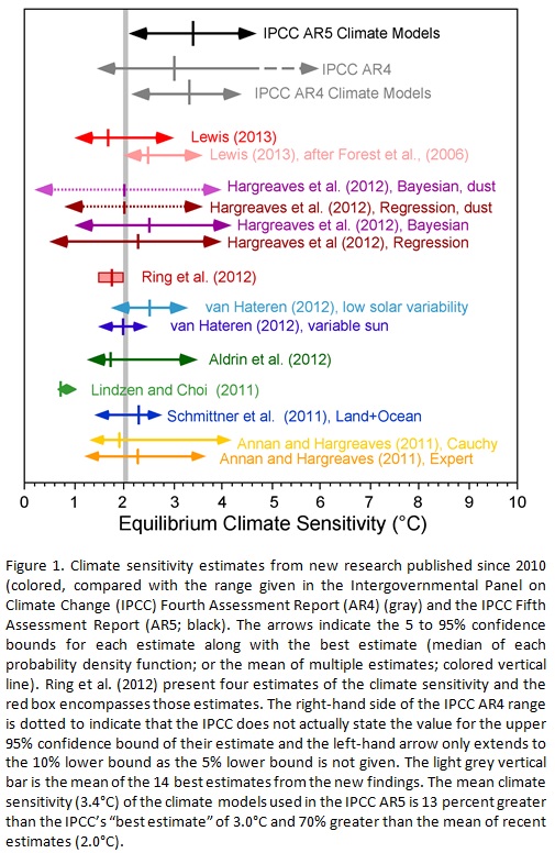
The determination of the global warming expected from a doubling of atmospheric carbon dioxide (CO2), called the climate sensitivity, is the most important parameter in climate science. The Intergovernmental Panel on Climate Change (IPCC) fifth assessment report (AR5) gives no best estimate for equilibrium climate sensitivity “because of a lack of agreement on values across assessed lines of evidence and studies.”
Studies published since 2010 indicates that equilibrium climate sensitivity is much less that the 3 °C estimated by the IPCC in its 4th assessment report. A chart here shows that the mean of the best estimates of 14 studies is 2 °C, but all except the lowest estimate implicitly assumes that the only climate forcings are those recognized by the IPCC. They assume the sun affects climate only by changes in the total solar irradiance (TSI). However, the IPCC AR5 Section7.4.6 says,
“Many studies have reported observations that link solar activity to particular aspects of the climate system. Various mechanisms have been proposed that could amplify relatively small variations in total solar irradiance, such as changes in stratospheric and tropospheric circulation induced by changes in the spectral solar irradiance or an effect of the flux of cosmic rays on clouds.”
Many studies have shown that the sun affects climate by some mechanism other than the direct effects of changing TSI, but it is not possible to directly quantify these indirect solar effects. All the studies of climate sensitivity that rely on estimates of climate forcings which exclude indirect solar forcings are invalid.
Fortunately, we can calculate climate sensitivity without an estimate of total forcings by directly measuring the changes to the greenhouse effect.
The greenhouse effect (GHE) is the difference in temperature between the earth’s surface and the effective radiating temperature of the earth at the top of the atmosphere as seen from space. This temperature difference is generally given as 33 °C, where the top-of-atmosphere global average temperature is about -18 °C and global average surface temperature is about 15 °C. We can estimate climate sensitivity by comparing the changes in the GHE to the changes in the CO2 concentrations.
The Clouds and Earth’s Radiant Energy System (CERES) experiment started collecting high quality top-of-atmosphere outgoing longwave radiation (OLR) data in March 2000. The last data available is June 2013 as of this writing on January 14, 2013. Figure 1 shows a typical CERES satellite.

Figure 1. CERES Satellite
The CERES OLR data presented by latitude versus time is shown in Figure 2.

Figure 2. CERES Outgoing Longwave Radiation, latitude versus date.
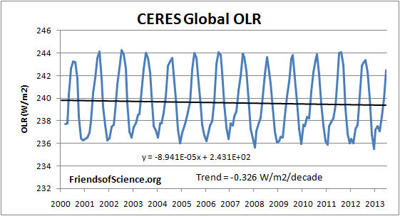
The global average OLR is shown in Figure 3.

Figure 3. CERES global OLR.
The CERES OLR data is converted to the effective radiating temperature (Te) using the Stefan-Boltzmann equation.
Te = (OLR/σ)0.25 – 273.15. where σ = 5.67 E-8 W/(m2K4), Te is in °C.
The monthly anomalies of the Te were calculated so that the annual cycle would not affect the trend.
We use the HadCRUT temperature anomaly indexes to represent the earth’s surface temperature (Ts). The HadCRUT3 temperature index shows a cooling trend of -0.002 °C/decade, and the HadCRUT4 temperature index shows a warming trend of 0.031 °C/decade during the period with CERES data, March 2000 to June 2013. The land measurement likely includes a warming bias due to uncorrected urban warming. The hadCRUT4 dataset added more coverage in the far north, where there has been the most warming, but failed to add coverage in the far south, where there has been recent cooling, thereby introducing a warming bias. We present results using both datasets.
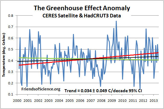
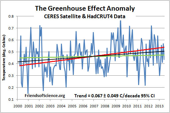
The difference between the surface temperatures anomaly and effective radiating temperature anomaly is the GHE anomaly. Figures 4 and 5 show the Greenhouse effect anomaly utilizing the HadCRUT3 and HadCRUT4 temperature indexes, respectively.

Figure 4. The greenhouse effect anomaly based on CERES OLR and HadCRUT3.

Figure 5. The greenhouse effect anomaly based on CERES OLR and HadCRUT4.
The trends of the GHE are 0.0343 °C/decade based on HadCRUT3, and 0.0672 °C/decade based on HadCRUT4.
We want to compare these trends in the GHE to changes in CO2 to determine the climate sensitivity. Only changes in anthropogenic greenhouse gases can cause a significant change in the greenhouse effect. Changes in the sun’s TSI, aerosols, ocean circulation changes and urban heating can’t change the GHE. Changes in cloudiness could change the GHE, but data from the International Satellite Cloud Climatology Project shows that the average total cloud cover during the period March 2000 to December 2009 changed very little. Therefore, we can assume that the measured change in the GHE is due to anthropogenic greenhouse gas emissions, which is dominated by CO2.
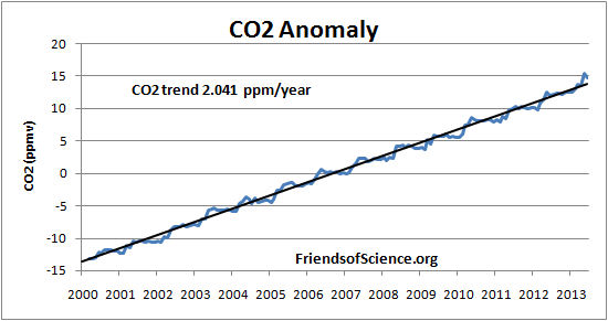
The CO2 data also has a large annual cycle, so the anomaly is used. Figure 6 shows the monthly CO2 anomaly calculated from the Mauna Loa data and the best fit straight line.

Figure 6. CO2 anomaly.
The March 2000 CO2 concentration is assumed to be the 13 month centered average CO2 concentration at March 2000, and the June 2013 value is that value plus the anomaly change from the fitted linear line. Table 1 below shows the CO2 concentrations, the logarithm of the CO2 concentration, and the change in the GHE from March 2000 for both the HadCRUT3 and HadCRUT4 cases.
Table 1 shows that the GHE has increased by 0.046 °C from March 2000 to June 2013 based on changes in the CERES OLR data and HadCRUT3 temperature data. Extrapolating to January 2100, the GHE increase to 0.28 °C by January 2100. Using the HadCRUT4 temperature data, the GHE increases by 0.55 °C by January 2100 compared to March 2000.
| hadCRUT3 | hadCRUT4 | |||
| Date | CO2 | Log CO2 | ΔGHE | ΔGHE |
| ppm | °C | °C | ||
| March 2000 | 368.88 | 2.567 | 0 | 0 |
| June 2013 | 395.94 | 2.598 | 0.046 | 0.089 |
| January 2100 | 572.68 | 2.758 | 0.283 | 0.554 |
| 2X CO2 | 737.76 | 2.868 | 0.446 | 0.873 |
Table 1. Extrapolated changes to the greenhouse effect (GHE) based on two versions of the hadCRUT datasets.
Table 1 shows that the GHE has increased by 0.046 °C from March 2000 to June 2013 based on changes in the CERES OLR data and HadCRUT3 temperature data. Extrapolating to January 2100, the GHE increase to 0.28 °C by January 2100. Using the HadCRUT4 temperature data, the GHE increases by 0.55 °C by January 2100 compared to March 2000.
The last row of Table 1 shows the transient climate response (TCR), which is the temperature response to CO2 emissions from March 2000 levels to the time when CO2 concentrations have doubled. TCR is less than the equilibrium climate sensitivity because the oceans have not reached temperature equilibrium at the time of CO2 doubling. TCR is calculated by the equation:
TCR = F2x dT/dF ; where dT means the temperature difference, dF means the forcing difference, from March 2000 to June 2013.
The CO2 forcing was calculated as 5.35 x ln (CO2/CO2i). The change in forcing from March 2000 to June 2013 is 0.379 W/m2. The forcing for double CO2 (F2x) is 3.708 W/m2. The TCR is 0.45 °C using hadCRUT3, and 0.87 °C using hadCRTU4 data. These values are much less than the multi-model mean estimate of 1.8 °C for TCR given in Table 9.5 of the AR5. The climate model results do not agree with the satellite and surface data and should not be used to set public policies.
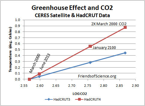
Figure 7 shows the results of Table 1 graphically.

Figure 7. The greenhouse effect and CO2 extrapolated to January 2100 and double CO2 bases on CERES and HadCRUT data.
This analysis suggests that the temperature change from June 2013 to January 2100 due to increasing CO2 would be 0.24 °C (from HadCRUT3) or 0.46 °C (from HadCRUT4), assuming the CO2 continues to increase along the recent linear trend.
An Excel spreadsheet with the data, calculations and graphs is here.
HadCRUT3 data is here.
HadCRUT4 data is here.
Mauna Loa CO2 data is here.
CERES OLR data is here.
Total cloud cover data is here.
Bill Marsh says: January 16, 2014 at 5:29 am
It implies that natural sources of CO2, averaged over the annual cycle, does not change other than any feedback temperature response. There is an obvious annual cycle of natural CO2 production and absorption. I used the CO2 anomaly to calculate the CO2 trend so the annual cycle doesn’t affect the trend. There was no temperature change during the CERES period, so there was no feedback response of natural CO2 production. If volcanoes increased emissions, sure, that would affect the trend, but there have been no major volcanic eruption during the period, and volcanic CO2 is very small compared to human sources.
Ken
A change of TSI it would change both the surface temperature (Ts) and the effective radiating temperature (Te) equally
Don’t think so. Ts would rise faster than Te, even with constant GHE.
Norm Kalmanovitch says: January 16, 2014 at 5:18 am
Hmmm says: January 16, 2014 at 5:36 am
My calculations are based on changes in the GHE. How do the think PDO and AMO affects longwave absorption, downward longwave radiation, or the Ts-Te difference? They can’t. PDO and AMO affects surface temperatures Ts, but do not change the GHE.
MikeB says: “I believe Brian Cox performed such a TV experiment by warming a pan of water under full sun and estimating the watts required for such heating.”
You are correct he did such a experiment in Death Valley I believe and demonstrated that some 1000 W/m^2 was raining down on the earth at that location. Tough to get 255 K out of 1000 W/m^2.
Not on subject but: Per the EIA (Energy Info Agency) the 2nd week of Jan. Natural Gas net draw from storage was 287 Billion cu. ft. This is a record draw for any week of the heating season for the past 21 seasons. The second highest record 285 B cu ft was the second week of Dec 2013 also this season. The previous record draw was 266 billion cu ft the 2nd week of Jan 2010. Any time the draw exceeds 200 B Cu Ft It usually correlates with a negative temperature anomaly in the US for that week.
The following link provides access to a XL storage history spread sheet link.
http://ir.eia.gov/ngs/ngs.html
richardscourtney says: January 16, 2014 at 5:44 am
Richard, I agree with everything you said here, and for a technical journal submission, a statistical analysis with 95% confidence intervals would be necessary. A 95% confidence range of possible values for TCR would be significantly wider than the two values I presented. The uncertainties are much more than just the random noise. We don’t know what systematic errors are in the surface and satellite measurements, so even a 95% confidence interval will not give the full range of possible values. It is clear that the values presented are just the best estimates based on the two datasets used. That is fine for a blog post.
Eric Worrall says:
January 16, 2014 at 1:46 am
Purely gravitational lapse rates are refuted by this essay. If the lapse rate were due to gravity, it would be possible to create a perpetual motion machine powered by said gravity.
http://wattsupwiththat.com/2012/01/24/refutation-of-stable-thermal-equilibrium-lapse-rates/
====================================================================
The problem with the supposed proof is that it uses an unmodified version of Fourier’s Law. If there is an exchange of kinetic and gravitational potential energy in the gas column, then there must also be a similar exchange that goes on in the silver wire.
I really don’t understand all the resistance to this idea. It’s as if proof of the existence of atoms is still in doubt.
If one believes in atoms, then one must accept that as they move through a gravitational field that there will be an exchange of kinetic energy and gravitational potential energy. Collisions don’t change this.
Joe Born says: January 16, 2014 at 7:29 am
Willis Eschenbach had commented on this point a few times. The 4th root of the average surface radiation flux is not quite equal to the average of the 4th root of the surface radiation fluxes. Over the range of temperatures we are dealing with, the error is small. I don’t think this is relevant to my post because the the earth’s temperature range over the surface area has not likely changed over the 13 year period, so it wouldn’t affect the trends.
The surface of the Earth with no atmosphere would be the same as the moon, which is at 127 deg C in sunlight (-173 deg C on the dark side).
As climate models assume 24 hour a day sunlight, the 127 deg C temperature is applicable.
So, without an atmosphere, the Earth would be at 127 deg C at the surface and, instead, with an atmosphere is at 15 deg C. It is not a big stretch to see that the atmosphere clearly cools the planet’s surface, giving the surface more ways to shed heat, by conduction and convection, rather than just by radiation with no atmosphere.
As the temperature of the upper atmosphere varies with altitude quite radically, it makes no sense to pretend that there is a greenhouse effect that does not resemble a greenhouse at all and whose conditions are essentially arbitrarily chosen.
It doesn’t add up… says:
January 16, 2014 at 7:11 am
The moon has a Bond albedo of 0.11, and a SB theoretical temperature of 270.7K according to NASA:
http://nssdc.gsfc.nasa.gov/planetary/factsheet/moonfact.html
Yet the average temperature at the equator (the hottest latitude) is just 206K according to NASA using its Diviner measurements:
http://diviner.ucla.edu/science.shtml
There is no significant atmosphere, but a large divergence between supposed theory and actual measurement.
The lunar surface absorbs some energy and re-emits it, but it also reflects some without absorption. Presumably then the surface heating is less than total incoming energy. Presumably at least some of the difference can be accounted for by that.
“Changes in the sun’s TSI, aerosols, ocean circulation changes and urban heating can’t change the GHE.”
But increased NPP can account for at least a portion of reduced outgoing LWR.
What,for goodness sake is going on here !. Barely four days after this site invited a guest to write an article that included this –
‘GLOBAL WARMING IS REAL’
“Yes, the world has warmed 1°F to 1.5°F (0.6°C to 0.8°C) since 1880 when relatively good thermometers became available. Yes, part of that warming is due to human activities, mainly burning unprecedented quantities of fossil fuels that continue to drive an increase in carbon dioxide (CO2) levels. The Atmospheric “Greenhouse” Effect is a scientific fact!”
Damnest thing I have seen in over two decades on the forums
‘Any chance of an essay expanding on and consolidating all @AlecM’s points? That would be really useful!”
Yes, submit them to the nobel prize committee. Were he correct he would surely win the prize.
It bears repeating
‘Roy Spencer says:
January 16, 2014 at 2:10 am
you cannot estimate radiative feedbacks (climate sensitivity) without knowing the radiative forcing(s), both natural and manmade. Forcings and feedbacks are intermingled in unknown proportions, and CERES measures the sum of both.”
“higley7 says:
January 16, 2014 at 9:51 am
The surface of the Earth with no atmosphere would be the same as thhe moon, which is at 127 deg C in sunlight (-173 deg C on the dark side).
As climate models assume 24 hour a day sunlight, the 127 deg C temperature is applicable.”
######################
WRONG. yes virginia climate models have day and night. That is how, for example, we compare the diurnal range between models and observations.
knowledge is limited but stupidity is unbounded
Eric Worrall:”Purely gravitational lapse rates are refuted by this essay. If the lapse rate were due to gravity, it would be possible to create a perpetual motion machine powered by said gravity.”
Scot: “The problem with the supposed proof is that it uses an unmodified version of Fourier’s Law. If there is an exchange of kinetic and gravitational potential energy in the gas column, then there must also be a similar exchange that goes on in the silver wire.”
For the reasons I gave on that thread, I agree that Dr. Brown’s “refutation” left something to be desired. But, although as I read them the papers cited on that thread dictate an equilibrium kinetic-energy gradient, the gradient they specify is as a practical matter too small to be measured. Indeed, it may be too small to be measured even in principle. For all practical purposes, that is, the temperature in a gravitational field would be uniform at equilibrium.
But differential surface heating and conduction from the surface to the atmosphere would still happen even if the atmosphere were perfectly transparent, so equilibrium still wouldn’t prevail. Whether the resultant disturbances would result in much of a lapse rate is another question, though.
Joe Born says: January 16, 2014 at 8:17 am
Climate sensitivity to CO2 is the ratio of the surface temperature change that was caused by CO2 increases, including any feedbacks, to the change in CO2 forcing that caused that temperature change. But we don’t know directly what part of the surface temperature change was caused by the CO2 change. The greenhouse effect is the difference between the surface temperatures and the top-of-atmosphere temperatures, determined by OLR. OLR can change over the short term for many reasons not related to CO2. But the GHE changes primarily by changes in greenhouse gases, which affect the longwave radiation, not shortwave. Changes is albedo from changes in “cloud and snow reflection of short-wave radiation” will change surface temperatures and will change OLR, but will not change the GHE, which depends on longwave absorption and the resulting back radiation. That is, albedo changes Ts and Te equally, so no change in Ts – Te = GHE. So no, we don’t need to know the changes in short-wave radiation to calculate climate sensitivity.
AlecM 3:17am: “The Law of Conservation of Energy between the material and EM worlds is: qdot = -Div Fv where qdot is the monochromatic rate of heat generation per unit volume of matter and Fv is the monochromatic radiative flux density…I …made real measurements “
Cite? I am interested to read up on your publications or those of others that are similar, thx. The top post discussion of forcings, GHE and atm. fluid SW/OLR energy conservation seems complete enough without need of applying this formula.
One of the few others you claim exist “..around the World set out to understand the real nature of radiative energy transfer” published Radiative Heat Transfer 3rd. ed. 2013 – Dr. Michael F. Modest. So I pulled out a copy to try and understand your clipped equation. (Wish he had called it Radiative Energy Transfer but that’s just a SIF for you).
Here the text book shows qdot term is as you imply “..the heat generated within the medium (such as energy release due to chemical reactions).” p.297. Since the medium is earth’s atm. this qdot term must be 0 as the atm. uses up no reservoir on its own generating energy, the atm. energy is ultimately derived from using up sun’s H reservoir.
To obtain your steady state simplification for atm. radiative equilibrium the qdot = 0 = -Div Fv (eqn. 10.75 which is just 0 = SW energy in – LW energy out, i.e. for a planet LTE) from the general form of the energy conservation equation (10.70) for a moving compressible fluid; Dr. Modest explains the situation must be where radiation is the dominant mode of heat transfer, meaning that convection and conduction are negligible. Radiative equilibrium using this formula you write is applicable extremely high temperatures, plasmas, nuclear reactions that happen fast* where conduction and convection are negligible and so forth p. 298 – quite unlike the atm.
Lord Kelvin in 1862 wrote a paper that still stands today showing convection is the dominant mode of energy transfer in Earth’s atmosphere (cite Bohren 1998 for discussion).
I am curious how you can apply and draw correct conclusions from this formula on earth atm. based on making “real measurements of coupled convection and radiation”. I would like to understand why you claim “It’s a Big Mess and until Climate Alchemy dumps the ‘back radiation’ and ‘forcing’ concepts, there can be no progress…”
NB: *fast = being defined as the cases where radiative transfer occurs so fast that radiative equilibrium is achieved before a noticeable change in temperature occurs (so can drop the unsteady terms in generalized fluid energy cons.).
@ur momisugly Duster:
That’s the point: do the sum T= ((1-A)1367.5/4s)^0.25 where s= SB constant or 5.67 e-8; and A is 0.11 – the Bond Albedo and the factor 4 comes from the ratio between the cross section area and surface area of a sphere, and you’ll get 270.7 K – which takes account of the reflected energy via the albedo, and is the “grey body” temperature. Peak temperatures measured by Diviner are higher than the 383K implied by overhead sunshine at an albedo of 0.11, but the albedo is of course not constant across the surface.
Measure the actual temperatures, and they come out lower on average, even along the equator, where they ought to be higher than the average for the whole moon (the polar temperatures are much lower, because of the shallow angle of insolation – see the chart of temperature by latitude at the Diviner link I gave).
So if the model doesn’t work for a body with no atmosphere, it won’t work for one which has one.
lgl says: January 16, 2014 at 8:49 am
Wikipedia might not be the best source, but it is easy. The “Greenhouse effect” article says,
So yes, GHE = Ts -Te. Therefore, if GHE is constant, a change in surface temperature would be matched by the same change in the effective radiating temperature.
Note the Wikipedia author can’t add! 14 C – (-18 C) = 32 C, not 33 C. The surface temperature should be about15 C.
Why do the think Ts would rise faster than Te?
Ken Gregory:
Thankyou for taking the trouble to again answer me as you do in your post at January 16, 2014 at 9:22 am. Your answer quotes from my second post then replies saying in total.
I ask you to understand that I like your article and my comments are because I like it I am trying to provide constructive criticism (n.b. I am NOT carping), and I am doing this because I do not want inadequacies to be used as reason to refute and/or denigrate your work.
I am pleased that I managed to adequately state my point at my second attempt and that we are in complete agreement about it.
I agree all that you say in your reply (which I here quote) except for your final sentence.
Importantly, I strongly agree with you that the systematic errors are not known and this does require mention. However, I said the inherent errors of the data should be considered and concluded from that saying at the end of my first post
and you now agree that saying
But you then add your final sentence which says
It is my disagreement with that which has induced my comments to you.
Anybody can say (and such as SkS will say), “Gregory’s analysis is wrong because it ignores the variance of the data. It is only a blog post that is not good enough to publish in a journal”.
But I think Gregory’s analysis is right and if it took account of inherent errors in the data then it could be published in a journal.
Richard
Gkell1:
At January 16, 2014 at 10:11 am you ask
Allow me to answer your query.
The atmospheric Greenhouse Effect (GE) is an accepted scientific theory.
But man-made global warming (i.e. anthropogenic Global Warming or AGW) resulting from enhancement of the GE by human activities is merely a conjecture.
Sadly, some people think the GE is AGW but the GE has existed since long before humans.
In the thread you mention I wrote this.
The above analysis attempts to provide information to determine if it is possible for AGW to become sufficiently large for AGW to be discernible. That is good information to obtain if you think AGW can become a problem or if you think it cannot.
Richard
@Trick: the equation comes from Goody and Yung, Atmospheric Physics, Oxford Academic Press and, as i stat4d, simply the Law of Conservation of Energy but between matter (kinetic) and EM energy.
You integrate this over time, space and wavelengths to get the difference between two S-B equations, which give the Radiation Fields at the start and the finish of the element of matter. Net EM energy flux converted to kinetic energy = -integral(delta RF dt)
The negative sign is missed by those who confuse kinetic and EM energy, most scientists and engineers from my experience, and it took me (and Claes Johnson perhaps?) some time to correct my own misconceptions.
I just hope that Climate Alchemists like Trenberth soon stop the ludicrous ‘back radiation’ and forcing concepts.
mkelly says:
January 16, 2014 at 9:02 am
1000 W/m^2. seems about right when the sun directly overhead in a clear sky. The sun probably never gets directly overhead in Death Valley, but close. What you have to take into account is that when the sun is overhead in one place, it is not overhead over the rest of the earth. It provides no heat input at all to the darkside for example. Averaged over the surface area of the earth we get a solar input at the surface of about 240 W/m^2. Now, according to the Stephan-Boltzmann Law, 240 W/m^2 is equivalent to a temperature of 255K. That’s how we get it. Not too tough I hope?