Guest essay by Ken Gregory
See abstract and PDF version here.
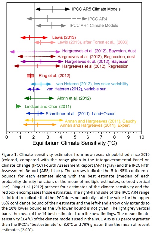
The determination of the global warming expected from a doubling of atmospheric carbon dioxide (CO2), called the climate sensitivity, is the most important parameter in climate science. The Intergovernmental Panel on Climate Change (IPCC) fifth assessment report (AR5) gives no best estimate for equilibrium climate sensitivity “because of a lack of agreement on values across assessed lines of evidence and studies.”
Studies published since 2010 indicates that equilibrium climate sensitivity is much less that the 3 °C estimated by the IPCC in its 4th assessment report. A chart here shows that the mean of the best estimates of 14 studies is 2 °C, but all except the lowest estimate implicitly assumes that the only climate forcings are those recognized by the IPCC. They assume the sun affects climate only by changes in the total solar irradiance (TSI). However, the IPCC AR5 Section7.4.6 says,
“Many studies have reported observations that link solar activity to particular aspects of the climate system. Various mechanisms have been proposed that could amplify relatively small variations in total solar irradiance, such as changes in stratospheric and tropospheric circulation induced by changes in the spectral solar irradiance or an effect of the flux of cosmic rays on clouds.”
Many studies have shown that the sun affects climate by some mechanism other than the direct effects of changing TSI, but it is not possible to directly quantify these indirect solar effects. All the studies of climate sensitivity that rely on estimates of climate forcings which exclude indirect solar forcings are invalid.
Fortunately, we can calculate climate sensitivity without an estimate of total forcings by directly measuring the changes to the greenhouse effect.
The greenhouse effect (GHE) is the difference in temperature between the earth’s surface and the effective radiating temperature of the earth at the top of the atmosphere as seen from space. This temperature difference is generally given as 33 °C, where the top-of-atmosphere global average temperature is about -18 °C and global average surface temperature is about 15 °C. We can estimate climate sensitivity by comparing the changes in the GHE to the changes in the CO2 concentrations.
The Clouds and Earth’s Radiant Energy System (CERES) experiment started collecting high quality top-of-atmosphere outgoing longwave radiation (OLR) data in March 2000. The last data available is June 2013 as of this writing on January 14, 2013. Figure 1 shows a typical CERES satellite.

Figure 1. CERES Satellite
The CERES OLR data presented by latitude versus time is shown in Figure 2.

Figure 2. CERES Outgoing Longwave Radiation, latitude versus date.
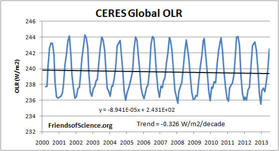
The global average OLR is shown in Figure 3.

Figure 3. CERES global OLR.
The CERES OLR data is converted to the effective radiating temperature (Te) using the Stefan-Boltzmann equation.
Te = (OLR/σ)0.25 – 273.15. where σ = 5.67 E-8 W/(m2K4), Te is in °C.
The monthly anomalies of the Te were calculated so that the annual cycle would not affect the trend.
We use the HadCRUT temperature anomaly indexes to represent the earth’s surface temperature (Ts). The HadCRUT3 temperature index shows a cooling trend of -0.002 °C/decade, and the HadCRUT4 temperature index shows a warming trend of 0.031 °C/decade during the period with CERES data, March 2000 to June 2013. The land measurement likely includes a warming bias due to uncorrected urban warming. The hadCRUT4 dataset added more coverage in the far north, where there has been the most warming, but failed to add coverage in the far south, where there has been recent cooling, thereby introducing a warming bias. We present results using both datasets.
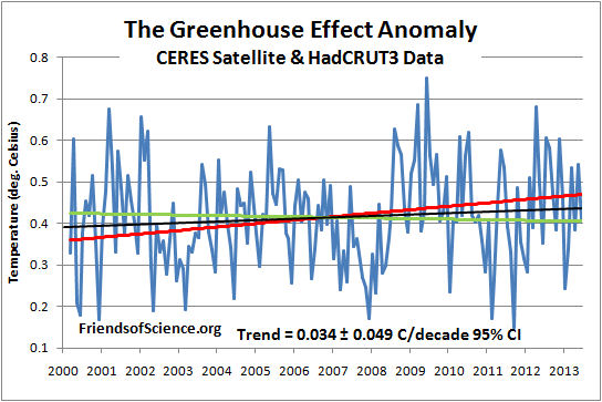
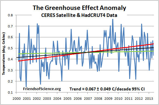
The difference between the surface temperatures anomaly and effective radiating temperature anomaly is the GHE anomaly. Figures 4 and 5 show the Greenhouse effect anomaly utilizing the HadCRUT3 and HadCRUT4 temperature indexes, respectively.

Figure 4. The greenhouse effect anomaly based on CERES OLR and HadCRUT3.

Figure 5. The greenhouse effect anomaly based on CERES OLR and HadCRUT4.
The trends of the GHE are 0.0343 °C/decade based on HadCRUT3, and 0.0672 °C/decade based on HadCRUT4.
We want to compare these trends in the GHE to changes in CO2 to determine the climate sensitivity. Only changes in anthropogenic greenhouse gases can cause a significant change in the greenhouse effect. Changes in the sun’s TSI, aerosols, ocean circulation changes and urban heating can’t change the GHE. Changes in cloudiness could change the GHE, but data from the International Satellite Cloud Climatology Project shows that the average total cloud cover during the period March 2000 to December 2009 changed very little. Therefore, we can assume that the measured change in the GHE is due to anthropogenic greenhouse gas emissions, which is dominated by CO2.
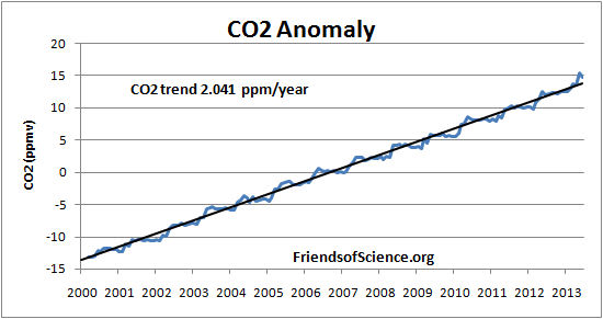
The CO2 data also has a large annual cycle, so the anomaly is used. Figure 6 shows the monthly CO2 anomaly calculated from the Mauna Loa data and the best fit straight line.

Figure 6. CO2 anomaly.
The March 2000 CO2 concentration is assumed to be the 13 month centered average CO2 concentration at March 2000, and the June 2013 value is that value plus the anomaly change from the fitted linear line. Table 1 below shows the CO2 concentrations, the logarithm of the CO2 concentration, and the change in the GHE from March 2000 for both the HadCRUT3 and HadCRUT4 cases.
Table 1 shows that the GHE has increased by 0.046 °C from March 2000 to June 2013 based on changes in the CERES OLR data and HadCRUT3 temperature data. Extrapolating to January 2100, the GHE increase to 0.28 °C by January 2100. Using the HadCRUT4 temperature data, the GHE increases by 0.55 °C by January 2100 compared to March 2000.
| hadCRUT3 | hadCRUT4 | |||
| Date | CO2 | Log CO2 | ΔGHE | ΔGHE |
| ppm | °C | °C | ||
| March 2000 | 368.88 | 2.567 | 0 | 0 |
| June 2013 | 395.94 | 2.598 | 0.046 | 0.089 |
| January 2100 | 572.68 | 2.758 | 0.283 | 0.554 |
| 2X CO2 | 737.76 | 2.868 | 0.446 | 0.873 |
Table 1. Extrapolated changes to the greenhouse effect (GHE) based on two versions of the hadCRUT datasets.
Table 1 shows that the GHE has increased by 0.046 °C from March 2000 to June 2013 based on changes in the CERES OLR data and HadCRUT3 temperature data. Extrapolating to January 2100, the GHE increase to 0.28 °C by January 2100. Using the HadCRUT4 temperature data, the GHE increases by 0.55 °C by January 2100 compared to March 2000.
The last row of Table 1 shows the transient climate response (TCR), which is the temperature response to CO2 emissions from March 2000 levels to the time when CO2 concentrations have doubled. TCR is less than the equilibrium climate sensitivity because the oceans have not reached temperature equilibrium at the time of CO2 doubling. TCR is calculated by the equation:
TCR = F2x dT/dF ; where dT means the temperature difference, dF means the forcing difference, from March 2000 to June 2013.
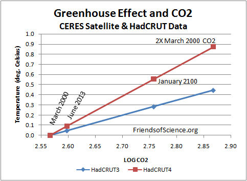
The CO2 forcing was calculated as 5.35 x ln (CO2/CO2i). The change in forcing from March 2000 to June 2013 is 0.379 W/m2. The forcing for double CO2 (F2x) is 3.708 W/m2. The TCR is 0.45 °C using hadCRUT3, and 0.87 °C using hadCRTU4 data. These values are much less than the multi-model mean estimate of 1.8 °C for TCR given in Table 9.5 of the AR5. The climate model results do not agree with the satellite and surface data and should not be used to set public policies.
Figure 7 shows the results of Table 1 graphically.

Figure 7. The greenhouse effect and CO2 extrapolated to January 2100 and double CO2 bases on CERES and HadCRUT data.
This analysis suggests that the temperature change from June 2013 to January 2100 due to increasing CO2 would be 0.24 °C (from HadCRUT3) or 0.46 °C (from HadCRUT4), assuming the CO2 continues to increase along the recent linear trend.
An Excel spreadsheet with the data, calculations and graphs is here.
HadCRUT3 data is here.
HadCRUT4 data is here.
Mauna Loa CO2 data is here.
CERES OLR data is here.
Total cloud cover data is here.
@steveta_uk: “Why does AlexM repeat the same claims on every thread that mentions the GHE despite being unable to convince anyone ever that he knows what he’s talking about?”
Answer: because until somebody comes up with a scientific argument, backed up by experimental evidence, proving that I am wrong, it is my duty as a scientist to push the bloody point ad nauseum.
No-one has yet taken me on, probably because I am one of the very few still active who has made real measurements of coupled convection and radiation, and have along with very few others around the World set out to understand the real nature of radiative energy transfer.
I’ll give you an example. The Law of Conservation of Energy between the material and EM worlds is: qdot = -Div Fv where qdot is the monochromatic rate of heat generation per unit volume of matter and Fv is the monochromatic radiative flux density. All scientists and engineers i have talked to forget about the negative sign. Many otherwise competent physicists imagine matter fires out photons according to the S-B equation. This explains why Sagan and Houghton got it wrong.
It’s a Big Mess and until Climate Alchemy dumps the ‘back radiation’ and ‘forcing’ concepts, there can be no progress except phoney modelling to pretend the subject knows what it is doing. That does’t fool me and Nature is showing the reality, which is that the claimed CO2 climate sensitivity of the IPCC is a lavishly-funded confidence trick.
I hate and loath all use of ‘Linear Trends’, OLS or otherwise. They are only of use to infill values within the period they cover (at best). They are completely useless outside of the data range they are drawn from.
‘Linear Trends’ = ‘Tangent to the curve’ = ‘Flat Earthers’.
“‘Linear Trends’ = ‘Tangent to the curve’ = ‘Flat Earthers’.”
– – –
When you watch a movie or play a game console game that uses computer generated graphics, every pixel for the image is generated from straight lines. This also applies to Finite Element Analysis for engineering applications. Its really a matter of computer resources that determines the accuracy.
richardscourtney says: January 16, 2014 at 2:34 am
The temperature trend is near zero, but the trend in the greenhouse effect is significantly positive. You can judge the uncertainties in the estimates by observing how closely the greenhouse effect curves follow the best fit line. The R2 value for the fit in Figure 4 for HadCrut3 is R2 = 0.012. The difference in the TCR results between HadCRUT3 and HadCRUT4, 0.45 C and 0.87 C, respectively, further shows that the TCR is uncertain. The data is messy, that that is the best we have.
This calculation does not require direct knowledge of the total forcings operating in the climate system. The forcing from indirect solar effects are unknown, but they must be substantial because there are strong correlations between solar activity and global temperatures. Any method to estimate climate sensitivity that requires an estimate of total forcing but only uses the IPCC recognized forcings are totally useless because they ignore indirect solar forcings.
You provided a link to my article “Out-going Longwave Radiation and the Greenhouse Effect” which estimates climate sensitivity at 0.4 C. That paper used a long dataset from 1960, and used radiosonde humidity data to calculate OLR, which is uncertain, but the general method is the same. This article uses a short, but high quality CERES dataset, and also gets low climate sensitivity.
@ur momisugly RichardLH , Upon a second reading of your statement, “They are completely useless outside of the data range they are drawn from” is something I agree with somewhat. A trend line is different than a trend but unfortunately the general public are not versed in these nuances, as I was not 4 years ago either. (Thanks WUWT and W. M. Briggs amongst others for the education).
The blackbody radiation equates to a surface temperature of -18 degrees.
Why should we assume that the “surface” as seen by an instrument in space is ground level and not some altitude within our atmosphere? How is the lapse rate accommodated by GHG theory or is it ignored?
AlecM said:
“Answer: because until somebody comes up with a scientific argument, backed up by experimental evidence, proving that I am wrong, it is my duty as a scientist to push the bloody point ad nauseum.”
That’s how I feel, too 🙂
We still have people saying no lapse rate without GHGs when there obviously would be a lapse rate due to decreasing density with height and uneven surface heating leading to density variations with lighter air parcels rising above heavier parcels which is all that convection is.
garymount says:
January 16, 2014 at 3:56 am
It is just a nice ‘trick’ to be able to use the ‘flat earthers’ gibe in reverse sometimes, usually against CAGW.
‘Linear trends’ are not trends, they are lines drawn on a range of data, useless outside of the data range they are drawn on.
An elegant analysis.
In 2007 Stephen Schwartz of the Brookhaven Lab did a study base on ocean heat content and came up with 1.1 ± 0.5 K. Heat capacity, time constant, and sensitivity of Earth’s climate system. Schwartz S. E. J. Geophys. Res., 112, D24S05 (2007). doi:10.1029/2007JD008746
Given Schwartz’s wide error bars his lower would be 0.6 and upper 1.7 K.
The average of your figures of 0.45 °C and 0.87 °C is,0.66 K and that figure is within the range estimated by Schwartz..
Since the two methodologies are completely unconnected this is an impressive effort on your part. Why not publish?.
AlecM says:
January 16, 2014 at 3:17 am
Right on Alec.
You do not have to convince me.
@steveta_uk ; you are going to have do your homework before making untrue comments.
He should also read this post………
“johnmarshall says:
January 16, 2014 at 2:54 am ”
@steveta_uk ; try this:
http://greenhouse.geologist-1011.net/
1) If the CO2 increase is largely anthropogenic as claimed by the IPCC, why does Figure 6 show no evidence of the decrease in consumption in much of the world after the 2008 financial crisis?
Global CO2 emission in Gt/a (BP Statistical Review 2013)
2004….28.603
2005….29.453
2006….30.320
2007….31.197
2008….31.540
2009….31.100
2010….32.840
2011….33.743
2012….34.466
The change is not large enough to show clearly in the atmospheric total CO2 – especially when there are other sources and sinks to be accounted for.
A trend is a trend is a trend
But the question is, will it bend?
Will it alter its course
Through some unforeseen force
And come to a premature end?
Sir Alec Cairncross, economist.
Schrodinger’s Cat says:
January 16, 2014 at 4:02 am
We don’t assume that. We are able to determine the temperature of planets and stars by observing the spectrum of radiation that they produce. This has been possible for over 100 years.
Seen from space, we would assess the temperature of the earth to be 255K. Even before the satellite era, it was possible to make some assessment by estimating the solar radiation reaching the earth, on the basis that of what comes in equals what goes out (conservation of energy). I believe Brian Cox performed such a TV experiment by warming a pan of water under full sun and estimating the watts required for such heating.
So, in summary, we see the temperature of the earth from space as being 255K, but we know by living here that the SURFACE of the earth is much hotter than that. So how is the discrepancy explained? That is where the GHE comes in, and it is excellently explained in an earlier WUWT post this month http://wattsupwiththat.com/2014/01/12/global-warming-is-real-but-not-a-big-deal-2/
Even before Arrihenius’s paper of 1896 it was realised that “the temperature of the earth would probably fall to -200 degC if the atmosphere did not possess the quality of selective absorption” (a figure we now know to be much too low).
The greenhouse effect was a topic of study in our 1970 theoretical geophysics course. At that time the greenhouse effect was a theoretical metric for comparing the atmospheric insulation of the planets. we did this using the solar constant of 1367W/m^2 (and an appropriate increase for Venus which is closer and for Mars which is further). We used 0.3 for the Earth’s albedo and assumed a surface temperature of 288 k (approximately 15°C). This gave us 255 k for the effective radiative temperature which subtracted from the 288 k surface temperature gave us 33°C for the greenhouse effect.
Ken’s calculation of the greenhouse effect based on CERES OLR data covers the period since 2000 during which there was net global cooling. This exposes the fallacy of AGW in two ways.
First of all the CERES OLR data shows a net decrease in OLR with cooling temperatures. For this to occur there has to be a net decrease in incoming energy and since this change is not visible in the TSI measurement the only source for this decrease in incoming energy is increased albedo from a net increase in cloud cover.
The second and more critical aspect to the issue of AGW is that the greenhouse effect is increasing as the temperature is decreasing which is contrary to the AGW conjecture which would require a decrease in greenhouse effect with decreasing temperature for the AGW hypothesis to be valid and this is simply not the case.
Since the issue here is global warming and there has been a net 0.4°C of global warming since 1980 (ending by 1997), to see how this relates to global warming we need to look at OLR data covering the period when warming occurred. Fortunately this data was recorded by weather satellites since their launch in late 1978 and a graph of this OLR data is nicely presented on the Climate for You website (www.climate4you.com) compiled from data available from NOAA at http://www.esrl.noaa.gov/psd/data/gridded/data.interp_OLR.html
This dataset is clearly not as accurate as the CERES data showing OLR to be on average 232W/m^2 compared to the 239W/m^2 shown on the CERES data, but it does go back to when the global temperature was increasing and can provide the basis for a calculation of the greenhouse effect over the period from 1980 to 2010.
When calculated for these two years the greenhouse effect actually decreased from 35.56°C in 1980 to 35.42°C in 2010 demonstrating that the 70.9% increase in CO2 emissions since 1980 never actually enhanced the greenhouse effect and therefore completely refuting the basis for AGW conjecture.
Ken’s demonstration using CERES OLR data shows an increase in greenhouse effect with decreasing global temperature and my demonstration using OLR data from weather satellites shows decreasing greenhouse effect with increasing global temperature. Either of these demonstrations proves that changes to incoming energy from changes in albedo and definitely not CO2 is driving the changes in global temperature and combined these demonstrations make the proof incontrovertible. This change in albedo is demonstrated by Project Earthshine which shows the albedo decreasing to 1998 and then increasing since.
A change in albedo resulting from changes in cloud cover fits very nicely with Svensmark’s hypothesis of solar activity controlled cosmic ray cloud nucleation giving us both confirmation of solar theory for global temperature change and incontrovertible evidence that the AGW hypothesis is pure bunk.
“Only changes in anthropogenic greenhouse gases can cause a significant change in the greenhouse effect. ”
I don’t understand why you believe this base assumption to be axiomatic. Doesn’t it imply that all natural sources of CO2 are constant?
I think you could only do this if you had data extending beyond known cycles (60-80 years to cover a complete PDO, AMO etc…). Because of where we are in the PDO cycle with this data, I would have to assume your result estimates the lower bound rather than the center.
Ken Gregory:
Thankyou for your post at January 16, 2014 at 3:44 am
http://wattsupwiththat.com/2014/01/16/ceres-satellite-data-and-climate-sensitivity/#comment-1537703
in reply to my post at January 16, 2014 at 2:34 am
http://wattsupwiththat.com/2014/01/16/ceres-satellite-data-and-climate-sensitivity/#comment-1537664
Obviously, I was not clear because your reply does not answer my point. I will try to do better this time.
I wrote
I bolded that to ensure it would not be missed so it must be that it is not sufficiently clear.
Your results are obtained from the AVERAGE trend of each time series you analysed. But the data are noisy and – as you agree – the average trend is near zero in each case. Indeed, as I said, the difference between the trends of the two data sets spans zero.
Your obtained range of results is not valid because you have adopted unjustifiable trend values.
For example, you could have used zero trend and obtained a single and different result. But you used the average trend of each data set to provide a single result from each of the two data sets then quoted the obtained results to provide a range; i.e. between 0.24 °C to 0.46 °C for projected indicated global temperature rise projections to January 2100.
Each data set provides a range of possible trend values to within specified confidence (climate science uses 95% confidence). Hence, there is a maximum trend and a minimum trend at 95% confidence for EACH of your two analysed time series. Using these values would provide A RANGE OF PROJECTIONS FOR EACH DATA SET to within 95% confidence.
A combination of the two analyses would then obtain a wide range from the lowest of the two minimum projections to the highest of the two maximum projections and would be to 95% confidence.
In conclusion, using the average trend of each data set provides results which are induced by the variances of the data sets. In other words, your results are solely a result of ‘noise’ in the data. But, as I have explained, you could re-do the analysis to provide valid results with stated confidence.
Richard
The moon has a Bond albedo of 0.11, and a SB theoretical temperature of 270.7K according to NASA:
http://nssdc.gsfc.nasa.gov/planetary/factsheet/moonfact.html
Yet the average temperature at the equator (the hottest latitude) is just 206K according to NASA using its Diviner measurements:
http://diviner.ucla.edu/science.shtml
There is no significant atmosphere, but a large divergence between supposed theory and actual measurement.
Eric Worrall says:
January 16, 2014 at 1:46 am
Purely gravitational lapse rates are refuted by this essay.
http://wattsupwiththat.com/2012/01/24/refutation-of-stable-thermal-equilibrium-lapse-rates/
==========
I reread Dr Brown’s essay. From what I read he is not attributing the lapse rate to GHG. Rather to rising and falling parcels of air due to heating and cooling of the surface. These rising and falling parcels of air would still exist in the absence of GHG due to the rotation of the earth and seasonal differences, thus the lapse rate cannot be a product of GHG.
This is further confirmed by the dry air lapse rate 9.8C/km being equivalent to gravitational acceleration 9.8 m/s2.
It seems clear that the DALR is a result of conversion of PE to/from KE, and the energy to drive the system comes primarily from heating of the surface, either by the sun or the earth’s core. Without this heating the atmosphere would be isothermal, regardless of GHG.
So from this it would seems that gravity and surface warming/cooling determine the lapse rate, not GHG.
thinking more on the DALR, since GHG absorbs/radiates energy, adding it to the atmosphere could also provide a heating/cooling effect on the atmosphere, which would also lead to rising and falling parcels of air as per Dr Brown’s essay, so GHG could also contribute to the lapse rate along with surface heating and cooling.
“The difference between the surface temperatures anomaly and effective radiating temperature anomaly is the GHE anomaly.”
Could you expand on that a bit? The surface-temperature anomaly comes from the average of the local temperatures, not the fourth root of the average of the temperatures’ fourth powers. Even though the surface-temperature anomaly stays constant, the extremes could moderate, and that would reduce the average Stefan-Boltzmann radiation.
You may have checked that this effect is negligible here, but your post doesn’t say so.
There is a cyclic variation in OLR of about 8W/m^2 over the course of a year due to changes in albedo from the snow cover in the larger northern hemisphere temperate landmass. That being said the average OLR over the course of a year must by energy balance equal the average net incoming energy minus that portion of the energy permanently incorporated into the Earth system through such processes as plant growth and ocean warming.
If over a ten year period OLR decreases, temperature decreases and the greenhouse effect increases the trend is long enough for an incontrovertible conclusion that the increase in atmospheric CO2 concentration over the last decade did not cause global warming through enhancement of the greenhouse effect.
Similarly over the period of the last 33 years there has been a net increase in OLR a net increase in global temperature but a net decrease in the greenhouse effect. This means that the increase in atmospheric CO2 concentration did not enhance the greenhouse effect causing the observed 0.4°C of net warming since 1980.
We do not need trends any longer than either of these to confirm that CO2 is not driving global temperature in the way predicted by the IPCC climate models explaining why they have all been wrong predicting warming when the Earth has been cooling since 2002
Eric Worrall says:
January 16, 2014 at 1:46 am
Purely gravitational lapse rates are refuted by this essay. If the lapse rate were due to gravity, it would be possible to create a perpetual motion machine powered by said gravity.
http://wattsupwiththat.com/2012/01/24/refutation-of-stable-thermal-equilibrium-lapse-rates/
Eric, I am surprised that you did not see the logical error in his Brown’s argument. He described a situation in which the top and bottom of a thermally isolated container of gas was connect via separate and thermally isolated silver wire. Separation of the wire from the gas container was not significant to his argument as the same results would occur with the wire simply running vertical within the gas container. In both cases, the addition of the silver wire produces a new system with the adiabatic lapse rate dominated by the most thermally conductive component, the wire. It is the characteristics of the total system that determine the final results. A tube of isolated gas and a similar tube with a thermal conductor inserted are qualitatively and quantitatively different and cannot be used to refute static adiabatic lapse rate. While his conclusion may in fact be correct, his thought experiment did not prove it.
Mike Jonas says: January 16, 2014 at 2:29 am
In the equation TCR = F2x dT/dF, the dT is the temperature change of the greenhouse effect, it is NOT the surface temperature change nor the top-of-atmosphere effective radiating temperature alone. A change of TSI it would change both the surface temperature (Ts) and the effective radiating temperature (Te) equally, so there would be no change in the GHE, which is Ts – Te. The GHE will change only if the longwave absorption in the atmosphere changes, resulting in a change in the downward longwave radiation. Changes in TSI, aerosols, PDO, and albedo do not change LW absorption. The dF is the forcing that caused the change in dT, which is ONLY the change in greenhouse gases during the period.
You’re attempting to estimate the long-wave component of sensitivity but not saying anything about any possible short-wave component, right?
The way you see it, that is, OLR for a given (appropriately determined) surface temperature tells us how “hard” (1) invisible greenhouse gases and (2) visible clouds make it for the warm surface to radiate out into space, but it doesn’t say anything about how much clouds and snow in some way caused or suppressed by those gases reflect short-wave radiation back out.
In other words you aren’t attempting to capture any extent to which cloud and snow reflection of short-wave radiation respond to CO2 concentration and thereby contribute to sensitivity?