Guest essay by Ken Gregory
See abstract and PDF version here.
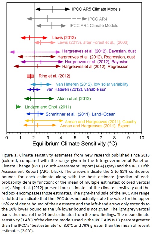
The determination of the global warming expected from a doubling of atmospheric carbon dioxide (CO2), called the climate sensitivity, is the most important parameter in climate science. The Intergovernmental Panel on Climate Change (IPCC) fifth assessment report (AR5) gives no best estimate for equilibrium climate sensitivity “because of a lack of agreement on values across assessed lines of evidence and studies.”
Studies published since 2010 indicates that equilibrium climate sensitivity is much less that the 3 °C estimated by the IPCC in its 4th assessment report. A chart here shows that the mean of the best estimates of 14 studies is 2 °C, but all except the lowest estimate implicitly assumes that the only climate forcings are those recognized by the IPCC. They assume the sun affects climate only by changes in the total solar irradiance (TSI). However, the IPCC AR5 Section7.4.6 says,
“Many studies have reported observations that link solar activity to particular aspects of the climate system. Various mechanisms have been proposed that could amplify relatively small variations in total solar irradiance, such as changes in stratospheric and tropospheric circulation induced by changes in the spectral solar irradiance or an effect of the flux of cosmic rays on clouds.”
Many studies have shown that the sun affects climate by some mechanism other than the direct effects of changing TSI, but it is not possible to directly quantify these indirect solar effects. All the studies of climate sensitivity that rely on estimates of climate forcings which exclude indirect solar forcings are invalid.
Fortunately, we can calculate climate sensitivity without an estimate of total forcings by directly measuring the changes to the greenhouse effect.
The greenhouse effect (GHE) is the difference in temperature between the earth’s surface and the effective radiating temperature of the earth at the top of the atmosphere as seen from space. This temperature difference is generally given as 33 °C, where the top-of-atmosphere global average temperature is about -18 °C and global average surface temperature is about 15 °C. We can estimate climate sensitivity by comparing the changes in the GHE to the changes in the CO2 concentrations.
The Clouds and Earth’s Radiant Energy System (CERES) experiment started collecting high quality top-of-atmosphere outgoing longwave radiation (OLR) data in March 2000. The last data available is June 2013 as of this writing on January 14, 2013. Figure 1 shows a typical CERES satellite.

Figure 1. CERES Satellite
The CERES OLR data presented by latitude versus time is shown in Figure 2.

Figure 2. CERES Outgoing Longwave Radiation, latitude versus date.
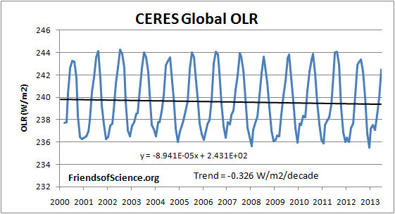
The global average OLR is shown in Figure 3.

Figure 3. CERES global OLR.
The CERES OLR data is converted to the effective radiating temperature (Te) using the Stefan-Boltzmann equation.
Te = (OLR/σ)0.25 – 273.15. where σ = 5.67 E-8 W/(m2K4), Te is in °C.
The monthly anomalies of the Te were calculated so that the annual cycle would not affect the trend.
We use the HadCRUT temperature anomaly indexes to represent the earth’s surface temperature (Ts). The HadCRUT3 temperature index shows a cooling trend of -0.002 °C/decade, and the HadCRUT4 temperature index shows a warming trend of 0.031 °C/decade during the period with CERES data, March 2000 to June 2013. The land measurement likely includes a warming bias due to uncorrected urban warming. The hadCRUT4 dataset added more coverage in the far north, where there has been the most warming, but failed to add coverage in the far south, where there has been recent cooling, thereby introducing a warming bias. We present results using both datasets.
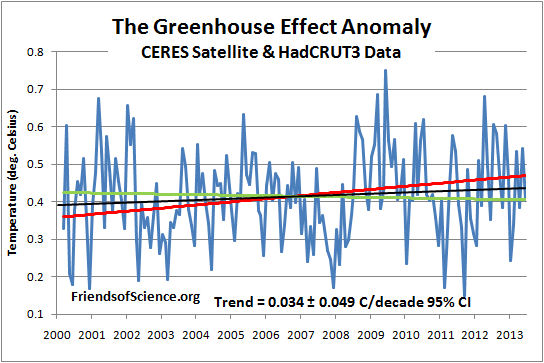
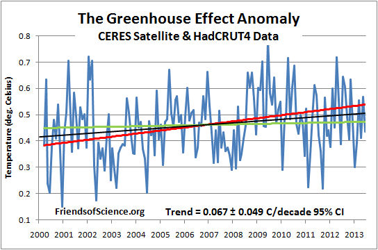
The difference between the surface temperatures anomaly and effective radiating temperature anomaly is the GHE anomaly. Figures 4 and 5 show the Greenhouse effect anomaly utilizing the HadCRUT3 and HadCRUT4 temperature indexes, respectively.

Figure 4. The greenhouse effect anomaly based on CERES OLR and HadCRUT3.

Figure 5. The greenhouse effect anomaly based on CERES OLR and HadCRUT4.
The trends of the GHE are 0.0343 °C/decade based on HadCRUT3, and 0.0672 °C/decade based on HadCRUT4.
We want to compare these trends in the GHE to changes in CO2 to determine the climate sensitivity. Only changes in anthropogenic greenhouse gases can cause a significant change in the greenhouse effect. Changes in the sun’s TSI, aerosols, ocean circulation changes and urban heating can’t change the GHE. Changes in cloudiness could change the GHE, but data from the International Satellite Cloud Climatology Project shows that the average total cloud cover during the period March 2000 to December 2009 changed very little. Therefore, we can assume that the measured change in the GHE is due to anthropogenic greenhouse gas emissions, which is dominated by CO2.
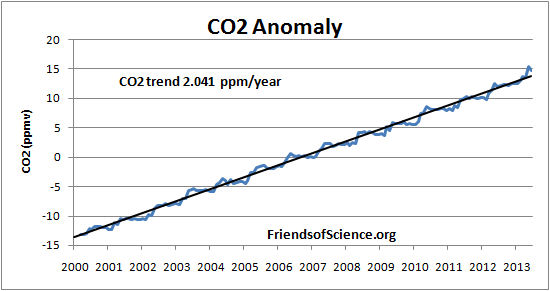
The CO2 data also has a large annual cycle, so the anomaly is used. Figure 6 shows the monthly CO2 anomaly calculated from the Mauna Loa data and the best fit straight line.

Figure 6. CO2 anomaly.
The March 2000 CO2 concentration is assumed to be the 13 month centered average CO2 concentration at March 2000, and the June 2013 value is that value plus the anomaly change from the fitted linear line. Table 1 below shows the CO2 concentrations, the logarithm of the CO2 concentration, and the change in the GHE from March 2000 for both the HadCRUT3 and HadCRUT4 cases.
Table 1 shows that the GHE has increased by 0.046 °C from March 2000 to June 2013 based on changes in the CERES OLR data and HadCRUT3 temperature data. Extrapolating to January 2100, the GHE increase to 0.28 °C by January 2100. Using the HadCRUT4 temperature data, the GHE increases by 0.55 °C by January 2100 compared to March 2000.
| hadCRUT3 | hadCRUT4 | |||
| Date | CO2 | Log CO2 | ΔGHE | ΔGHE |
| ppm | °C | °C | ||
| March 2000 | 368.88 | 2.567 | 0 | 0 |
| June 2013 | 395.94 | 2.598 | 0.046 | 0.089 |
| January 2100 | 572.68 | 2.758 | 0.283 | 0.554 |
| 2X CO2 | 737.76 | 2.868 | 0.446 | 0.873 |
Table 1. Extrapolated changes to the greenhouse effect (GHE) based on two versions of the hadCRUT datasets.
Table 1 shows that the GHE has increased by 0.046 °C from March 2000 to June 2013 based on changes in the CERES OLR data and HadCRUT3 temperature data. Extrapolating to January 2100, the GHE increase to 0.28 °C by January 2100. Using the HadCRUT4 temperature data, the GHE increases by 0.55 °C by January 2100 compared to March 2000.
The last row of Table 1 shows the transient climate response (TCR), which is the temperature response to CO2 emissions from March 2000 levels to the time when CO2 concentrations have doubled. TCR is less than the equilibrium climate sensitivity because the oceans have not reached temperature equilibrium at the time of CO2 doubling. TCR is calculated by the equation:
TCR = F2x dT/dF ; where dT means the temperature difference, dF means the forcing difference, from March 2000 to June 2013.
The CO2 forcing was calculated as 5.35 x ln (CO2/CO2i). The change in forcing from March 2000 to June 2013 is 0.379 W/m2. The forcing for double CO2 (F2x) is 3.708 W/m2. The TCR is 0.45 °C using hadCRUT3, and 0.87 °C using hadCRTU4 data. These values are much less than the multi-model mean estimate of 1.8 °C for TCR given in Table 9.5 of the AR5. The climate model results do not agree with the satellite and surface data and should not be used to set public policies.
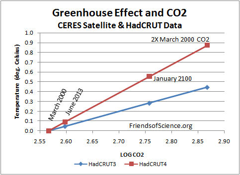
Figure 7 shows the results of Table 1 graphically.

Figure 7. The greenhouse effect and CO2 extrapolated to January 2100 and double CO2 bases on CERES and HadCRUT data.
This analysis suggests that the temperature change from June 2013 to January 2100 due to increasing CO2 would be 0.24 °C (from HadCRUT3) or 0.46 °C (from HadCRUT4), assuming the CO2 continues to increase along the recent linear trend.
An Excel spreadsheet with the data, calculations and graphs is here.
HadCRUT3 data is here.
HadCRUT4 data is here.
Mauna Loa CO2 data is here.
CERES OLR data is here.
Total cloud cover data is here.
A linear trend? Based on a 13-year period? In other words, projected far enough into the future, we will burn? This assumes everything remains constant, of course. As if nature is static and the climate never changes.
The 33 K GHE claim, originally from 1981_Hansen_etal.pdf (Google it) is baseless. This is because Hansen et al asserted with absolutely no evidence that the -18 deg C temperature for the radiative emitter in equilibrium with Space is a zone in the upper atmosphere.
This is not true: it is the flux-weighted average temperature of three main emitting zones; the surface at 15 deg C via the ‘atmospheric window’, the lower troposphere for H2O bands and -50 deg C for the CO2 15 micron band in the owed stratosphere.
The real GHE according to the same flat SW absorber/spherical LW emitter model is ~11 K. Hansen et al ‘forgot’ that if you remove GHGs from the atmosphere, no clouds or ice, SW increases by 43%.
So, there is no 3x positive feedback. In reality the atmosphere self-controls by changing OLR nature to compensate for pCO2 change, also net insolation change as cloud area and albedo vary.
Furthermore, no professional scientist or Engineer can accept that the Earth’s surface emits net IR energy at the black body level. Unfortunately, Meteorology and Climate Alchemy teach incorrect physics, including that a pyrgeometer outputs a real energy flux when it is the Radiation Field, a potential flux to a sink at 0 deg. C: only the difference of RFs transfers energy.
Also the sign of the effect of aerosols on cloud albedo is wrong – this is because Sagan’s aerosol optical physics failed to consider a second optical effect, easily proved experimentally by the ‘Glory’ phenomenon.
Therefore, Climate Science needs to be restarted under new management with no investment in incorrect science so as to correct these major errors (there are many more including failure in interpret Tyndall’s Experiment – there can be no gas phase thermalisation of absorbed IR energy).
Only then can the excellent experimentalists such as those operating CERES get the correct platform to present their data, instead of being under essentially political control.
For comparison has anybody done RSS and UAH?
@ur momisugly Katherine, that’s linear trend in CO2 increase, so yes liner trend is correct.
Any chance of an essay expanding on and consolidating all @AlecM’s points? That would be really useful!
@Peter Ward: in the mill. Climate Alchemy has been on the wrong track since Carl Sagan made 3 major physics’ mistakes leading him to conclude, wrongly, that GHGs cause Lapse Rate warming (it’s actually gravity).
I see even now Physicists assume the atmosphere is a grey-body emitter/absorber of IR energy – it’s really semi-transparent which is why OLR has been badly misinterpreted.
Katherine says: January 16, 2014 at 12:28 am
The dataset is short, so the extrapolation is uncertain, but it is the best dataset we have. The calculated transient climate response is the estimated effect of increasing greenhouse gases only. The small warming effect of CO2 can be easily be offset by natural climate change. We believe that the sun is a major driver of climate changes based on long-term correlations between solar activity and temperatures, so yes, temperatures might not increase for many years if solar activity remains low. The advantage of this direct calculation of changes in the greenhouse effect over the CERES era is that we do not need knowledge of total forcings or feedbacks.
garymount says: January 16, 2014 at 12:49 am
@ur momisugly Katherine, that’s linear trend in CO2 increase, so yes liner trend is correct.
_______________________________
But isn’t CO2’s absorption of LW inversely logarithmic, did I hear? i.e.: its ability to absorb maxes out at 500 ppm or something? I would be grateful for clarification on that.
But if so, then the absorption is not linear, even if the increase in concentration is.
Purely gravitational lapse rates are refuted by this essay. If the lapse rate were due to gravity, it would be possible to create a perpetual motion machine powered by said gravity.
http://wattsupwiththat.com/2012/01/24/refutation-of-stable-thermal-equilibrium-lapse-rates/
AlecM says: January 16, 2014 at 12:43 am
Silver Ralph says: January 16, 2014 at 1:38 am
Yes, the CO2 absorption of LW is logarithmic. That means it does NOT max out at 500 ppm.
See Figure 7. It is a graph of temperature versus the LOG of CO2 concentrations.
you cannot estimate radiative feedbacks (climate sensitivity) without knowing the radiative forcing(s), both natural and manmade. Forcings and feedbacks are intermingled in unknown proportions, and CERES measures the sum of both.
AlecM says: January 16, 2014 at 1:11 am
There must be some GHGs for there to be a lapse rate, ie, a decline of temperature with altitude to the tropopause. The value of the lapse rate does depend on gravity, which is not changing. An increase in GHG would cause the height of the tropopause to increase. Some data suggests that water vapor in the upper troposphere and lower stratosphere declines with increasing CO2, partially offsetting the CO2 direct effect, resulting in the low transient climate response I have calculated.
Climate models do not assume the atmosphere is a greybody. They are based on line-by-line code calculations that correctly simulates a semi-transparent atmosphere, ie, with an atmospheric window. But the climate models apparently greatly overestimates positive feedbacks from clouds and water vapor.
@Ken Gregory: “If there were no greenhouse gases in the atmosphere, but the same albedo, the surface would emit the 240 W/m2, and the average surface temperature would be about -18 C.”
Correct but very misleading, I wonder why?
If there were no greenhouse gases in the atmosphere, there would be no clouds or ice hence the SW thermalised at the surface would by definition be up to 43% higher. That would make the average surface radiative equilibrium temperature with Space of the flat SW absorber/spherical LW emitter 4 to 5 deg. C, a GHE of ~11 K. Thus the 3x ‘positive feedback’ is imaginary, a result of a rash assumption not picked up by peer review in 1981 and on which all the predictions of catastrophic warming are based.
Thus, to achieve 33 K GHE in the climate modelling, IR absorption in the atmosphere is increased over reality by a factor of 157.5/23 = 6.85x. If necessary, I can describe to readers how this numerical prestidigitation works (it involves another bit of incorrect physics). The hypothetical evaporation of sunlit oceans rises, hence the ‘positive feedback’, but the average atmospheric temperature also increases.
In 2010, US cloud physicist G L Stephens remarked that this temperature increase is corrected in the climate models during hind-casting, with no publicity, by using double real low level cloud optical depth, about 25% albedo increase. Because of this, the IPCC climate models cannot predict climate. It’s time to stop this farrago.
I’ve got a number of problems with this essay, as have some others. The timescale is surely too short for drawing any conclusions, especially as those conclusions depend on linear extrapolation of the small difference between two larger values. The CO2 effect appears to be treated as global, while the IPCC report makes it clear that its effect is concentrated mainly in the tropical troposphere [AR4 fig 9.1]. The essay asserts that “Changes in the sun’s TSI, aerosols, ocean circulation changes and urban heating can’t change the GHE“, but can they affect these calcs?- eg. GHE is being estimated using measured OLR as one of the inputs, OLR includes reflected LR, so would change if TSI changed. Maybe the other factors have the potential to affect the result too?
If all of the above issues are able to be dismissed, then one way of testing would be to select some subsets of the data period and apply the same calcs to each. Variation between results could indicate that the results are not reliable.
Ken Gregory:
I like your results so I wish I could accept them, but I cannot.
You say
Yes, and you say of your analysis
This finding agrees with other direct analyses which suggest ~0.4°C global temperature rise for a doubling of atmospheric CO2; e.g.
Idso from surface measurements
http://www.warwickhughes.com/papers/Idso_CR_1998.pdf
and Lindzen & Choi from ERBE satellite data
http://www.drroyspencer.com/Lindzen-and-Choi-GRL-2009.pdf
and Gregory from balloon radiosonde data
http://www.friendsofscience.org/assets/documents/OLR&NGF_June2011.pdf
Hence, you can see why I like your results so I am tempted to accept your analysis, but the following explains why I do not accept it.
You say you analysed
And your error estimates for those trends are?
Please note that the trend values span zero.
You say
This implies that you think the difference between the trends of the data sets is a result of the methods used to compile the temperature data sets. And you strengthen this implication saying
Sorry, but I do not agree.
The trends are not statistically significant from zero at 95% confidence because of the variances of the data sets. Your analysed “trends” are provided by random noise in the data. For your results to be valid they should be obtained from the extreme values allowed by the confidence limits of the trend lines (at 95% confidence). This would increase the spread of indicated global temperature rise projections to January 2100 to be greater than the 0.24 °C to 0.46 °C.
A result which is compiled from the variance of its analysed data is not valid.
I think your analysis provides a correct conclusion but that conclusion is obtained by analysis of apparent trends which result from the inherent errors in the data set. If your trend values were the extreme values allowed by the confidence limits of the trend lines (at 95% confidence) then your result would be valid. So, if I were asked to peer review your paper as reported above then I would commend that it not be accepted for publication. Sorry.
Richard
Two mysteries:
1) If the CO2 increase is largely anthropogenic as claimed by the IPCC, why does Figure 6 show no evidence of the decrease in consumption in much of the world after the 2008 financial crisis?
2) Why does AlexM repeat the same claims on every thread that mentions the GHE despite being unable to convince anyone ever that he knows what he’s talking about?
Ken Gregory says:
January 16, 2014 at 1:37 am
The advantage of this direct calculation of changes in the greenhouse effect over the CERES era is that we do not need knowledge of total forcings or feedbacks.
Doesn’t this assume that changes in the unknown forcings will average out and remain constant? For example, if Svensmark’s cosmic ray theory is valid and there’s a spike in galactic cosmic rays, your direct calculation would require the various other forcings to adjust so that CO2’s effect dominates. But why should they?
Also, in your original post, you wrote, “Changes in cloudiness could change the GHE, but data from the International Satellite Cloud Climatology Project shows that the average total cloud cover during the period March 2000 to December 2009 changed very little. Therefore, we can assume that the measured change in the GHE is due to anthropogenic greenhouse gas emissions, which is dominated by CO2.” While the average total cloud cover may have changed very little, Willis’s posts have shown that where the clouds appear can have a marked difference in how much sunlight gets through to warm the Earth. A decrease in cloudiness over the tropics could be offset by cloudiness in the temperate or polar regions for a net change of zero to the average total cloud cover but an overall increase in energy input, so just because the average changed very little doesn’t mean clouds can be disregarded.
Ken Gregory says:
January 16, 2014 at 1:50 am
Figure 2 shows that CERES measures the outgoing longwave radiation (OLR) at 240 W/m2. We are not assuming that all of this originates from the atmosphere. Some is emitted directly from the surface through the atmospheric window. However, the 240 W/m2 observed from space corresponds to a blackbody temperature of -18.1 deg. Celsius. If there were no greenhouse gases in the atmosphere, but the same albedo, the surface would emit the 240 W/m2, and the average surface temperature would be about -18 C.
But if there were no greenhouse gases in the atmosphere, there wouldn’t be any water vapor and therefore no clouds. In which case, how could you expect to have the same albedo?
Ken,
You can only say that the average surface temperature is -18C if you assume the following;
1. The Earth is flat and not a sphere
2. There is no day/night cycle
3. The solar energy input is reduced by a factor of 4 from what it actually is at TOA.
Not a good basis to build any sort of analysis really …
There is no need of the GHE because the measured outgoing energy does not come from the surface but 5-6Km up in the atmosphere, ie., the cloud tops. Also the outgoing energy is from the whole planet surface but solar heating is on one hemisphere. This minor effect, the rotating planet with a day and night cycle, is ignored by the AR4 K&T energy balance graphic which assumed a flat non rotating earth. With reality in the equation the GHE is not necessary.( let alone the fact that it violates the laws of thermodynamics).
Dancing polar vortex and solar activity.
http://losyziemi.pl/niezwykly-taniec-wiru-polarnego-ktory-silnie-reaguje-na-aktywnosc-slonca#more-25893
Roy Spencer says: January 16, 2014 at 2:10 am
Roy, I am familiar with your work, and I am very aware that forcings and feedbacks are intermingled in unknown proportions. However, I am using CERES and HadCRUT to measure the change in the greenhouse effect. I make no estimate of total forcings or feedbacks.
I wrote, “The HadCRUT3 temperature index shows a cooling trend of -0.002 °C/decade, and the HadCRUT4 temperature index shows a warming trend of 0.031 °C/decade during the period with CERES data, March 2000 to June 2013.” Both are insignificant temperature trends, so there was no change in temperature, and there was no feedbacks during the period!
There may be natural and man-made forcings during the period such as ocean circulation changes and lower solar forcings, but these do not change the greenhouse effect, ie the difference between the surface temperature and the effective radiating temperature. If fact, there must be negative forcings during the period to cause the “pause” in global warming. Only changes in the greenhouse gases and clouds will change the greenhouse effect. The IPCC says cloud cover can change only by a temperature change, ie, a feedback, but there was no temperature change during the period. A change in cloud cover could potentially change the OLR, but the ISCCP data shows no significant change in total cloud cover during the period. I use changes in CO2 to represent all man-made GHGs.
The TCR = 3.71 W/m2 X (dT/dF), where the dT is the change in the greenhouse effect over the period, and dF is the corresponding change in greenhouse gas forcing over the period, which is the ONLY forcing that would cause the dT. TCR for the HadCRUT3 case is 0.45 C for double CO2.
@Ken Gregory: you are correct:; the radiation transfer modelling does not assume a grey body. Indeed, the RTM is about the only thing in Climate Alchemy I trust!
My comment about the grey body assumption is that it was used by Houghton, copying Sagan, to claim the GHE causes lapse rate warming. It doesn’t; gravity does. A recent paper from Brookhaven used a grey body assumption so this beast is still alive in atmospheric physics.
We now get to the ‘enhanced greenhouse effect’ and Sagan’s ‘Venusian thermal runaway’ transferred to the Earth. It came down to the idea that when temperature exceeds a critical level, water ceases to condense so pH2O increases at the same time as lapse rate nearly doubles.
The problem is that these calculations assume the planetary surface emits net IR energy at the black body level. No professional scientist or engineer can accept this. I have measured, experimentally, coupled convection and radiation in metallurgical plants, also in research. We invented GHG physics so know rather a lot about it.
Radiation fields interact vectorially so there can be no emission from equal temperature surface to atmosphere of IR energy in any self-absorbed GHG band. [There’s a new bit of physics here.] The concept of ‘forcing’ is plain wrong. Increased pGHG reduces net surface IR emission. In the absence of any other factor the surface temperature would increase, hence the 1.2 K CO2 climate sensitivity would be correct. However, other processes offset this temperature rise reducing real CO2 climate sensitivity; it’s probably <0.1K.
To summarise, in climate modelling the RTM works fine. However, the Big Mistake is to put in 333W/m^2 imaginary IR from the surface to the atmosphere, apparently offset by applying Kirchhoff's Law of Radiation at ToA. I have spoken to modellers attempting to justify this by crazy S-B calculations. They are absolutely wrong because 134.5 of the net 157.5 W/m^2 'Clear Sky Atmospheric Greenhouse Factor' is a perpetual motion machine of the 2nd kind, hence the need for arbitrary cooling in hind-casting, that cooling having been apparently hidden until 2010.
@Katherine
Katherine says: January 16, 2014 at 12:28 am
It is actually a logarithmic trend with CO2. So on that graph d(log(2C)) = DT(0.8) . So on that basis even if in the unlikely event that CO2 levels were to quadruple to 1100 ppm by say 2300 global temperatures would still only rise by 1.6C. That is assuming the analysis is correct.
@ur momisugly Silver Ralph, I was talking of measured quantity, not its effect. It is my best guess that business as usual with emissions will be the best method of determining climate sensitivity to forcing in the shortest time possible. This would be the best policy for governments for the sake of the children ™.