Climate Dialogue about the (missing) hot spot
by Marcel Crok
Over at the Climate Dialogue website we start with what could become a very interesting discussion about the so-called tropical hot spot. Climate models show amplified warming high in the tropical troposphere due to greenhouse forcing. However data from satellites and weather balloons don’t show much amplification. What to make of this? Have the models been ‘falsified’ as critics say or are the errors in the data so large that we cannot conclude much at all? And does it matter if there is no hot spot?
The (missing) tropical hot spot is one of the long-standing controversies in climate science. In 2008 two papers were published, one by a few scientists critical of the IPCC view (Douglass, Christy, Pearson and Singer) and one by Ben Santer and sixteen other scientists. We have participants from both papers. John Christy is the ‘representative’ from the first paper and Steven Sherwood and Carl Mears are ‘representatives’ of the second paper.
Below I repost the introduction that we – the editors of Climate Dialogue – prepared as the basis for the discussion.
The (missing) hot spot in the tropics
Based on theoretical considerations and simulations with General Circulation Models (GCMs), it is expected that any warming at the surface will be amplified in the upper troposphere. The reason for this is quite simple.
More warming at the surface means more evaporation and more convection. Higher in the troposphere the (extra) water vapour condenses and heat is released. Calculations with GCMs show that the lower troposphere warms about 1.2 times faster than the surface. For the tropics, where most of the moist is, the amplification is larger, about 1.4.
This change in thermal structure of the troposphere is known as the lapse rate feedback. It is a negative feedback, i.e. attenuating the surface temperature response due to whatever cause, since the additional condensation heat in the upper air results in more radiative heat loss.
IPCC published the following figure in its latest report (AR4) in 2007:

Source: http://www.ipcc.ch/publications_and_data/ar4/wg1/en/figure-9-1.html (based on Santer 2003)
The figure shows the response of the atmosphere to different forcings in a GCM. As one can see, over the past century, the greenhouse forcing was expected to dominate all other forcings. The expected warming is highest in the tropical troposphere, dubbed the tropical hot spot.
The discrepancy between the strength of the hot spot in the models and the observations has been a controversial topic in climate science for almost 25 years. The controversy [i] goes all the way back to the first paper of Roy Spencer and John Christy [ii] about their UAH tropospheric temperature dataset in the early nineties. At the time their data didn’t show warming of the troposphere. Later a second group (Carl Mears and Frank Wentz of RSS) joined in, using the same satellite data to convert them into a time series of the tropospheric temperature. Several corrections, e.g. for the orbital changes of the satellite, were made in the course of years with a warming trend as a result. However the controversy remains because the tropical troposphere is still showing a smaller amplification of the surface warming which is contrary to expectations.
Positions
Some researchers claim that observations don’t show the tropical hot spot and that the differences between models and observations are statistically significant [iii]. On top of that they note that the warming trend itself is much larger in the models than in the observations (see figure 2 below and also ref. [iv]). Other researchers conclude that the differences between the trends of tropical tropospheric temperatures in observations and models are statistically not inconsistent with each other [v]. They note that some radiosonde and satellite datasets (RSS) do show warming trends comparable with the models (see figure 3 below).
The debate is complex because there are several observational datasets, based on satellite (UAH and RSS) but also on radiosonde measurements (weather balloons). Which of the dataset is “best” and how does one determine the uncertainty in both datasets and model simulations?
The controversy flared up in 2007/2008 with the publications of two papers [vi][vii] of the opposing groups. Key graphs in both papers are the best way to give an impression of the debate. First Douglass et al. came up with the following graph showing the disagreement between models and observations:

Figure 2. Temperature trends for the satellite era. Plot of temperature trend (°C/decade) against pressure (altitude). The HadCRUT2v surface trend value is a large blue circle. The GHCN and the GISS surface values are the open rectangle and diamond. The four radiosonde results (IGRA, RATPAC, HadAT2, and RAOBCORE) are shown in blue, light blue, green, and purple respectively. The two UAH MSU data points are shown as gold-filled diamonds and the RSS MSU data points as gold-filled squares. The 22-model ensemble average is a solid red line. The 22-model average ±2σSE are shown as lighter red lines. MSU values of T2LT and T2 are shown in the panel to the right. UAH values are yellow-filled diamonds, RSS are yellow-filled squares, and UMD is a yellow-filled circle. Synthetic model values are shown as white-filled circles, with 2σSE uncertainty limits as error bars. Source: Douglass et al. 2008
Santer et al. criticized Douglass et al. for underestimating the uncertainties in both model output and observations and also for not showing all radiosonde datasets. They came up with the following graph:

Figure 3. Vertical profiles of trends in atmospheric temperature (panel A) and in actual and synthetic MSU temperatures (panel B). All trends were calculated using monthly-mean anomaly data, spatially averaged over 20 °N–20 °S. Results in panel A are from seven radiosonde datasets (RATPAC-A, RICH, HadAT2, IUK, and three versions of RAOBCORE; see Section 2.1.2) and 19 different climate models. The grey-shaded envelope is the 2σ standard deviation of the ensemble-mean trends at discrete pressure levels. The yellow envelope represents 2σSE, DCPS07’s estimate of uncertainty in the mean trend. The analysis period is January 1979 through December 1999, the period of maximum overlap between the observations and most of the model 20CEN simulations. Note that DCPS07 used the same analysis period for model data, but calculated all observed trends over 1979–2004. Source: Santer (2008)
The grey-shaded envelope is the 2σ standard deviation of the ensemble-mean trends of Santer et al. while the yellow band is the estimated uncertainty of Douglass et al. Some radiosonde series in the Santer graph (like the Raobcore 1.4 dataset) show even more warming higher up in the troposphere than the model mean.
Updates
Not surprisingly the debate didn’t end there. In 2010 McKitrick et al. [viii] updated the results of Santer (2008), who limited the comparison between models and observations to the period 1979-1999, to 2009. They concluded that over the interval 1979–2009, model projected temperature trends are two to four times larger than observed trends in both the lower troposphere and the mid troposphere and the differences are statistically significant at the 99% level.
Christy (2010)[ix] analysed the different datasets used and concluded that some should be discarded in the tropics:

Figure 4. Temperature trends in the lower tropical troposphere for different datasets and for slightly differing periods (79-05 = 1979-2005). UAH and RSS are the estimates based on satellite measurements. HadAt, Ratpac, RC1.4 and Rich are based on radiosonde measurements. C10 and AS08 [x] are based on thermal wind data. The other three datasets give trends at the surface (ERSST being for the oceans only while the other two combine land and ocean data). Source: Christy (2010)
Christy (2010) concluded that part of the tropical warming in the RSS series is spurious. They also discarded the indirect estimates that are based on thermal wind. Not surprisingly Mears (2012) disagreed with Christy’s conclusion about the RSS trend being spurious writing that “trying to determine which MSU [satellite] data set is “better” based on short-time period comparisons with radiosonde data sets alone cannot lead to robust conclusions”.[xi]
Scaling ratio
Christy (2010) also introduced what they called the “scaling ratio”, the ratio of tropospheric to surface trends and concluded that these scaling ratios clearly differ between models and observations. Models show a ratio of 1.4 in the tropics (meaning troposphere warming 1.4 times faster than the surface), while the observations have a ratio of 0.8 (meaning surface warming faster than the troposphere). Christy speculated that an alternate reason for the discrepancy could be that the reported trends in temperatures at the surface are spatially inaccurate and are actually less positive. A similar hypothesis was tested by Klotzbach (2009).[xii]
In an extensive review article about the controversy published in early 2011 Thorne et al. ended with the conclusion that “there is no reasonable evidence of a fundamental disagreement between tropospheric temperature trends from models and observations when uncertainties in both are treated comprehensively”. However in the same year Fu et al.[xiii] concluded that while “satellite MSU/AMSU observations generally support GCM results with tropical deep‐layer tropospheric warming faster than surface, it is evident that the AR4 GCMs exaggerate the increase in static stability between tropical middle and upper troposphere during the last three decades”. More papers then started to acknowledge that the consistency of tropical tropospheric temperature trends with climate model expectations remains contentious.[xiv][xv][xvi][xvii]
Climate Dialogue
We will focus the discussion on the tropics as the hot spot is most pronounced there in the models. Core questions are of course whether we can detect/have detected a hot spot in the observations and if not what are the implications for the reliability of GCMs and our understanding of the climate?
Specific questions
1) Do the discussants agree that amplified warming in the tropical troposphere is expected?
2) Can the hot spot in the tropics be regarded as a fingerprint of greenhouse warming?
3) Is there a significant difference between modelled and observed amplification of surface trends in the tropical troposphere (as diagnosed by e.g. the scaling ratio)?
4) What could explain the relatively large difference in tropical trends between the UAH and the RSS dataset?
5) What explanation(s) do you favour regarding the apparent discrepancy surrounding the tropical hot spot? A few options come to mind: a) satellite data show too little warming b) surface data show too much warming c) within the uncertainties of both there is no significant discrepancy d) the theory (of moist convection leading to more tropospheric than surface warming) overestimates the magnitude of the hotspot
6) What consequences, if any, would your explanation have for our estimate of the lapse rate feedback, water vapour feedback and climate sensitivity?
[i] Thorne, P. W. et al., 2011, Tropospheric temperature trends: History ofan ongoing controversy. WIRES: Climate Change, 2: 66-88
[ii]Spencer RW, Christy JR. Precise monitoring of global temperature trends from satellites. Science 1990, 247:1558–1562.
[iii] Christy, J. R., B. M. Herman, R. Pielke Sr., P. Klotzbach, R. T. McNider, J. J. Hnilo, R. W. Spencer, T. Chase, and D. H. Douglass (2010), What do observational datasets say about modeled tropospheric temperature trends since 1979?, Remote Sens., 2, 2148–2169, doi:10.3390/rs2092148.
[iv]http://www.drroyspencer.com/wp-content/uploads/CMIP5-73-models-vs-obs-20N-20S-MT-5-yr-means1.png
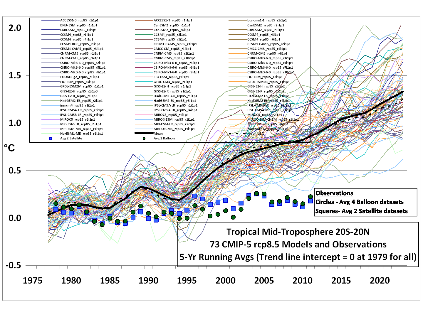
[v]Thorne, P.W. Atmospheric science: The answer is blowing in the wind. Nature Geosci. 2008, doi:10.1038/ngeo209
[vi] Douglass DH, Christy JR, Pearson BD, Singer SF. A comparison of tropical temperature trends with model predictions. Int J Climatol 2008, 27:1693–1701
[vii] Santer, B.D.; Thorne, P.W.; Haimberger, L.; Taylor, K.E.; Wigley, T.M.L.; Lanzante, J.R.; Solomon, S.; Free, M.; Gleckler, P.J.; Jones, P.D.; Karl, T.R.; Klein, S.A.; Mears, C.; Nychka, D.; Schmidt, G.A.; Sherwood, S.C.; Wentz, F.J. Consistency of modelled and observed temperature trends in the tropical troposphere. Int. J. Climatol. 2008, doi:1002/joc.1756
[viii] McKitrick, R. R., S. McIntyre and C. Herman (2010) “Panel and Multivariate Methods for Tests of Trend Equivalence in Climate Data Sets.” Atmospheric Science Letters, 11(4) pp. 270-277, October/December 2010 DOI: 10.1002/asl.290
[ix] Christy, J. R., B. M. Herman, R. Pielke Sr., P. Klotzbach, R. T. McNider, J. J. Hnilo, R. W. Spencer, T. Chase, and D. H. Douglass (2010), What do observational datasets say about modeled tropospheric temperature trends since 1979?, Remote Sens., 2, 2148–2169, doi:10.3390/rs2092148
[x] Allen RJ, Sherwood SC. Warming maximum in the tropical upper troposphere deduced from thermal winds. Nat Geosci 008, 1:399–403
[xi] Mears, C. A., F. J. Wentz, and P. W. Thorne (2012), Assessing the value of Microwave Sounding Unit–radiosonde comparisons in ascertaining errors in climate data records of tropospheric temperatures, J. Geophys. Res., 117, D19103, doi:10.1029/2012JD017710
[xii] Klotzbach PJ, Pielke RA Sr., Pielke RA Jr., Christy JR, McNider RT. An alternative explanation for differential temperature trends at the surface and in the lower troposphere. J Geophys Res 2009, 114:D21102. DOI:10.1029/2009JD011841
[xiii] Fu, Q., S. Manabe, and C. M. Johanson (2011), On the warming in the tropical upper troposphere: Models versus observations, Geophys. Res. Lett., 38, L15704, doi:10.1029/2011GL048101
[xiv] Seidel, D. J., M. Free, and J. S. Wang (2012), Reexamining the warming in the tropical upper troposphere: Models versus radiosonde observations, Geophys. Res. Lett., 39, L22701, doi:10.1029/2012GL053850
[xv] Po-Chedley, S., and Q. Fu (2012), Discrepancies in tropical upper tropospheric warming between atmospheric circulation models and satellites, Environ. Res. Lett
[xvi] Benjamin D. Santer, Jeffrey F. Painter, Carl A. Mears, Charles Doutriaux, Peter Caldwell, Julie M. Arblaster, Philip J. Cameron-Smith, Nathan P. Gillett, Peter J. Gleckler, John Lanzante, Judith Perlwitz, Susan Solomon, Peter A. Stott, Karl E. Taylor, Laurent Terray, Peter W. Thorne, Michael F. Wehner, Frank J. Wentz, Tom M. L. Wigley, Laura J. Wilcox, and Cheng-Zhi Zou, Identifying human influences on atmospheric temperature, PNAS 2013 110 (1) 26-33; published ahead of print November 29, 2012, doi:10.1073/pnas.1210514109
[xvii] Thorne, P. W., et al. (2011), A quantification of uncertainties in historical tropical tropospheric temperature trends from radiosondes, J. Geophys. Res., 116, D12116, doi:10.1029/2010JD015487
Mass, gravity and insolation set the base level of system energy content for any planet with an atmosphere.
Everything else that might try to alter that base level simply results in atmospheric circulation changes (atmosphere includes oceans for this purpose) that adjust the rate of conversion between kinetic and potential energy so as to keep the base level of system energy content stable.
That ‘everything else’ is actually all the complex variations that arise from the materials contained within the system whether Earth, oceans or atmosphere.
Composition changes, whether in the Earth, oceans or atmosphere can only affect circulation and not system energy content.
More potential energy and less kinetic energy allows more retention of energy because potential energy cannot radiate out.
Less potential energy and more kinetic energy allows more loss of energy because kinetic energy can radiate out.
In every situation where any sort of composition change seeks to disturb the base level of energy the reconfiguration of the circulation results in an instant equal and opposite thermal response via the exchange of PE for KE and vice versa.
The net effect is system stability despite composition variations.
Clarification of this point is required:
“Latent heat is removed prior to condensation by the conversion of kinetic energy to potential energy as the molecules rise against gravity to a region of lower pressure.”
Heat (not latent heat) is removed prior to condensation by conversion of kinetic energy to potential energy which then provokes condensation and when the phase change occurs the release of latent heat causes the air parcel to rise a little further with additional conversion of KE to PE until it reaches the correct lapse rate temperature for its height and then it stops rising and begins to descend.
One can see that in operation in convective cumulus towers. The uplift is energised when condensation occurs and the latent heat of the phase change is released.
Rather than the released latent heat being radiated to space the additional uplift it causes converts the excess KE to PE until thermal balance is once more achieved at a higher level.
The transmission of energy through the atmosphere is at the speed of light, for that atmospheric density, so very nearly the speed in a vacuum. This very small reduction in speed makes no difference to temperatures of the atmosphere because times are so very short. What GHG’s actually do is to remove some of that incoming energy to increase their own kinetic energy and reduce that falling onto the surface. The main atmospheric gasses, O2 and N2 are heated by the kinetic transfer of energy from the GHG’s. This heat escapes to space.
” O2 and N2 are heated by the kinetic transfer of energy from the GHG’s”
Not entirely.
Most O2 and N2 heating starts at the surface with conduction and is raised upward by convection, becoming PE in the process.
“””””…..Stephen Wilde says:
July 18, 2013 at 1:00 am
George.e..smith is right.
Cooling must occur first for condensation to start.
That cooling is primarily a result of pressure reduction with height as per the Ideal Gas Laws whereby the reduction in pressure allows expansion, the gases become less dense and temperature falls resulting in condensation. …….”””””””
The cooling is primarily a result of the earth losing energy to space.
To the extent that the flow of “heat energy” is a part of that process, by means of conduction (collisions between molecules), and convection (physical transport of molecules), the second law insists that the natural direction of that flow is from “hot” to “cold”. Ergo, there must be a negative Temperature gradient in the atmosphere to get “heat energy” to propagate from the surface to the upper reaches of the atmosphere.
Ultimately, only EM radiation can export energy out of the earth atmosphere to space (ignoring satellite launches, and other minor massive ejecta for the nit pickers).
So the thermal energy transported to high altitudes, must be ultimately converted to Electro-magnetic radiation, in order to escape the planet. Now some energy has already escaped to space by radiation directly from the surface, and Trenberth insists that is only 40 Watts per square meter, or about 10 % of the roughly 390 W/m^2 corresponding to a 288 Kelvin black body spectrum.
So 90% of earth’s energy must be radiated from the upper atmosphere to space; which is far too cold to do that, even if it was a black body, which it isn’t.
And that 90% pretty much has to be emitted at the 15 micron CO2 LWIR band, since N2 and O2 and Ar don’t radiate. Well I suppose we have to kick in the H2O and O3 GHG bands as well.
But ! the inescapable conclusion is that only 10% of the earth’s radiant energy emission can be in a 288 K thermal emission spectrum from the earth surface, since the atmosphere can only radiate GHG bands.
So seen from outer space the earth radiation spectrum should be a small (10 % area) 288K thermal spectrum, overlaid with prominent GHG band spectra like CO2 15 micron peaks, and various water peaks, plus the Ozone 9.6 micron peak.
Well sadly, that isn’t what is observed. There are > NO < GHG spectral peaks in the external radiation spectrum of the earth.
There are ONLY GHG spectral DIPS in an otherwise BB like thermal continuum spectrum.
Either Trenberth's 40 W/m^2 is wrong, or else the atmosphere itself IS radiating a normal thermal spectrum appropriate to its Temperature.
You can't generate a black body like thermal spectrum, out of the resonance lines of molecular oscillation and vibration modes, or rotation modes.
The solar spectrum of the sun consists of a roughly black body like thermal continuum spectrum, peaking at around 0.5 microns wavelength (plotted on wavelength scale; not wave number) , and overlaid with the Fraunhoffer lines of either bright atomic spectral lines, due to elements in the sun, or dark atomic absorption lines, due to absorption of elements in the solar outer atmosphere. Well that's the 4-H club version of what gose on. Use your imagination or Dr Svalgaard to sanitize it for prime time.
The point being, that the resonance emissions / absorptions of atoms / ions are not being grossly smudged out by the ambient Temperature of the sun; they remain characteristic of the atomic species that radiate / absorb them.
Same thing must apply to earth , the line / band spectra of molecular resonances, are not smudged out by the atmospheric, or surface Temperatures.
The background thermal radiation continuum, is a consequence of thermal emissions from either the surface, or the atmosphere itself, as a direct consequence of their Temperatures; or both in concert.
The spectral spread of the earth emission is huge, enormous, compared to the puny line broadening that is conceivably possible, due to Temperature (Doppler) broadening, and Pressure / density (collision) broadening, of molecular resonance emission lines.
That spectral spread, is only possible due to the Planck radiation formula which seems to govern thermal emissions due to Temperature, based on the hypothetical ideal black body radiation concept, which posits an emission spectrum ranging from zero to infinite wavelength or frequency; excluding of course both end points.
Evidently, the Planck formula was re-derived by Bose based on his concept of Bose-Einstein statistics, that apply to Bosons (including photons), as distinct from the Fermi-Dirac statistics that apply to Fermions, or the Maxwell-Boltzmann statistics, that apply to assemblages of interacting (colliding) "particles". I'll let the Quantum Chromo / Electro- Dynamics folks, sanitize that for you.
I am surprised no-one has commented on WG1 in the Fifth Assessment. When I looked for a discussion of the tropical hotspot in ZOD, it was missing – there was just a great big gap between Middle Troposphere and Lower Stratosphere. Watts Up? I asked.
In FOD, there were little snippets of information, but nothing of any substance – so I blew a loud whistle and said “Heh! Something is missing!”
SOD arrived, and it was still absent. So I got cross:
“The whole of the debate about the problems of reconciling radiosonde data with GCM models is missing. Figure 10.7 in WG1 of AR4 showed a predicted heating of about 0.6 deg C per decade between 400 and 100hPa and -30 deg S to 30deg N. However, none of the data from satellites or radiosondes confirms anything like that rate of heating. Allen, Robert J. and Sherwood, Steven C. (2008) Warming maximum in the tropical upper troposphere deduced from thermal winds. Nature Geosci 1 (6), 399- 403, http://dx.doi.org/10.1038/ngeo208 note “Climate models and theoretical expectations have predicted that the upper troposphere should be warming faster than the surface. Surprisingly, direct temperature observations from radiosonde and satellite data have often not shown this expected trend,” for instance – and then go on to suggest biases in the data. Lanzante, John R., Melissa Free, 2008: Comparison of Radiosonde and GCM Vertical Temperature Trend Profiles: Effects of Dataset Choice and Data Homogenization. J. Climate, 21, 5417–5435.
doi: http://dx.doi.org/10.1175/2008JCLI2287.1 (Not quoted in SOD) note that even after homogenization “in general the observed trend profiles were more similar to one another than either was to the GCM profiles.” Singer, S Fred, (2011). Lack of Consistency Between Modeled and Observed Temperature Trends Energy & Environment, 22, 375-406 DOI – 10.1260/0958-305X.22.4.375 (Not quoted in SOD) drew attention to the fact that “The US Climate Change Science Program [CCSP, 2006] reported, and Douglass et al. [2007] and NIPCC [2008] confirmed, a “potentially serious inconsistency” between modeled and observed trends in tropical surface and tropospheric temperatures.” and noted further that “Santer’s key graph — misleadingly suggests an overlap between observations and modeled trends. His “new observational estimates” conflict with satellite data. His modeled trends are an artifact, merely reflecting chaotic and structural model uncertainties that had been overlooked. Thus the conclusion of “consistency” is not supportable and accordingly does not validate model-derived projections of dangerous anthropogenic global warming.” Douglass, D. H., Christy, J. R., Pearson, B. D. and Singer, S. F. (2008), A comparison of tropical temperature trends with model predictions. Int. J. Climatol., 28: 1693–1701. doi: 10.1002/joc.1651 (Not quoted in SOD) note “Model results and observed temperature trends are in disagreement in most of the tropical troposphere, being separated by more than twice the uncertainty of the model mean.” Titchner, Holly A., P. W. Thorne, M. P. McCarthy, S. F. B. Tett, L. Haimberger, D. E. Parker, 2009: Critically Reassessing Tropospheric Temperature Trends from Radiosondes Using Realistic Validation Experiments. J. Climate, 22, 465–485. doi: http://dx.doi.org/10.1175/2008JCLI2419.1 (Not quoted in SOD) note that “tropical tropospheric trends in the unadjusted daytime radiosonde observations, and in many current upper-air datasets, are biased cold, but the degree of this bias cannot be robustly quantified.” It was my clear understanding that the Assessment Report was to review the current literature – there are some notable omissions, as I have noted above. Moreover, I had understood that the Report was to give due weight to differences of opinion – instead, any reading of the present text leaves the clear impression that the debate is being studiously avoided rather than being addressed. And one thing my own review of the debate has brought home to me is that even the satellite data does not come near the predictions that were made in AR4 – the discrepancy between ALL data and the models is wide. This debate MUST be reflected in the text.”
I shall be interested to read the final text.
george e smith says:
July 18, 2013 at 12:57 pm
“So seen from outer space the earth radiation spectrum should be a small (10 % area) 288K thermal spectrum, overlaid with prominent GHG band spectra like CO2 15 micron peaks, and various water peaks, plus the Ozone 9.6 micron peak.
Well sadly, that isn’t what is observed. There are > NO < GHG spectral peaks in the external radiation spectrum of the earth."
Very good. So GHG's serve only toabsorb and re-emit the same photons over and over again, until about as much escape to space on these frequencies as would have without the GHG's directly from clouds / the surface.
I've been likening it to a fog for years now; it scatters the energy but neither absorbs nor net emits it.
johnmarshall says:
July 18, 2013 at 7:02 am
“The main atmospheric gasses, O2 and N2 are heated by the kinetic transfer of energy from the GHG’s. This heat escapes to space.”
Thermalization and dethermalization happen to equal amounts under localo thermalo equilibrium (Kirchhoff’s Law). IOW: O2 and N2 are heated, but return the kinetic energy to GHG’s which then re-emit the photons.
Alan D McIntire says:
July 17, 2013 at 7:28 pm
“I got the impression from Held and Soden’s model, (see figure 1, page 11)
http://www.met.tamu.edu/class/atmo629/Summer_2007/Week%204/Water%20Vapor%20Feedback.pdf
that the temperature should increase by a roughly constant amount all through the atmosphere if their global warming theory is correct.
The folks at “Real Climate” addressed the issue here in a theoretical explanation they later admitted was wrong:
[…]
I think the Held-Soden model and “Realclimate” explanations were wrong because they assumed
an atmosphere releasing all its radiation from a 255 K height.”
Their first mistake is that they assume the atmosphere to be hydrostatic (i.e. unable to expand; as in a pressure cooker).
I skimmed through the PDF. NOWHERE do they talk about AIR PRESSURE, vertical air movement is once mentioned where they state that water vapour rises etc.; no explanation is given whether or not the barometric equation is used (it is, in the models; it assumes hydrostasis and we KNOW that the atmosphere is not hydrostatic!)
Likewise the stupid explanation by realclimate starts out with “Imagine an atmosphere with multiple isothermal layers that only interact radiatively.”
Yes, that’s a nice Gedankenexperiment but we know it is false for the atmosphere of the Earth; so scratch the rest!
george e. smith said:
“The cooling is primarily a result of the earth losing energy to space.”
General global cooling, yes.
Cooling leading to local condensation in a rising column of air, no.
The former is radiative cooling and the amount that can occur is dependent on the proportion of total system energy content that is in the form of kinetic energy rather than potential energy at any given time.
The latter results from kinetic energy being converted to potential energy as warm air rises against the force of gravity in a convective column.
So proclaims the “there’s magic back & forth-isms goin’ own that mayuth caint see nor cownt!” wannabe.
You really need to get with the fact what you say’s easy to check.
Being shameless isn’t intellectual validity.
Bear that in mind, or you can be reminded in front of hundreds. If not thousands.
=====
davidmhoffer says:
July 16, 2013 at 10:15 pm
2) Can the hot spot in the tropics be regarded as a fingerprint of greenhouse warming?
No, nor can the absence of one be construed as lack thereof.
1&2- the ipcc believe so –
http://www.ipcc.ch/publications_and_data/ar4/wg1/en/ch8s8-6-3-1.html
box 8.1 states clearly “Under such a response, for uniform warming, the largest fractional change in water vapour, and thus the largest contribution to the feedback, occurs in the upper troposphere. In addition, GCMs find enhanced warming in the tropical upper troposphere, due to changes in the lapse rate (see Section 9.4.4). This further enhances moisture changes in this region, but also introduces a partially offsetting radiative response from the temperature increase, and the net effect of the combined water vapour/lapse rate feedback is to amplify the warming in response to forcing by around 50% (Section 8.6.2.3).”
as per the models- http://www.ipcc.ch/publications_and_data/ar4/wg1/en/figure-8-14.html
3/ it is clear the ipcc believes they are close enough, yet they are most certainly not eg-
http://meteora.ucsd.edu/~pierce/papers/Pierce_et_al_AIRS_vs_models_2006GL027060.pdf
where they find the models are clearly wrong using another different satellite than the other two that found the model so far out that they are not worth using, yet here they are still being used as the largest portion of the surface temp models that are used in predictions!
this says it all about the history of this-
http://www.john-daly.com/sonde.htm
Stephen Wilde says:
July 18, 2013 at 9:17 pm
“The latter results from kinetic energy being converted to potential energy as warm air rises against the force of gravity in a convective column.”
Stephen, how should that work in a thermodynamic way? It would reduce entropy. (Brownian motion is unordered; potential energy is not.)
As I understand the Ideal Gas Law, the temperature one measures depends on the density of the gas as less density means less collisions of individual molecules with the measuring apparatus, or IOW, less kinetic energy per volume unit of gas.
DirkH
As gas molecules move apart or rise higher within a gravitational field kinetic energy gets replaced by potential energy.
I did find authority for that not long ago but cannot immediately find it.
Potential energy replaces kinetic energy in a gas molecule both when the molecule rises higher in the gravitational field and when the gas molecules move further apart.
Since reducing pressure with height around a sphere allows more space between molecules
and between the molecules and the ground the molecules cool due to conversion of kinetic energy to potential energy.
No radiation involved except in the background as part of the wider picture. It is a mechanical process involving movement within a gravitiational field generated by a sphere.
DirkH
I am sure that everything at a temperature above 0K radiates heat even the non GHG’s. It is how those gasses get that energy in the first place that is important, whether directly from insolation as the GHG’s or from secondary processes like kinetic collision. It all results in energy radiating from earth.
johnmarshall says:
July 19, 2013 at 4:22 am
“DirkH
I am sure that everything at a temperature above 0K radiates heat even the non GHG’s. ”
A gas molecule cannot radiate as long as its energy is lower than the energy of a photon of the lowest emission line in its line spectrum. It cannot and does not emit a continuous blackbody spectrum. It can transfer kinetic energy to another molecule though, and through random collisions a small number of the molecules will reach the necessary energy to radiate.
O2 and N2 do have very weak absorption / emission lines in the LWIR range. Unlike CO2 or H2O these are a few spikes only, as the vibrating mode is only possible in a 3-atom molecule.
So, O2 and N2 do radiate a small amount of heat. But on their very narrow lines.
the earths spectrum is of an aprox blackbody of 210K to 310K. water vapour and co2 will always be radiating, however water vapour has a lot more emission lines within that range than co2. co2 has finer vibrational lines whereas water vapour has vibrational and rotational transistions making it absorb lower in the spectrum, but not as fine lines.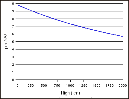
@Stephen Fisher wilde –
the change in gravity over our atmospheres height is virtually nothing, in fact in space it is still about 90% that of ground level.
A for what it is worth note:
The commonly held belief is thunderstorm clouds have a negatively charged base and a positively charged top.
A few years ago my husband edited a scientific paper for some Chinese scientists who used a field mill to determine the actual charges in thunderstorms. Instead of two zones as commonly thought the thunderstorm is a sandwich of three charged zones.
hmm, this statement –
“This change in thermal structure of the troposphere is known as the lapse rate feedback. It is a negative feedback, i.e. attenuating the surface temperature response due to whatever cause, since the additional condensation heat in the upper air results in more radiative heat loss.”
confuses the question as the main driver of the ‘thermal’ structural changes in the upper troposphere is not the lapse rate changes as such, it is the water vapour itself. the ipcc state-
“Under such a response, for uniform warming, the largest fractional change in water vapour, and thus the largest contribution to the feedback, occurs in the upper troposphere. In addition, GCMs find enhanced warming in the tropical upper troposphere, due to changes in the lapse rate (see Section 9.4.4). This further enhances moisture changes in this region, but also introduces a partially offsetting radiative response from the temperature increase, and the net effect of the combined water vapour/lapse rate feedback is to amplify the warming in response to forcing by around 50% (Section 8.6.2.3). The close link between these processes means that water vapour and lapse rate feedbacks are commonly considered together. The strength of the combined feedback is found to be robust across GCMs, despite significant inter-model differences, for example, in the mean climatology of water vapour (see Section 8.6.2.3). ”
where they clearly state that the overall response to the feedback is not negative, but positive by a large portion. if this were negative, the surface temp models would not predict a warming at all. the water vapour feedback would need to be offset completely by lapse rate feedback changes. the ipccs position/gcms position of this is-
http://www.ipcc.ch/publications_and_data/ar4/wg1/en/figure-8-14.html
where it is clear that water vapour feedback is MUCH stronger and counteracts the ‘lapse rate’ feedback. the two should be considered together as the ipcc considers and combined. they claim the tropospheric hot spot exists because more water vapour should exists in that region (raising of the upper troposphere), and small fractional changes make a larger change in the temperature anomaly because GHGs are in the lower part of the log scale rather that the higher saturated state. ie in the ipccs words-
“The radiative effect of absorption by water vapour is roughly proportional to the logarithm of its concentration, so it is the fractional change in water vapour concentration, not the absolute change, that governs its strength as a feedback mechanism. ”
from-
http://www.ipcc.ch/publications_and_data/ar4/wg1/en/ch8s8-6-3-1.html
the no show of the hot spot is proof that the models are WRONG. its as simple as that. they overstate the amplification by water vapour feedback by a large margin, and prove that feedback through other means (like clouds/rain) prevent the upper troposphere from warming. ie there is no runaway warming scenario possible, feedback is negative, and Cagw is rubbish.
@Mr. Crok –
your post should start with the ipcc position on this-
http://www.ipcc.ch/publications_and_data/ar4/wg1/en/ch8s8-6-3-1.html
box 8.1