Guest Post by Willis Eschenbach
“Climate sensitivity” is the name for the measure of how much the earth’s surface is supposed to warm for a given change in what is called “forcing”. A change in forcing means a change in the net downwelling radiation at the top of the atmosphere, which includes both shortwave (solar) and longwave (“greenhouse”) radiation.
There is an interesting study of the earth’s radiation budget called “Long-term global distribution of Earth’s shortwave radiation budget at the top of atmosphere“, by N. Hatzianastassiou et al. Among other things it contains a look at the albedo by hemisphere for the period 1984-1998. I realized today that I could use that data, along with the NASA solar data, to calculate an observational estimate of equilibrium climate sensitivity.
Now, you can’t just look at the direct change in solar forcing versus the change in temperature to get the long-term sensitivity. All that will give you is the “instantaneous” climate sensitivity. The reason is that it takes a while for the earth to warm up or cool down, so the immediate change from an increase in forcing will be smaller than the eventual equilibrium change if that same forcing change is sustained over a long time period.
However, all is not lost. Figure 1 shows the annual cycle of solar forcing changes and temperature changes.

Figure 1. Lissajous figure of the change in solar forcing (horizontal axis) versus the change in temperature (vertical axis) on an annual average basis.
So … what are we looking at in Figure 1?
I began by combining the NASA solar data, which shows month-by-month changes in the solar energy hitting the earth, with the albedo data. The solar forcing in watts per square metre (W/m2) times (1 minus albedo) gives us the amount of incoming solar energy that actually makes it into the system. This is the actual net solar forcing, month by month.
Then I plotted the changes in that net solar forcing (after albedo reflections) against the corresponding changes in temperature, by hemisphere. First, a couple of comments about that plot.
The Northern Hemisphere (NH) has larger temperature swings (vertical axis) than does the Southern Hemisphere (SH). This is because more of the NH is land and more of the SH is ocean … and the ocean has a much larger specific heat. This means that the ocean takes more energy to heat it than does the land.
We can also see the same thing reflected in the slope of the ovals. The slope of the ovals is a measure of the “lag” in the system. The harder it is to warm or cool the hemisphere, the larger the lag, and the flatter the slope.
So that explains the red and the blue lines, which are the actual data for the NH and the SH respectively.
For the “lagged model”, I used the simplest of models. This uses an exponential function to approximate the lag, along with a variable “lambda_0” which is the instantaneous climate sensitivity. It models the process in which an object is warmed by incoming radiation. At first the warming is fairly fast, but then as time goes on the warming is slower and slower, until it finally reaches equilibrium. The length of time it takes to warm up is governed by a “time constant” called “tau”. I used the following formula:
ΔT(n+1) = λ∆F(n+1)/τ + ΔT(n) exp(-1/ τ)
where ∆T is change in temperature, ∆F is change in forcing, lambda (λ) is the instantaneous climate sensitivity, “n” and “n + 1” are the times of the observations,and tau (τ) is the time constant. I used Excel to calculate the values that give the best fit for both the NH and the SH, using the “Solver” tool. The fit is actually quite good, with an RMS error of only 0.2°C and 0.1°C for the NH and the SH respectively.
Now, as you might expect, we get different numbers for both lambda_0 and tau for the NH and the SH, as follows:
Hemisphere         lambda_0     Tau (months)

    NH               0.08           1.9

    SH               0.04           2.4
Note that (as expected) it takes longer for the SH to warm or cool than for the NH (tau is larger for the SH). In addition, as expected, the SH changes less with a given amount of heating.
Now, bear in mind that lambda_0 is the instantaneous climate sensitivity. However, since we also know the time constant, we can use that to calculate the equilibrium sensitivity. I’m sure there is some easy way to do that, but I just used the same spreadsheet. To simulate a doubling of CO2, I gave it a one-time jump of 3.7 W/m2 of forcing.
The results were that the equilibrium climate sensitivity to a change in forcing from a doubling of CO2 (3.7 W/m2) are 0.4°C in the Northern Hemisphere, and 0.2°C in the Southern Hemisphere. This gives us an overall average global equilibrium climate sensitivity of 0.3°C for a doubling of CO2.
Comments and criticisms gladly accepted, this is how science works. I put my ideas out there, and y’all try to find holes in them.
w.
NOTE: The spreadsheet used to do the calculations and generate the graph is here.
NOTE: I also looked at modeling the change using the entire dataset which covers from 1984 to 1998, rather than just using the annual averages (not shown). The answers for lambda_0 and tau for the NH and the SH came out the same (to the accuracy reported above), despite the general warming over the time period. I am aware that the time constant “tau”, at only a few months, is shorter than other studies have shown. However … I’m just reporting what I found. When I try modeling it with a larger time constant, the angle comes out all wrong, much flatter.
While it is certainly possible that there are much longer-term periods for the warming, they are not evident in either of my analyses on this data. If such longer-term time lags exist, it appears that they are not significant enough to lengthen the lags shown in my analysis above. The details of the long-term analysis (as opposed to using the average as above) are shown in the spreadsheet.
KR:
Your post at May 30, 2012 at 11:50 am says:
You are right. I made a mistake.
Please accept my sincere apology. I did not intend the insult.
Richard
Philip Bradley:
re. your post at May 29, 2012 at 3:12 pm
Correlation is not proof of causation. Live with it.
Richard
Willis must be joking. This reasoning behind this calculation is pathetically foolish, and it would be laughed at, if it were submitted to a respectable journal..
The reaction of the earth’s climate to an influx of radiation cannot simply be characterized by a single time constant and a single heat capacity. There are a number of different time constants because there are a number of different mechanisms for the transfer of heat within the system. Some of the time constants are short like the daily heating and cooling of the surface of the land, and ocean, and others associated with deeper penetration of heat into the depths of the land and ocean are much longer. A short term oscillating radiation stimulus will only uncover the time constant associated with the shallowest penetration of heat into and out of the system.
A paper by Stephen Schwartz written in 2007 derived a single time constant of 5 years, looking at past data on the earth’s climate. He was forced to admit that even this estimate was incorrect and too small once he was confronted with the fact that his model was over simplistic. The longest time constant is more like 70 years according to many of the climate models.
I don’t see how people can call themselves skeptics and yet endorse such a simplistic and flawed analysis.
Andrew:
Your post at May 29, 2012 at 12:17 pm says;
I agree.
We seem to be starting a semantic argument about the meaning of “causation” which I am not willing to continue.
If it will help, I am willing to accept the amendment to my statement such that it becomes
“The absence of correlation disproves direct causation”.
If that is not acceptable to you then so be it. I am not willing to continue the matter whatever is said.
Richard
Willis,
By the way, I should make it clear that I am not criticizing you for trying to use the simplest model possible to try to learn what you can. As a physicist, I definitely like that sort of approach. However, it is important to recognize the caveat that one should always use the simplest model possible…but no simpler. I think the point here is that these one-box models with a single timescale are too simple for the purpose. In particular, although you can fit it well to data where the forcings are over a fairly narrow range of frequencies, more careful investigation shows that it is deficient…namely, that it will tend not to predict very well for data over a different range of frequencies than what you fit it over. This is why when you fit your model to the GISS model emulation of the instrumental temperature record, you could get a good result as long as you didn’t look at response to a forcing at a different frequency (like the volcanic forcing, or like the long-time response to a doubling of CO2 as is used to determine the equilibrium climate sensitivity).
This is also why you can again get a good result for fitting to the forcing due to the seasonal cycle but will no doubt find that if you use this result to predict the climate sensitivity in a full-fledged climate model, it will not give anything close to the correct result. (And, I would argue, it is likely not to give anything close to the correct result for the real world, although unfortunately we don’t know what the correct result is for the real world, since this is of course what we are trying to find out.)
The main reason, as I noted is the very different heat capacities and resulting timescales for response of the ocean mixed layer and of the atmosphere. (One probably has to worry also about the timescale for response of the deep ocean…But, two timescales would at least be a lot better than one.)
Joeldshore:
I am giving a partial answer to your post (at May 30, 2012 at 11:59 am) which is addressed to me because your post is so wrong I would need to write a book to answer all its errors.
You ask:
I answer:
If you don’t know the answer to that question then all your posts in this thread are pointless.
A flaw would be a significant error of understanding, assumption, calculation and/or interpretation.
If you cannot find a flaw or indicate how a flaw probably exists then don’t bother to critique his model.
You say
What is “strange” is your daft idea that I “believe” anything about Willis’ analysis or climate models.
I know of no flaw in Willis’ analysis although there may be several.
I know that all except at most one of the GCMs is wrong because they each use a different value of climate sensitivity.
Your assertions about my “beliefs” seem to be your psychological projection.
You assert
Your assertion demonstrates that you did not read Willis’ account of his analysis or you failed to understand it. There are no other possibilities.
You say
Clearly, you do not know or understand the difference between heuristic and predictive modelling.
Your suggestion that the climate sensitivity provided by Willis’ analysis should be checked against a climate model is plain daft. Which climate model? They each use a different value of climate sensitivity.
More fundamentally, as I told you, Willis is analysing reality. Any model is an expression of an understanding of reality.
Reality matters more than anybody’s understanding of it.
Therefore,
• it is reasonable to assess a model by comparison to the result of Willis’ analysis
but
• it cannot possibly be reasonable to assess the result of Willis’ analysis by comparison to a model.
Richard
Another problem with Willis’ article is that his calculation only includes solar forcing. It neglects the long wave radiation escaping upward into space, because the earth absorbs short wave radiation, and radiates most of what it absorbs upward as long wave radiation. This is different from the solar radiation that is directly reflected. All of the net flow of radiation counts as forcing. This seems to be another basic phenomenon neglected in Willis’ fatally flawed calculation.
I haven’t read all of the posts on this page. It would be very sad if nobody else reading this blog recognized how flawed this calculation is. All I have noticed so far is praise. This is very perplexing.
REPLY: It is not perplexing at all you are just being your usual concern troll self – Anthony
So you started with a bivariate time series in F and T, and created derived time series ΔT and ∆F by computing first differences. Then to half of the time series you estimated the linear vector autoregressive model ΔT(n+1) = a∆F(n+1) + bΔT(n). You introduced a third variable τ, and nonlinear functions a = a(τ) and b=b(τ). In your modeling, any nonlinear monotonic functions would do as well. Now ∆F(n+1) is correlated with ΔT(n), they differing is signs only at the solstices (lower left “corner” and upper right “corner), where ΔT changes sign a month after ∆F changes sign. If these had been the original data plotted in chronological order, they would be called “hysteresis” plots, and you’d see the individual years (unless you plotted using thick lines to hide them), but they seem to be the averages by month of year — is that so?
“Correlation usually implies causation” in the sense that, historically, when X and Y variables have been found reliably to be highly correlated they are usually related by a causal mechanism. However, correlation does not imply that changing X will change Y, or that changing Y will change X.
You have done several things that you usually deprecate: you took model output as data (this is what I asked you about); you worked with averages over large spatial and time scales; you assumed that change in temperature is a linear function of change in forcing; you assumed that the change in CO2 changes radiative forcing in the usual way assumed by climate theorists; you assumed that the system was stationary; and you reported the resultant estimate without an uncertainty or standard deviation estimate.
@ur momisugly George E. Smith
Re. Your comment to me of May 30, 2012 at 11:18 am
You tell me that I am ‘missing the whole point’. Actually, I think that is what you are doing.
The secondary emission from CO2 (which you described as taking place between notional thin sheets) does not affect my argument because that is only concerned with the absorption of radiant energy/power from the initial ‘beam’ radiating from the earth’s surface. The secondary emissions and their possible re-absorption by other CO2-molecules do not affect this substantially (since the probability of a re-emitted photon being intercepted by another CO2 molecule that was receptive to it would be extremely small in the earth’s atmosphere) and the primary absorption therefore follows the B-L law as per normal. If the absorbed photons are not really ‘dead’ I think they might as well be for all the difference it would make to the amount absorbed from the primary radiance.
Since the CO2 molecules are mixed up with all the other molecules comprising the atmosphere, once they have absorbed their portion of the primary outgoing radiance from the earth’s surface that absorbed power has then been effectively captured by the whole atmosphere whose overall mean temperature will be increased accordingly. At this somewhat higher mean temperature the atmosphere will radiate more strongly both to outer space and back to the surface. The amount being re-radiated back to the surface is what constitutes the ‘radiative forcing’ from CO2 in the techno-jargon of the IPCC. In the ideal condition of steady-state equilibrium the amount of this so-called ‘back-radiation’ will be a constant fraction of the amount initially absorbed by the CO2 from the primary surface radiance. This fraction is represented by the symbol ‘p’ in my formula derived from B-L, and is hidden invisibly in the number ‘5.35’ in the IPCC’s formula.
I have tried to address your points as fully as I can here because I’m about to go off on a trip and won’t be able to address any more before I get back in a couple of weeks.
KR says:
May 30, 2012 at 8:04 am
Many thanks for your pointers to interesting sites in your response to me and to Willis.
Willis asked for me to show how a diurnal cycle implies even lower sensitivity. Take an area like the Pacific, and its diurnal forcing cycle, maybe a few hundred to a thousand W/m2. Its diurnal temperature range is only about 1 degree. The sensitivity is therefore 0.001 to 0.01 degrees per W/m2, which extrapolates to about 0.004-0.04 degrees per CO2 doubling. What’s wrong with this, of course, is the high frequency of the diurnal cycle that doesn’t allow the ocean to adjust to those W/m2. Extending to a year suffers from underestimation for similar reasons. The same amplitude forcing applied on longer and longer frequencies will have a larger and larger responses, because the responses are limited by how the lag interacts with the frequency. You won’t get the full equilibrium response unless the forcing increases to a constant level and doesn’t reverse.
richardscourtney says: “I agree. We seem to be starting a semantic argument about the meaning of “causation” which I am not willing to continue.”
I can see you are frustratedly dealing with other people right now. I merely wanted to point out that to assume uncorrelated variables are independent is as fallacious as assuming causation is demonstrated by correlation.
Well, even if you aren’t interested, in case anyone else is:
A lack of correlation between two normally distributed random variables that are not known to be jointly normal may mean that they are independent (neither variable is related to the other) but if they aren’t jointly normal it doesn’t. If they aren’t jointly normal, all that can be said is that neither variable appears to be linearly dependent on the other, or in any way that might “look” linear to some extent, that is, if there is a casual relationship it must involve some other equation that relates them than a line or an equation that behaves vaguely like one, such as the relationships described at the link I gave above. Of course, it must be a relationship which would not create any apparent linear correlation so several relationships besides linear ones are also likely ruled out. Whether this is the same thing as saying direct causation is ruled out is not clear to me.
Willis Eschenbach says:
May 29, 2012 at 11:16 am
“Eric Adler says:
May 29, 2012 at 10:38 am
“This post is a joke right?
Climate is a complex system. Reducing the modeled time dependence to a single time constant based on an oscillating forcing is nonsense. A paper by Schwartz based on historical data estimated a single time constant of 5 years, and had to take it back. If there is a single time constant that could describe what is happening it is more like 80 years.”
Your comment is a joke, right?
I say that because claiming something is “nonsense”, with no attempt to even begin to tell us why it is “nonsense”, is a joke in the world of science. I may well be wrong, I have been many times, but you have not said one word about where or how I might have gone off the rails.
w.
PS—As far as I can find out, Schwartz didn’t “take it back”. He modified his estimate to make it ≈ 8 years.”
He revised his climate sensitivity so that a doubled CO2 concentration would yield a 1.9C temperature rise. He admitted that there was more than one time constant, and the shorter one, which was a few months, similar to yours, was not relevant for the estimation of equilibrium climate sensitivity,
http://www.ecd.bnl.gov/steve/pubs/HeatCapCommentResponse.pdf
“Revised determination of climate sensitivity. The upward revision of the climate system time constant
4 by approximately 70% results, by Eq (1), in a like upward increase in the value of the climate sensitivity
5 from the value given in S07, 0.30 ± 0.14 K/(W m-2) to 0.51 ± 0.26 K/(W m-2), corresponding for the
6 forcing of doubled CO2 taken as 3.7 W m-2, to an equilibrium increase in GMST for doubled CO2 ΔT2×
7 of 1.9 ± 1.0 K. Although this value is still rather low compared to many current estimates it is much
8 more consistent than the value given in S07 with the estimate given in the Fourth Assessment Report of
9 the IPCC [2007] as “2 to 4.5 K with a best estimate of about 3 K and … very unlikely to be less than 1.5
10 K”.
oops, above I wrote: Now ∆F(n+1) is correlated with ΔT(n), they differing is signs only at the solstices (lower left “corner” and upper right “corner), where ΔT changes sign a month after ∆F changes sign.
I forgot that these were deltas, though I wrote them. The places where ΔT changes sign a month after ∆F changes sign are at the Y intercepts, (.∆F = 0), not at the upper right and lower left extremal points of the ellipses.
Willis Eschenbach said @ur momisugly May 30, 2012 at 12:55 pm
How odd! That’s the same result that I get from MODTRAN.
Capo: “Willis, please could you explain your formula
 ,
, and
and  for all
  ,
,
 ,
,  , and
, and
 .
. seem to be treated the values the temperature assumes immediately after respective impulses:
 for all
  , i.e. in which
  for
for  and in which
  is a non-zero value small enough that the system can be considered linear.
 always equals
  before
  , so it is reasonable to assume that before
  the
the  ‘s had values at most negligibly different from
  –i.e., that before then the
  ‘s were negligible–since a time whereof the memory of man runneth not to the contrary.
 , though, the surface-temperature sample values
  begin to increase, asymptotically approaching a value at which the resultant change in radiation (and other heat) loss by the surface equals the change
  incoming radiation. I assume you will accept without proof that the approach to that value is exponential, with a time constant of, say,
  , which means that for
  ‘s such that
  :
:
 . (1)
. (1) , the limit it thereby approaches is
  , and, bearing in mind the initial slope of an exponential with time constant
  , we can conclude that the initial response
  of the temperature to the radiation-impulse increase is given by
 .
. such that
  :
:
 . (2)
. (2) and
and  are not in general zero:
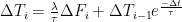
ΔT(n+1) = λ∆F(n+1)/τ + ΔT(n) exp(-1/ τ) ? Do you have any sources for that?”
That puzzles me, too. It seems to imply that Mr. Eschenbach thinks of the short-wave radiation as being delivered in a sequence of impulses:
where
Further, the temperature values
With those assumptions you could get something akin to Mr. Eschenbach’s equation by starting with a simplified scenario in which
In that scenario,
In response to the step change in radiation-impulse magnitudes at
If the incremental sensitivity of temperature to small changes in (incoming short-wave) radiation is
Reflection reveals that this relationship holds in general for any
Finally, linearity enables us to apply superposition to (1) to (2) to arrive at the following approximation to Mr. Eschenbach’s equation for situations in which
This differs from his in that I (harmlessly, I believe) displaced the indexing by one period and that I included a dimensioned numerator in the exponent to make the exponent dimensionless. Without having thought it through completely, I sense that in the context he’s using his equation he’ll arrive at a delay that’s about a half month too high, but that’s a quibble—and I haven’t proven to myself that it’s true.
Joe Born:
I am writing to ask for a clarifying statement concerning your post at May 31, 2012 at 5:37 am.
I follow the maths but I do not understand your point.
Your post begins by asking for an explanation of Willis’ equation and says;
“It seems to imply that Mr. Eschenbach thinks of the short-wave radiation as being delivered in a sequence of impulses”.
It then says;
“the temperature values T_i seem to be treated the values the temperature assumes immediately after respective impulses”
and concludes
“With those assumptions you could get something akin to Mr. Eschenbach’s equation by starting with a simplified scenario …”
OK. I get all that, but it seems your argument agrees the method Willis has adopted.
Are you disputing the assumptions which you state? They seem reasonable to me.
I note your point that in Willis’ model the surface temperature will rise exponentially until radiation loss from the surface increases to halt the surface temperature rise. But so what? That would seem to govern climate sensitivity, would it not? So, it seems that I am missing the point you are trying to make.
I could continue, but I have said sufficient to demonstrate that I have failed to understand the point you are making.
Hence, I would be grateful for a succinct statement of your substantive point. Thanking you in anticipation
Richard
As an expansion on this discussion, a two-box/two time constant model (as opposed to the one-box/single time constant model W. Eschenbach is using here) fit to forcings and the southern oscillation index (http://tinyurl.com/7t8rs8b) is quite capable of reproducing the observed temperatures. The estimated climate sensitivity from that slightly more complex model, one that that better matches the physics (fast responding atmosphere, slow responding oceans) is ~2.6C/doubling CO2.
The Pompous Git:
re. your comment at May 30, 2012 at 11:59 pm about the similarity of Willis’ result (which assesses total climate sensitivity) and your MODTRAN result.
That similarity would seem to suggest the water vapour feedback on climate sensitivity is zero (or close to zero).
Richard
richardscoutney (May 31, 2012 at 7:03 am):
That the data permits almost any interpretation one cares to make can be traced to a fundamental error in the construction of modern climatology. This is that the models reference no statistical population. Absent the associated population, the models cannot be tested.
KR:
Thankyou very much for your comment at May 31, 2012 at 6:27 am which says;
You point to a fundamental problem with most of climate science; viz.
the data permits almost any interpretation one wants to make.
Very recently (on another thread of WUWT) I have been involved in a discussion where an individual is certain his model of the carbon cycle must be ‘right’ because it fits the empirical data: his certainty is not altered by the fact that I have also modeled the carbon cycle in 6 other – and each different – ways and each of those models also matches the same data.
Your analysis provides a very different result from that of Wills, and that difference is because you and he use different assumptions. The problem is to determine which if either of those analyses is right.
All we can do is to try to falsify both your and Willis’ analyses. In this discussion we are trying to find fault with Willis’ analysis. Perhaps you could ask Anthony to publish your analysis on WUWT so we can attempt to perform the same service for you?
Richard
Joe Born,
thank you very much for your helpful comments. Ok, my problems with the units are solved, Delta_T is not the temperature anomaly referring to a initial state, it seems to be some sort of derivation of T in units °C/month. So the units are fitting on both sides.
Given your interpretation as true, the exciting question now is:
What is lambda in Willis’ formula? With regard to the short time intervals, it seems to be a “super-fast” climate sensitivity, where feedbacks have almost no time to get in. This could explain, why Willis’ value comes close to the climate sensitivity for CO2 only without feedbacks (about 1°C).
But I think there’s a further problem:
You wrote “which means that for i‘s such that \Delta F_i=0:
\Delta T_i=\Delta T_{i-1} e^{\frac{-\Delta t}{\tau}}”
Delta F_i=0 means, there is no further incremental step in forcing. But the system goes on getting warmer until the new eqilibrium temperature is reached. So why? Because the former incremental steps of forcing are still operating. It’s an effect which should be contributed to climate sensitity, but in Willis’ formula it gets separated from lambda and is put in the second term. Again, low values for lambda are not surprising any more. In my opinion Willis’ lambda is just a fit parameter, but it hasn’t the correct meaning of usual climate sensitivity.
Best regards
richardscourtney says:
May 31, 2012 at 7:03 am
KR:
Thankyou very much for your comment at May 31, 2012 at 6:27 am which says;
….
“Your analysis provides a very different result from that of Wills, and that difference is because you and he use different assumptions. The problem is to determine which if either of those analyses is right.
All we can do is to try to falsify both your and Willis’ analyses. In this discussion we are trying to find fault with Willis’ analysis. Perhaps you could ask Anthony to publish your analysis on WUWT so we can attempt to perform the same service for you?
Richard”
Richard,
There are a number of scientific points which have been made against Willis’ post here and have not been addressed by Willis or anyone else.
1) A model with a single time constant is clearly inadequate to describe the climate of the earth. It should have at least two time constants to describe the radically different characteristics of energy absorption by the ocean and atmosphere. This point was made in KR’s link to Tamino’s empirical analysis of the response of the global temperature to long and short duration forcings.
There is no need to publish this material on WUWT. It is freely available to any reader here, including Willis.
http://web.archive.org/web/20100104073232/http://tamino.wordpress.com/2009/08/17/not-computer-models/
It is clear that the effects of the longer time constant involving temperature change of the ocean, over the long term, will not appear in the analysis if you are only looking at annual variations in forcing or other short term data like volcanic eruptions. That is why a two box model, rather than a one box model is used. In a previous post I pointed out that Stephen Schwartz also erroneously used a 1 box model in his paper, but when this was pointed out to him, he corrected himself. The climate sensitivity he derived was 1.9C for a doubling of CO2.
2)Willis seems to have been looking at only on forcing component, arriving solar radiation, minus the reflected radiation. This does not represent all of the forcing components needed to explain the evolution of climate.
If no answer to these criticisms is presented, it would appear that there are none.
richardscourtney – “…the data permits almost any interpretation one wants to make”
I would have to disagree. Eschenbach’s one-box model (which appears to be based upon or quite similar to Schwartz model) produces widely different results when looking at forcings of different time scales – such as seasonal, CO2, volcanic, etc. And in fact when looking at longer term forcings (http://wattsupwiththat.com/2011/05/14/life-is-like-a-black-box-of-chocolates/) Eschenbach had to introduce an arbitrary scaling factor to the volcanic forcing to make his model work – volcanic influences (and seasonal) have a different time scale than CO2 and solar, and the model mismatch appears to be due to the fact that the climate itself has different time scales (ocean and atmosphere), and a single parameter model such as Eschenbach’s won’t work well.
Different results (of integer multiples) from different time scale forcings are an indication of a serious issue with the model.
On the other hand, using a two-box model (http://tinyurl.com/7t8rs8b – an analysis from Tamino, not mine) no arbitrary forcing scale constants are needed, dropping (or using alone) any single forcing shows clear statistical fit issues (which is what should be expected), but using all forcings matches behaviors quite well.
The data and the physics constrain the interpretations, and the strength of your conclusions. All models are wrong – but models that work under the constraints of the data may be quite useful. And in this case the two-box model (which at least acknowledges different response times for different climatic compartments) does a much better job.
KR:
As you point out, a model may be useful. However, among the useful models is not the one that is the focus of Willis’s article. It is useless in the sense of conveying no information to a policy maker about the outcomes from his/her policy decisions. The lack of information is a consequence from the unobservability of the equilibrium temperature.
George E. Smith; says:
May 29, 2012 at 6:27 pm
The logarithmic “climate sensitivity” is a point where Phil and I part company.
A fixed Temperature increase per doubling of CO2, means a change of deltaT for CO2 going from 280 ppm, to 560 ppm. It also means going from 1 ppm to 2 ppm, or from one CO2 molecule per cubic metre, to two CO2 molecules per cubic meter.
“Approximately logarithmic,” doesn’t mean anything; “logarithmic” has a precise meaning.
Actually we don’t part company at all, and I agree that the same sensitivity formula doesn’t apply when going from 1-2 ppm and going from 280-560 ppm. The formula that is appropriate is the ‘curve of growth’, at very low concentration (e.g. 1-2ppm) you’re in a linear regime, as concentration grows other terms become dominant and the dependance passes through a logarithmic regime until at higher concentration the dominant terms give a square root dependance. For the 15μm band our current atmosphere is in the intermediate logarithmic dependance, the note I linked to shows a fairly clear derivation of this dependance.
http://www.physics.sfsu.edu/~lea/courses/grad/cog.PDF
The figures on pages 3 and 5 show it quite clearly.
richardscourtney:
My comment was not a criticism of Mr. Eschenbach’s approach but primarily an answer to Capo’s question about how Mr. Eschenbach arrived at his equation, which to me, and apparently to Capo, too, was not immediately apparent. I don’t dispute it necessarily, although I used a different approach when I went through the exercise myself (and got a similar sensitivity but, I confess, a little greater rms error, which doesn’t necessarily speak well for my approach). But I do suspect that his having the instantaneous slug of radiation energy (as it theoretically would) cause the instantaneous temperature rise might lead to a lag value whose meaning is questionable.
Capo:
I’m not sure I see the “super-fast” nature you’re talking about other than the theoretically instantaneous temperature changes I just mentioned. As you say, it takes many periods for the temperature samples to respond completely to a one-time change in the radiation-impulse magnitude, so that aspect is not necessarily “super-fast.” Of course, in real life the delays between the surface and, say, the upper troposphere are greater than what Mr. Eschenbach found, but that is not inconsistent with the relatively short delay he finds between the short-wave insolation of the surface and the surface’s temperature response. (No doubt I’ve misunderstood your point.)
I’m afraid I also failed to comprehend your point about sensitivity and lambda. Could you take another run at that, maybe from a different direction?