Guest Post by Willis Eschenbach
Although it sounds like the title of an adventure movie like the “Bourne Identity”, the Bern Model is actually a model of the sequestration (removal from the atmosphere) of carbon by natural processes. It allegedly measures how fast CO2 is removed from the atmosphere. The Bern Model is used by the IPCC in their “scenarios” of future CO2 levels. I got to thinking about the Bern Model again after the recent publication of a paper called “Carbon sequestration in wetland dominated coastal systems — a global sink of rapidly diminishing magnitude” (paywalled here ).
 Figure 1. Tidal wetlands. Image Source
In the paper they claim that a) wetlands are a large and significant sink for carbon, and b) they are “rapidly diminishing”.
So what does the Bern model say about that?
Y’know, it’s hard to figure out what the Bern model says about anything. This is because, as far as I can see, the Bern model proposes an impossibility. It says that the CO2 in the air is somehow partitioned, and that the different partitions are sequestered at different rates. The details of the model are given here.
For example, in the IPCC Second Assessment Report (SAR), the atmospheric CO2 was divided into six partitions, containing respectively 14%, 13%, 19%, 25%, 21%, and 8% of the atmospheric CO2.
Each of these partitions is said to decay at different rates given by a characteristic time constant “tau” in years. (See Appendix for definitions). The first partition is said to be sequestered immediately. For the SAR, the “tau” time constant values for the five other partitions were taken to be 371.6 years, 55.7 years, 17.01 years, 4.16 years, and 1.33 years respectively.
Now let me stop here to discuss, not the numbers, but the underlying concept. The part of the Bern model that I’ve never understood is, what is the physical mechanism that is partitioning the CO2 so that some of it is sequestered quickly, and some is sequestered slowly?
I don’t get how that is supposed to work. The reference given above says:
CO2 concentration approximation
The CO2 concentration is approximated by a sum of exponentially decaying functions, one for each fraction of the additional concentrations, which should reflect the time scales of different sinks.
So theoretically, the different time constants (ranging from 371.6 years down to 1.33 years) are supposed to represent the different sinks. Here’s a graphic showing those sinks, along with approximations of the storage in each of the sinks as well as the fluxes in and out of the sinks:
 Figure 2. Carbon cycle.
Now, I understand that some of those sinks will operate quite quickly, and some will operate much more slowly.
But the Bern model reminds me of the old joke about the thermos bottle (Dewar flask), that poses this question:
The thermos bottle keeps cold things cold, and hot things hot … but how does it know the difference?
So my question is, how do the sinks know the difference? Why don’t the fast-acting sinks just soak up the excess CO2, leaving nothing for the long-term, slow-acting sinks? I mean, if some 13% of the CO2 excess is supposed to hang around in the atmosphere for 371.3 years … how do the fast-acting sinks know to not just absorb it before the slow sinks get to it?
Anyhow, that’s my problem with the Bern model—I can’t figure out how it is supposed to work physically.
Finally, note that there is no experimental evidence that will allow us to distinguish between plain old exponential decay (which is what I would expect) and the complexities of the Bern model. We simply don’t have enough years of accurate data to distinguish between the two.
Nor do we have any kind of evidence to distinguish between the various sets of parameters used in the Bern Model. As I mentioned above, in the IPCC SAR they used five time constants ranging from 1.33 years to 371.6 years (gotta love the accuracy, to six-tenths of a year).
But in the IPCC Third Assessment Report (TAR), they used only three constants, and those ranged from 2.57 years to 171 years.
However, there is nothing that I know of that allows us to establish any of those numbers. Once again, it seems to me that the authors are just picking parameters.
So … does anyone understand how 13% of the atmospheric CO2 is supposed to hang around for 371.6 years without being sequestered by the faster sinks?
All ideas welcome, I have no answers at all for this one. I’ll return to the observational evidence regarding the question of whether the global CO2 sinks are “rapidly diminishing”, and how I calculate the e-folding time of CO2 in a future post.
Best to all,
w.
APPENDIX: Many people confuse two ideas, the residence time of CO2, and the “e-folding time” of a pulse of CO2 emitted to the atmosphere.
The residence time is how long a typical CO2 molecule stays in the atmosphere. We can get an approximate answer from Figure 2. If the atmosphere contains 750 gigatonnes of carbon (GtC), and about 220 GtC are added each year (and removed each year), then the average residence time of a molecule of carbon is something on the order of four years. Of course those numbers are only approximations, but that’s the order of magnitude.
The “e-folding time” of a pulse, on the other hand, which they call “tau” or the time constant, is how long it would take for the atmospheric CO2 levels to drop to 1/e (37%) of the atmospheric CO2 level after the addition of a pulse of CO2. It’s like the “half-life”, the time it takes for something radioactive to decay to half its original value. The e-folding time is what the Bern Model is supposed to calculate. The IPCC, using the Bern Model, says that the e-folding time ranges from 50 to 200 years.
On the other hand, assuming normal exponential decay, I calculate the e-folding time to be about 35 years or so based on the evolution of the atmospheric concentration given the known rates of emission of CO2. Again, this is perforce an approximation because few of the numbers involved in the calculation are known to high accuracy. However, my calculations are generally confirmed by those of Mark Jacobson as published here in the Journal of Geophysical Research.
The Bern Model needs to introduced to the Law of Entropy (diffusion of any element or compound within a gas or liquid to equal distribution densities). And it should also be introduced to osmosis and other biological mechanisms for absorbing elements and compounds across membranes.
In fact, it seems to need a serious dose of reality
Bart says:
May 6, 2012 at 11:51 am
I want to repeat this part of my post, because people may miss it in with the other stuff, and I think it is important.
What we actually see in the data is that CO2 rate of change is effectively modulated by the difference in global temperatures relative to a particular baseline.
What is more likely? That CO2 rate of accumulation responds to temperatures, or that temperatures respond to the rate of change of CO2? The latter would require that temperatures be independent of the actual level of CO2, which is clearly not correct. Hence, we must conclude that CO2 is responding to temperature, and not the other way around.
In case anyone misses the point, let me spell the implications out clearly: fat tail or no, the response time for sequestering the majority of anthropogenic CO2 emissions is relatively short, and the system is having no trouble handling it. CO2 levels are being dictated by temperatures, by nature, not by humans.
Bart says:
May 6, 2012 at 11:51 am
Thanks, Bart. That all sounds reasonable, but I still don’t understand the physics of it. What you have described is the normal process of exponential decay, where the amount of the decay is proportional to the amount of the imbalance.
What I don’t get is what causes the fast sequestration processes to stop sequestering, and to not sequester anything for the majority of the 371.6 years … and your explanation doesn’t explain that.
w.
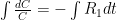
Surely they don’t serious use the sum of five or six exponentials, Willis. Nobody could be that dumb. The correct ordinary differential equation for CO_2 concentration , one that assumes no sources and that the sinks are simple linear sinks that will continue to scavenge CO_2 until it is all gone (so that the “equilibrium concentration” in the absence of sources is zero (neither is true, but it is pretty easy to write a better ODE) is:

 is the rate at which the ocean takes up CO_2. Left to its own devices and with only an oceanic sink, we would have:


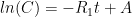
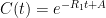
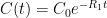
 is the constant of integration. I mean, this is first year calculus. I do this in my sleep. The inverse of $R_1$ is the exponential decay constant, the time required for the original CO_2 level to decay to
  of its original value (for any original value
  ). If there are two processes running in parallel, the rate for each is independent — if (say) trees remove CO_2 at rate $R_2$, that process doesn’t know anything about the existence of oceans and vice versa, and both remove CO_2 at a rate proportional to the concentration in the actual atmosphere that runs over the sea surface or leaf surface respectively. The same diffusion that causes CO_2 to have the same concentration from the top of the atmosphere to the bottom causes it to have the same concentration over the oceans or over the forests, certainly to within a hair. So both running together result in:
 , the exponential time constant is 1/5 of what it would be for one of them alone. This is not rocket science.

 ,
,  :
:
Interpretation: Since CO_2 doesn’t come with a label, EACH process of removal is independent and stochastic and depends only on the net atmospheric CO_2 concentration. Suppose
where
If (say) trees and the ocean both remove CO_2 at the same independent rate, the two together remove it at twice the rate of either alone, so that the exponential time constant is 1/2 what it would have been for either alone. If there are five such independent sinks (where by independent I mean independent chemical processes), all with equal rate constants
This is completely, horribly different from what you describe above. To put it bluntly:
Compare this when
(correct) versus
(incorrect). The latter has exactly twice the correct decay time, and makes no physical sense whatsoever given a global pool of CO_2 without a label. The person that put together such a model for CO_2 — if your description is correct — is a complete and total idiot.
Note that this would not be the case if one were looking at two different processes that operated on two different molecular species. If one had one process that removed CO_2 and one that removed O_3, then the rate at which one lowered the “total concentration of CO_2 + O_3” would be a sum of independent exponentials, because each would act only on the partial pressure/concentration of the one species. However, using a sum of exponentials for independent chemical pathways depleting a shared common resource is simply wrong. Wrong in a way that makes me very seriously doubt the mathematical competence of whoever wrote it. Really, really wrong. Failing introductory calculus wrong. Wrong, wrong, wrong.
(Dear Anthony or moderator — I PRAY that I got all of the latex above right, but it is impossible to change if I didn’t. Please try to fix it for me if it looks bizarre.)
rgb
Nullius in Verba says:
May 6, 2012 at 11:19 am (Edit)
My thanks for your explanation. That was my first thought too, Nullius. But for it to work that way, we have to assume that the sinks become “full”, just like your tank “B” gets full, and thus everything must go to tank “C”.
However, since the various CO2 sinks have continued to operate year after year, and they show no sign of becoming saturated, that’s clearly not the case.
So what we have is more like a tank “A” full of water. It has two pipes coming out the bottom, a large pipe and a narrow pipe.
Now, the flow out of the pipe is a function of the depth of water in the tank, so we get exponential decay, just as with CO2.
But what they are claiming is that not all of the water runs out of the big pipe, only a certain percentage. And after that percentage has run out, the remaining percentage only drains out of the small pipe, over a very long time … and that is the part that seems physically impossible to me.
I’ve searched high and low for the answer to this question, and have found nothing.
w.
What about rain water, which, in its passage through the air dissolves many of the soluble gases e.g. CO2 present in the atmosphere, and which as part of ‘river waters’ eventually makes its way into the oceans?
River and Rain Chemistry
Book: “Biogeochemistry of Inland Waters” – Dissolved Gases
.
“The IPCC, using the Bern Model, says that the e-folding time ranges from 50 to 200 years.”
**********************
Strikes me as a pretty wide ranging estimate. More like a ‘WAG’.
I file this Bern Model under “more BAF (Bovine Academic Flatulence)”.
The physiology of scuba diving divides body tissues into different categories, with different “half-lives”, or nitrogen abosrption rates. Some tissues absorb, and release Nitrogen rapidly, others more slowly; they are given different diffusion coefficients.
Nitrogen absorbed in your tissues in diving is the cause of the bends.
Maybe the Bern Conspiracy is thinking that some absorption mechanisms operate at different rates others. How fast do forests absorb CO2 compared to oceans? etc. Perhaps that is what they are thinking.
mfo says:
May 6, 2012 at 11:19 am
mfo, take a re-read of my appendix above. The author of the hockeyschtick article is conflating the residence time and the e-folding time. As a result, he sees one person saying four years or so for residence time, and another person saying 50 to 200 years for e-folding time, and thinks that there is a contradiction. In fact, they are talking about two totally separate and distinct measurements, residence time and e-folding time.
w.
Willis Eschenbach says:
May 6, 2012 at 12:07 pm
“What I don’t get is what causes the fast sequestration processes to stop sequestering, and to not sequester anything for the majority of the 371.6 years … and your explanation doesn’t explain that.”
The best I can tell you is what I stated:”It has to do with the frequency of CO2 molecules coming into contact with absorbing reservoirs (a.k.a. sinks). If the atmospheric concentration is large, then molecules are snatched from the air frequently. If it is smaller, then it is more likely for an individual molecule to just bob and weave around in the atmosphere for a long time without coming into contact with the surface.” The link I gave explains it from a mathematical viewpoint.
rgbatduke says:
May 6, 2012 at 12:12 pm
“The correct ordinary differential equation…”
It’s a PDE, not an ODE. See comment at May 6, 2012 at 11:51 am.
About 1/2 of the annual human emission are absorbed each year. If they weren’t the growth in CO2 as a % of total would be growing, which it isn’t.
Assuming an exponential rate of uptake, we have a series something like this:
1/2 = 1/4 + 1/8 + /16 + 1/32 ….
With each year absorbing 1/2 of the residual of the previous, to match the rate of the total.
ie: R = R^2 + R^3 + R^4 … R^n , where 0 < R infinity.
What this means is that tau is 2 years. 1/4 + 1/8 = 0.25 + 0.125.= 0.375 = approx 1/e
The mathematical and physical ability of climate scientists appears to be very poor.
The worst case is the assumption by Houghton in 1986 that a gas in Local Thermodynamic Equilibrium is a black body. This in turn implies that the Earth’s surface, in radiative equilibrium, is also a black body, hence the 2009 Trenberth et. al. energy budget claiming 396 W/m^2 IR radiation from the earth when the reality is presumably 63 of which 23 is absorbed by the atmosphere.
The source of this humongous mistake is here: http://books.google.co.uk/books?id=K9wGHim2DXwC&pg=PA11&lpg=PA11&dq=houghton+schwarzschild&source=bl&ots=uf0NxopE_H&sig=8vlpyQINiMyH-IpQrWJF1w21LQU&hl=en&sa=X&ei=6Z2mT7XyO-Od0AWX3LGTBA&ved=0CGMQ6AEwBA#v=onepage&q&f=false
Here is the [good] Wiki write-up: http://en.wikipedia.org/wiki/Thermodynamic_equilibrium
‘In a radiating gas, the photons being emitted and absorbed by the gas need not be in thermodynamic equilibrium with each other or with the massive particles of the gas in order for LTE to exist….. If energies of the molecules located near a given point are observed, they will be distributed according to the Maxwell-Boltzmann distribution for a certain temperature.’
So, the IR absorption in the atmosphere has been exaggerated by 15.5 times. The carbon sequestration part is no surprise; these people are totally out of their depth so haven’t fixed the 4 major scientific errors in the models.
And then they argue that because they measure ‘back radiation’ by pyrgeometers, it’s real They have even cocked this up: a radiometer has a shield behind the detector to stop radiation from the other direction hitting the sensor assembly. So, assuming zero temperature gradient, the signal they measure is an artefact of the instrument because in real life it’s zero. What is measures is temperature convolved with emissivity, and so long as the radiometer points down the temperature gradient, that imaginary radiation cannot do thermodynamic work!
This subject is really the limit of cooperative failure to do science properly. Even the Nobel prize winner has made a Big Mistake!
I’m not sure of the significance of the e-folding time. I presume it must be related to the rate at which a particular sink absorbs CO2, in which case why not use the absorption time? As for the partitions, I just don’t get it. Surely there must be a logical explanation in the text for the various percentages listed.
ferd berple says:
May 6, 2012 at 12:25 pm
“About 1/2 of the annual human emission are absorbed each year.”
In the IPCC framework, that 1/2 dissolves rapidly into the oceans. So, if you include both the oceans and the atmosphere in your modeling, there is no rapid net sequestration.
I agree with the IPCC on the former. But, I do not agree with them that the collective oceans and atmosphere take a long time to send the CO2 to at least semi-permanent sinks.
Bart says:
May 6, 2012 at 12:21 pm
No, the link you gave explains simple exponential decay from a mathematical viewpoint, which tells us nothing about the Bern model.
w.
Willis said: What I don’t get is what causes the fast sequestration processes to stop sequestering, and to not sequester anything for the majority of the 371.6 years … and your explanation doesn’t explain that.
================================
Either there are five different types of CO2…..or CO2 is not well mixed at all……or each “tau” has a low threshold cut off point
The only things that can have a low threshold cutoff point are biology
Cos the other sinks are fully saturated, or already absorbing all they can, so they leave the rest behind for the other longer sinks – then they can claim the natural sinks are saturated and we are evil despite it making no sense. Its all based on the assumption that before 1850 co2 levels were constant and everything lived in a perfect state of equilibirum just on the very the systems absorbtion capacity. Ahhh the world of climate science!
I must step away, so apologies if anyone has a question or challenge to anything I have written. Will check the thread later.
All I’ve got time for today is: Here we go again …
Welcome to the ‘troop’ which denies the measurable EM-nature of bipolar gaseous molecules, e.g. is studied in the field of IR Spectroscopy.
.
The rate of each individual sink is meaningless. What is important is that the total increase each year remains approximately 1/2 of annual emissions. Everything else is simply the good looking girls the magician uses to distract the audience from the sleight of hand.
As Willis points out, the thermos cannot know if the contents are hot or cold. Similarly, the sinks cannot know how long the CO2 has been in the atmosphere, so you cannot have differential rates depending on the age of the CO2 in the atmosphere.
1/2 the increased CO2 is absorbed each year. therefore 1/2 the residue must also be absorbed year to year. The sinks cannot tell if it is new CO2 or old CO2.
What are the mechanisms for removing CO2 from the atmosphere?
1. Asorbsion at the surface of seas and lakes
2, Absorbsion by plants through their leaves
3, Washed out by rain.
Any others?
What is the split in magnitude between these methods because I’d expect some sort of equilibrium for each of 1 & 2 whereas 3 seems to be one way.
Every year this lady named Mother Nature adds a whole lot of CO2 to the atmosphere, and every year she takes out a whole lot. The amount she adds in a given year is only loosely correlated with the amount she takes out, if at all. Year after year we add a little more CO2 to the atmosphere, still only around 4% of the average amount MN does. There is no basis for contending that the amount we add is responsible for what may or may not be an increased concentration with respect to recent history. All we know is that CO2 frozen in ice averages around 280 ppm, but this is definitely an average value as the ice can take hundreds of years to seal off. The only numbers in this entire discussion that have a basis in fact are 220 gT in and out, and an average four year residence time. All else is speculation/conjecture/WAG.
Occam’s Razor rules as always.
Bart says:
May 6, 2012 at 12:32 pm
In the IPCC framework, that 1/2 dissolves rapidly into the oceans.
Nonsense. The oceans cannot tell if that 1/2 comes from this year or last year. If the oceans rapidly absorb 1/2 of the CO2 produced this year, then they must also rapidly absorb 1/2 the remaining CO2 from last year in this year. And so on and so on, for each of the past years.
The ocean cannot tell when the CO2 was produced, so it cannot have a different rate for this years CO2 as compared to CO2 remaining from any other year.
rgbatduke says:
May 6, 2012 at 12:12 pm
Thanks, Robert, your contributions are always welcome. Unfortunately, that is exactly what they do, with the additional (and to my mind completely non-physical) restriction that each of the exponential decays only applies to a certain percentage of the atmospheric CO2. Take a look at the link I gave above, it lays out the math.
Your derivation above is the same one that I use for the normal addition of exponential decays. I collapse them all into the equivalent single decay with the appropriate time constant tau.
But they say that’s not happening. They say each decay operates only and solely on a given percentage of the CO2 … that’s the part that I can’t understand, the part that seems physically impossible.
w.