There’s a saying, “timing is everything”. After reading this, I think it is more true than ever. In other news. Paul Vaughn is giving Bob Tisdale serious competition in the contest over who can fit the most graphs into a single blog post. ☺ There is a helpful glossary of symbols and abbreviation at the end of this post that readers would benefit from reading before the essay. A PDF version is also available via link at the end of the article. – Anthony
Guest post by Paul L. Vaughan, M.Sc.
Lack of widespread awareness of the spatiotemporal nature of interannual terrestrial oscillations is perhaps the most paralyzing bottleneck in the climate discussion.
North Pacific Pivot
Elegant factor analyses by Trenberth, Stepaniak, & Smith (2005) concisely chart the limits of linear climate exploration, providing strong clues that the North Pacific is a globally pivotal intersection.

D – T = -SOI (an index of El Nino / La Nina – details below in “Data & Symbols” section)
WUWT readers are well-acquainted with Tsonis, Swanson, & Kravtsov (2007). Recently Wyatt, Kravtsov, & Tsonis (2011b) shared the following on Dr. Pielke Senior’s blog:
“PNA participates in all synchronizations.”
Orientation for ENSO- & PDO-centric readers:

Complex Correlation
Simple linear correlation can do a part-way decent job of summarizing the preceding intrabasin relations, but properties of interbasin & interhemispheric multiscale spatiotemporal relations clarify the need for complex summaries. For example:

Limitations of linear methods are emphasized by Maraun & Kurths (2005). A mainstream audience might not appreciate their beautifully concise section 3 primer, but there’s a simple way to look at interannual spatiotemporal phasing.

The ~2.37 year signal which is so prominent in the equatorial stratosphere is also easily detected in the troposphere, but there’s clearly “something else” contributing to interannual tropospheric variation.

Note that when iNPI’ doesn’t “go with” iAAM & iLOD, it “goes against” them, much like a switch that is either “off” or “on”. Specialists like Maraun & Kurths might speak of coherence and illustrate the nonrandom distribution of phase differences.
Multiscale complex correlation (for example using adjacent derivative based complex empirical wavelet embeddings) can measure complex nonstationary relations where simple linear correlation fails catastrophically. Naive investigators unknowingly encounter Simpson’s Paradox by falsely assuming independence and blindly running linear factor analyses (such as PCA, EOF, & SSA) without performing the right diagnostics.
Northern Hemisphere Inter-Basin Interannual Coherence
Nonrandom phase relations explored by Schwing, Jiang, & Mendelssohn (2003):


Interannual Solar-Terrestrial Phase-Relations
Terrestrial phase relations with interannual [not to be confused with decadal] rates of change of solar variables, including solar wind speed (iV’), are nonrandom:


Inter-Hemispheric Interannual Phase-Relations
For those wondering how AAO & SAM fit in:


Global Synchronicity
Synchronicity’s the norm. Orientation, configuration, amplitude, & extent of globally constrained & coupled jets & gyres are pressured while network monitoring remains stationary. Regional temporal phase summaries are intermittently flipped by the stationary spatial geometry of monitoring networks in the turbulent global context.

Note particularly (in the last 2 graphs) the strong & stable interannual synchronicity of northern annular, southern annular, & global modes for the decade beginning ~1988. The commencement of the pattern coincides with concurrent abrupt changes in Arctic ice flow (e.g. Rigor & Wallace (2004) Figure 3) and European temperature (e.g. Courtillot (2010)).
Local Connection
Here’s how NPI relates to minimum temperatures at my local weather station:


Concluding Speculation
Terrestrial geostrophic balance is affected by the concert of changes in:
a) interannual (not to be confused with decadal) solar variations.
b) decadal amplitude of semi-annual Earth rotation variations – [see Vaughan (2011) & links therein].
c) solar cycle length – [see links in Vaughan (2011)].
Nipping Potential Misunderstandings in the Bud
“So you’re claiming the North Pacific controls global climate?”
No.
Why do I hear the same places mentioned every rush hour on the traffic report? Bottlenecks are easy places to detect changes in pressure & flow (whether global &/or locally intersecting), even using the simplest methods. Methods such as those suggested by Schwing, Jiang, & Mendelssohn (2003); Maraun & Kurths (2005); and Tsonis, Swanson, & Kravtsov (2007) help expand our vision towards the rest of the network. We have a lot of work to do (both exploratory & methodological).
Further Reading
Everything written by Tomas Milanovic at Dr. Judith Curry’s blog Climate Etc.
Vaughan, P.L. (2011). Solar, terrestrial, & lunisolar components of rate of change of length of day.
Referenced Above
Courtillot, V. (Dec. 2010). YouTube Video (~30min): Berlin Conference Presentation.
http://www.youtube.com/watch?v=IG_7zK8ODGA
Maraun, D.; & Kurths, J. (2005). Epochs of phase coherence between El Nino-Southern Oscillation and Indian monsoon. Geophysical Research Letters 32, L15709. doi10.1029-2005GL023225.
http://www.cru.uea.ac.uk/~douglas/papers/maraun05a.pdf
Rigor, I.; & Wallace, J.M. (2004). Variations in the age of Arctic sea-ice and summer sea-ice extent. Geophysical Research Letters 31. doi: 10.1029/2004GL019492.
http://iabp.apl.washington.edu/research_seaiceageextent.html
Schwing, F.B.; Jiang, J.; & Mendelssohn, R. (2003). Coherency of multi-scale abrupt changes between the NAO, NPI, and PDO. Geophysical Research Letters 30(7), 1406. doi:10.1029/2002GL016535.
Trenberth, K.E.; Stepaniak, D.P.; & Smith, L. (2005). Interannual variability of patterns of atmospheric mass distribution. Journal of Climate 18, 2812-2825.
http://www.cgd.ucar.edu/cas/Trenberth/trenberth.papers/massEteleconnJC.pdf
Tsonis, A.A.; Swanson, K.; & Kravtsov, S. (2007). A new dynamical mechanism for major climate shifts. Geophysical Research Letters 34, L13705.
http://www.nosams.whoi.edu/PDFs/papers/tsonis-grl_newtheoryforclimateshifts.pdf
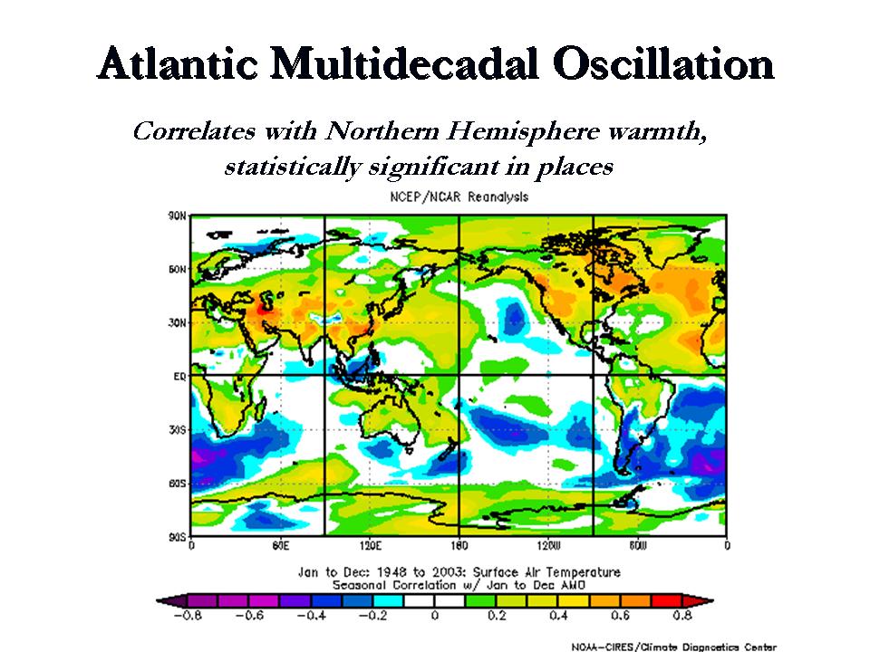
Wyatt, M.G.; Kravtsov, S.; & Tsonis, A.A. (2011). Atlantic Multidecadal Oscillation and Northern Hemisphere’s climate variability. Climate Dynamics. doi: 10.1007/s00382-011-1071-8.
Since (to my knowledge) there’s not yet a free version, see the conference poster and the guest post at Dr. R.A. Pielke Senior’s blog for the general idea:
a) Wyatt, M.G.; Kravtsov, S.; & Tsonis, A.A. (2011a). Poster: Atlantic Multidecadal Oscillation and Northern Hemisphere’s climate variability.
https://pantherfile.uwm.edu/kravtsov/www/downloads/WKT_poster.pdf
b) Wyatt, M.G.; Kravtsov, S.; & Tsonis, A.A. (2011b). Blog: Atlantic Multidecadal Oscillation and Northern Hemisphere’s climate variability.
Important Note: While Wyatt, Kravtsov, & Tsonis (2011) are likely to stimulate a lot more discussion once a free version of their paper becomes available, it needs to be pointed out assertively & clearly that the cross-correlation approach, while informative, is patently insufficient for determining the full nature of terrestrial spatiotemporal phase relations.
Appendices
In the appendices that follow, attention is concisely drawn to key items that are consistently underappreciated in climate discussions.
Appendix A: Spatial Influence on Phase – Important
Nonrandom phase relations demand careful focus on the spatial dimension. Temporal evolution isn’t the only thing driving apparent phase.
If features grow, shrink, rotate, change shape, reflect, or move relative to the stationary windows in which they are measured, phase is affected.


The effect on summaries is plain & simple. (Anyone previously puzzled by “integration across spatiotemporal harmonics” might now get the general idea.)
Appendix B: Reversals in Temperature-Precipitation Relations
Blink between winter & summer panels of Figure 6:
Trenberth, K.E. (2011). Changes in precipitation with climate change. Climate Research 47, 123-138. doi: 10.3354/cr00953.
http://www.int-res.com/articles/cr_oa/c047p123.pdf
Temperature-precipitation relations are a function of absolutes, not anomalies. This is fundamentally important.
Insight from my local (ABC) example:


Appendix C: Global Distribution of Continental-Maritime Contrast
High-amplitude regional variance leverages global summaries, but multidecadal variations often draw misguidedly narrowed focus to the North Atlantic Ocean when it is the global distribution of continental-maritime contrast (in relation to flow patterns) that should be attracting the attention. Noting the position of the relatively small North Atlantic in this broader context, carefully compare:
1. http://icecap.us/images/uploads/AMOTEMPS.jpg
2. Figure 10 here:
Carvalho, L.M.V.; Tsonis, A.A.; Jones, C.; Rocha, H.R.; & Polito, P.S. (2007). Anti-persistence in the global temperature anomaly field. Nonlinear Processes in Geophysics 14, 723-733.
http://www.icess.ucsb.edu/gem/papers/npg-14-723-2007.pdf
Data & Symbols
‘ indicates rate of change
[ ] indicates time-integration
AAM = Atmospheric Angular Momentum
AAO = AntArctic Oscillation
ABC = Agassiz, British Columbia (west coast of Canada near USA border)
AO = Arctic Oscillation
COWL = Cold Ocean, Warm Land index
D-T = -SOI = – Southern Oscillation Index = pressure difference between Darwin & Tahiti (an indicator of El Nino / La Nina cycling)
ENSO = El Nino / Southern Oscillation
i = interannual
LOD = Length Of Day
NAO = North Atlantic Oscillation
NPI = North Pacific Index
PDO = Pacific Decadal Oscillation
PNA = Pacific North America index
PPT = PreciPiTation
QBO = QuasiBiennial Oscillation
SAM = Southern Annular Mode
SOI = Southern Oscillation Index
T = Temperature (°C)
V = solar wind speed
x = extreme
Data links available upon request.
Acknowledgements
Sincere thanks to Anthony Watts, the WUWT Moderation Team, readers, and all those who make valuable contributions towards a deeper understanding of nature.
==========================================================
PDF Version of this essay available here Vaughan, P.L. (2011). Interannual Terrestrial Oscillations (375KB)
From my years of electronics communications work modulating and then demodulating signals that have been transmitted over a radio frequency carrier method, I can see ways the overall long term signals in the weather and climate data could be understood.
If the longest wave pattern indicative of a composite wave pattern is used as the key for the demodulation of the packets of individual periods of oscillation patterns, then the over lapping of several periods of these patterns should give an indication of the reproducibility of the original signals.
The inner planets and the outer planets have their own separate periods of harmonic oscillation as a result of billions of years of gravitational, tidal and electromagnetic interactions that are in a resonate pattern, the inner planets have a beat frequency of about 6558 day period with the outer planets settled into a period of somewhere between 172 and 179 years.
Most of the cyclic patterns seen in the above graphs are a result of the shorter term periods of interactions of both the inner planets and the outer planets beating together and generating these short term affects in the global circulation patterns.
As RC Saumarez says:
May 16, 2011 at 10:14 am
“We only have one climate record and therefore we cannot use an ensemble approach without segmentation of the data and thus limit the minimum observable frequency.”
To solve this problem I looked at three patterns of the 6558 day period, overlaid them at the daily weather data level, and plotted the resultant combined signal for Precipitation, and temperature patterns for the USA, extended that cyclic interpenetration for a six year period, and plotted out maps to show the repeating reoccurring patterns in the global circulation, as a ( 6 year long stretch, we are now ~40 months into the posted 6 years long) forecast for part of the current repeat of the 6558 day long cycle.
The precipitation patterns repeat well enough to show the locations of the repeat of the 1974 tornado out break we had this spring, and will also show the repeat of the severe flooding in Australia. The problem with this forecast technique is the outer planet ~172/179 year pattern is out of phase with the inner planet harmonics so it needs to be compensated for as well.
The best method I have come up with so far would be to plot the data excursions from the expected past 6558 day patterns, by looking at the 5 to 10 day long disruptions caused by the current 6558 day period heliocentric (or Synod) conjunctions, as the corrective algorithms to adjust the inner planet patterns for the effects of the outer planet modulations.
The Earth has a synod conjunction with each of the four major gas planets with a little over a year between impulses, (~+2 days for Neptune, ~+4 days for Uranus, ~+13 days for Saturn, ~+34 days for Jupiter) these past almost annual periods could be segmented and applied into the composite forecast as an adjustment algorithm to further enhance the pattern match, to increase the accuracy (~85%) of the inner planet 6558 day pattern to closer to 95% with the addition of the compensation for the outer planet interactive influences.
I am in the process of rewriting the map making software to fine tune the resultant process to get a better repeatability of the temperatures as well. With the next posting of updated several year long series of forecast maps I will be including the areas of Alaska, Canada, and Australia (with enough hind cast [+6 months] to show how well it did with the flooding there). I will be adding a fourth cycle going back another 6558 day period to use the additional analog year starting in ~1938 for 2011.
If any of the readers here have helpful suggestions on how this could be better accomplished, I would like to hear from them.
Paul
My brain has tried to work out what your article is about and what it has come up with is that there are many things affecting the climate and to try and remedy one of them is a waste of time.
PS glad you can spell Vaughan correctly.
Paul says:
“The interannual filter used simply contrasts years with immediately-adjacent years for each variable. Amplitude is normalized to facilitate visualization.”
Now it starts to make sense even though I have not got the first clue as to how the data is generated.
My take:
Mathematical techniques to check associations can get us only so far. Even if the association is perfect we have to know why, i.e. what the driver is. I can help in that respect and answer the question that Paul poses in this way: Erl, I’m wondering if you are seeing some connection between this [ http://wattsupwiththat.files.wordpress.com/2011/05/vaughn_npp_image8.png ] and your work on polar voritices & geomagnetic Dst index?”
Yes, I can. The polar circulations couple the troposphere and the stratosphere. In the southern hemisphere the result is a zone of very low surface atmsopheric pressure at latitude 60-70 degrees south due to the descent of ozone into the troposphere, the resultant warming and reduced weight of the atmospheric column. The ‘annular ring’ of lower surface atmsopheric pressure is amost complete (ring like) but it is broken by the influence of the landmasses of the southern hemisphere. In the southern hemsiphere the flux in ozone into the tropsophere is continuous throughout the year but the background levels of ozone are comparatively much lighter than in the northern hemsiphere and the influence on cloud cover (as inferred from change in sea surface temperature) is perceptible only at higher latitudes.
In the northern hemsiphere ozone descent into the troposphere occurs in the main in northern winter because it is at this time that the troposphere and stratosphere become a strongly coupled circulation. The coupling depends upon the estabishment of a regime of air temperature declining continuously with increasing elevation into the mid-stratosphere, favouring convection, as it does in the troposphere.
Because the Arctic stratosphere has relatively high levels of ozone (relatively unaffected by coupling in summer) the effect on cloud cover (as inferred via change in sea surface temperature when compared with flux in surface pressure in the main zones of ozone descent) is much more dramatic, more obviously synchronised and coherent than it is in the southern hemisphere and the influence extends as far as the mid latitudes of the southern hemisphere.
Proving all this in a satisfying way is not something that can be done in this post but I refer readers to http://www.happs.com.au/images/stories/PDFarticles/TheCommonSenseOfClimateChange.pdf
In that work I also deal with the connection between geomagnetic indices and surface pressure and the way in which the polar votices affect backround levels of ozone in the polar stratosphere.
Now, I want to get the the main thrust of Pauls post that suggests that the North Pacific is pivotal in the process of short and long term climate change.
The pattern of descent of ozone into the troposphere in the northern hemsiphere is affected by the distribution of land and sea in just the same way as in the southern hemisphere. But there is more land and less sea. The upshot is one zone of descent in the north Pacific and another across the north Atlantic.
What I am referring to here is what has been described by Baldwin, Dunkerton and others only since the turn of the century as the northern and the southern annular modes, recognized as associated with interannual climate variability. But so far ‘we know not how’. In other words, the maths points to the association, the spato-temporal aspects are well described but the understanding of process is as yet so slight as to be insignificant.
Climate change is driven from the poles. The most obvious links are via the NAM (Northern Annular Mode), that is synchronous with the Arctic Oscillation. It has long been recognized that there is a close relationship between solar indices and the Arctic Oscillation in northern winter months. In my work I reference Palamara in that respect.
The weakness of all correlative work comes down to lack of understanding of process. I suggest that this situation will change as we build on the current understanding of the NAM and the SAM and understand the importance of convection in the polar atmsophere and it’s importance in driving stratospheric ozone levels and tropospheric cloud cover.
CommieBob’s video link is highly explanatory.
The simple pendulum experiment shows that oscillators of any type can show all sorts of correlations that are purely artifacts of the point of view. Look at the pendulum experiment from the side and you simply see 16 pendulums swing side by side at different frequencies. If they had panned around the platform at other angles other apparent correlations or patterns would have appeared.
It’s related to Steveta_uk’s tick-tock cycle generated by two watches. Or the beautfiful Moire’ patterns you can see through layers of silk. The Moire’ patterns come from minute guage and thread diameter variations in the silk and the angle of the lighting. Neither one contains any information except about the frequencies involved. Theoretically, you could take the period of the tick-tocks and calculate the exact relative frequency of each watch. You could model the spacial Moire’ patterns and estimate the guage and diameter variations of the sllk. But the patterns themselves don’t carry any information about the cause of the oscillation or pattrern
This paper has the same problem. Any kind of correlations between oscillators don’t tell us anything about the mechanism of what is actually going on. In order to get that you would need an accurate model of say the Pacific Decadel Oscillation- where the ocean flows, temperatures, winds, etc., are known and then extend it to include how the various ocean basins interact. Not to take shots at Leif Svalgaard, but the correlations don’t really even show that the items are interdependent. To do that you would have to show how they are connected, which is more than mere correlation.
George E. Smith says:
I saw the video first on http://www.boingboing.net . Here’s a quote.
In other words, each pendulum has a subharmonic whose period is one minute.
commieBob says:
May 16, 2011 at 6:06 pm
From the shortest pendulum to the longest, each pendulum is one swing per minute less than the one before it. The effect is a hypnotic dance that repeats every 60 seconds.
But which does not demonstrate synchronization at all, as there is no coupling between the pendulums. The dance is totally artificial and contrived.
Richard Holle
I look forward to reading your work, particularly releating to Australia.
Paul Vaughan
I realise that the following will be hurtful, BUT:
I suggest that you give your paper to someone who is expert in communication.
It needs to be completely re-written, showing exactly what you are criticising (not just saying that there are many examples) and explaining how and why your method is superior.
But please, do not attempt this task yourself.
Leif, I [not you] decide what will convince me that iNPI’ & other i-waves are independent of iV’. As indicated above, I’m willing to be convinced, but I’m skeptical that anyone can produce a convincing argument.
As for the other “misunderstanding”:
You know very well the following:
“Let X1, X2, X3, … ~i.i.d.”
You also know very well the demands for some kind of formal statistical inference in formal pubs.
Linear methods alone aren’t sufficient for inference on these variables. There are plenty of methods that COULD be developed that might lead to far more meaningful p-values and confidence intervals. One sees the pioneering going on, but it’s not all the way there yet.
A merger of something like Maraun & Kurths hybridized with cross-wavelet methods and VEOF is one suggestion I’ve pitched to a local expert on nonlinear factor analysis. Unfortunately, he’s retiring. Currently I lack the resources to pursue the project independently, but I’ve developed a prototype.
After developing the prototype, I decided the audience here would not understand the algorithm output — hence the decision to post simple graphs and see if folks’ intuition is enough to see what the algorithm sees. The comments provide valuable feedback. I find it particularly interesting that most of those sufficiently motivated to comment appear more concerned with formal cosmetics than informal climate discussion.
Erl, thanks for your interesting comments.
Thanks to all who have commented.
I fully expected serious misunderstandings & vicious feedback on this informal article.
I firmly retain my opening assertion:
“Lack of widespread awareness of the spatiotemporal nature of interannual terrestrial oscillations is perhaps the most paralyzing bottleneck in the climate discussion.”
Leif Svalgaard’s first paragraph in his first post and the comment from John Syfret assured me: Mission accomplished on the Pareto Principle with anticipated & entirely acceptable collateral damage.
Best Regards to All.
Paul Vaughan says:
May 16, 2011 at 8:25 pm
Leif, I [not you] decide what will convince me that iNPI’ & other i-waves are independent of iV’. As indicated above, I’m willing to be convinced, but I’m skeptical that anyone can produce a convincing argument.
As Richard Feynman once remarked, the easiest one to fool is oneself. You have not even described what the relationship is. Suppose that the solar wind speed depends on the day of the year. What would that do to the ‘relationship’? with the seasons being a confounding variable…
This comment is addressed to all those who have criticised this post on the basis that correlation is fortuitious, and unrelated to causation. It is also addresssed to those who find the presentation obscure and those who maintain that ‘wiggle matching’ is unlikely to bear fruit.
The task of identifying the cause of climatic variations that are sometimes described as ‘natural variations’ involves demonstrating a plausible mechanical link between variables that is consistent. What we have in this post is simply a demonstration of the consistency, or lack thereof in the links between certain indices that are known to relate to variations in temperature and rainfall in some locations on the globe.
If a pattern of variation is consistent for a period of time and becomes inconsistent it possibly represents the waxng and waning influence of second or third drivers. For example, there are two poles and the influence of these poles changes over time.
It is easy to criticise the work because of what it is not. The work makes no attempt to describe modes of causation although it is suggested that iV, the variation in the solar wind could be involved. As I intimated above, that suggestion is not novel, so far as it relates to the northern annular mode, also described as the Arctic Oscillation. But, here it is shown that variation in iV relates to more indices. That’s progress. No work could survive scrutiny if it could be criticised on the basis that it does not provide a complete picture of the world. So, much of the criticism here is irrelevant.
Matching the wiggles is the first observational task. A mathematical technique that enables one to identify the degree of symmetry is valuable.
The second task is to explain why the wiggles match. It would be nice to have the two together but it is not always possible.
Leif does not appear to contradict the proposition that the wiggles match in a way that suggests they could be related. That is progress indeed.
Others will suggest why the wiggles relate as they do and their work is made easier to the extent that the degree to which variables move together has been identified.
Then there is the sort of criticism offered by Ausie Dan, which is just posturing, egotisitical, and hurtful. No place for that at all. A really cheap shot. A stone thrower getting into the act.
I look in vain for the person who asks the simple question: Why is it so? When that question is asked the real discussion begins.
Leif, whether relationships are physical or not, they are still of interest to someone who catalogs them. Awareness of confounding is preferable to ignorance of it. I understand your concern that some innocents will misunderstand. I also acknowledge that physicists define “relationship” differently than do statisticians.
Eloquent words Erl (erlhapp May 16, 2011 at 9:43 pm).
Fyi: The relationship with iNPI’ is much tighter & much more systematic than with iAO’ & iNAO’ (or iNAM’ if you prefer).
Thanks Paul,
Info at http://www.cgd.ucar.edu/cas/jhurrell/indices.info.html#np is useful.
On solar and terrestrial links
http://www.vukcevic.talktalk.net/CD.htm
with more details to follow.
Leif Svalgaard says:
May 16, 2011 at 9:15 pm
You have not even described what the relationship is. Suppose that the solar wind speed depends on the day of the year. What would that do to the ‘relationship’? with the seasons being a confounding variable…
Paul, you ducked this question.
erlhapp says:
May 16, 2011 at 9:43 pm
The work makes no attempt to describe modes of causation although it is suggested that iV, the variation in the solar wind could be involved. […]
Matching the wiggles is the first observational task. A mathematical technique that enables one to identify the degree of symmetry is valuable.
Except that no attempt was made to quantify the degree of wiggle matches.
Leif does not appear to contradict the proposition that the wiggles match in a way that suggests they could be related. That is progress indeed.
Let me try to go behind ‘appearance’. I don’t think the wiggles match enough to be of interest. Since Paul ducks quantifying the claimed match, no progress seems possible.
Paul Vaughan says:
May 16, 2011 at 10:26 pm
I understand your concern that some innocents will misunderstand.
We are all ‘innocents’ in this game, except the guilty ones.
I also acknowledge that physicists define “relationship” differently than do statisticians.
There is a strong relationship between shoe size and reading ability among school children. A statistician concludes that bigger feet helps the child to learn to read. As I said, all the other graphs [apart from the one with iV] presented were just correlating climate with climate so are not of any relevance or interest. The iV ‘relation’ is not quantified and the solar wind speed time series does not seem to have any spatial aspect to it to merit the notion of ‘spatiotemporal’.
So, it would perhaps be of interest to examine the iV graph in detail.
1) Where does the solar wind data come from?
2) How is the data smoothed? precisely, how is the techniques of section 3 of Maraun & Kurths applied to the data?
3) Can you quantify the non-randomness?
4) Address the confounding aspect with solar wind speed depending on time of year
Leif Svalgaard falsely asserted (May 17, 2011 at 4:08 am):
“Except that no attempt was made to quantify the degree of wiggle matches.”
Correction to the statement:
Multiscale complex correlation has not been presented in this article, but it has been measured by 2 different methods.
The annual & semi-annual signals (phase-locked to the terrestrial year) are on my radar, as are the dependence of your V reconstruction on space and the skewed distribution of your proxy.
–
Leif Svalgaard also falsely asserted (May 17, 2011 at 4:08 am):
“A statistician concludes that bigger feet helps the child to learn to read.”
Here you’re just having fun playing to the audience.
Some stats profs go to a fair amount of trouble cautioning their students about how to write conclusions that are technically correct. The most common error is failure to acknowledge conditional dependence of interpretations on null hypothesis model assumptions. In your example it would be technically correct to note a relationship between shoe size & reading skill. In an introductory level course, one might take the opportunity to reinforce lessons about confounding & lurking variables.
—
I developed my own methods independently well before I ever read Maraun & Kurths (2005). When I found the paper (& its section 3 in particular), it became a convenient link. Same comments would apply to Schwing, Jiang, & Mendelssohn (2003) [except that the free version of their paper has disappeared from the web].
I explained the filtering above (in response to a question from Erl). I can add that the normalization is based on the maximum absolute deviation.
Pursuing p-values & confidence intervals would be premature at this stage. More thorough data exploration is prerequisite to sensible statistical inference (contrary to dominant mainstream pressures that ignore Simpson’s Paradox).
vukcevic, I look forward to reading the article you’re assembling.
NPI:
http://www.cgd.ucar.edu/cas/jhurrell/Data/npindex.mon.asc
Leif Svalgaard says:
May 16, 2011 at 7:48 pm
Almost every waveform I have ever looked at was totally artificial and contrived. 😉
It doesn’t matter if the pendulums are actually coupled or not. If we were to actually synchronize them with a clock pulse whose period was one minute, their oscillations would look the same (except they might not be damped).
Paul Vaughan says:
May 17, 2011 at 7:35 am
…………….
Paul
Some scientists often get into ‘gainsay’ arguments to the extent where further exchange of views is counter productive.
What I will be presenting is a natural ‘down to Earth’ likely cause for the climate change based on solid data. May be a fluke, but since it is equally applicable to the North Atlantic as well as the North and Central Pacific, hopefully there is more to it than just a wiggle matching. It may be a bit controversial, not for reasons related to the climate change, nothing odd or unknown there, all strait forward stuff, but for revealing couple of unrelated ‘known unknown’ spoilers.
There are some interesting comments from Scafetta on the other thread.
Novel methods of analysis can be expected to invite miscomprehension and criticism, especially when presented in a breezy techno-jargon that provides no proper orientation to readers. This should be separated, however, from the evaluation of the product of that analysis.
There is nothing in the analytic concept of complex-valued covariance that would produce a spurious signal from pure noise as an artifact, as suggested here in irrelevant comments by Spencer and Saumarez. It is the high sampling variability of naive spectral analysis via the raw FFT, not proper low-pass filtering, that produces spectral peaks of no physical significance. And ensemble averaging is not necessary to obtain proper power density estimates from a unique record. At any rate, Vaughan appears to have worked here entirely in the time domain, rather than the frequency domain. A fairly narrow-band ~2.3yr component is likewise evident from proper spectrum analysis of many station records in the tropics and subtropics (very prominently so in the western Mediterranean). It is real; only it’s mechanism is uncertain.
Exploratory analysis of field measurements has a hallowed place in science by providing fodder for explanatory theories. Rather than carping about the fact he doesn’t produce one, it is up to us with training in physics and aspirations of explaining the workings of the climate system to do so.
Paul,
You would be helping readers (and yourself) by providing an introduction that frames the issue, explains why traditional methods of analysis may be inadequate, and encapsulates the analytic distinction between your method and others. There is a relationship here, methinks, to the Hilbert transform that can be exploited for that purpose.
That said, I’m rather mystified why you don’t use ordinary cross-spectrum analysis. There are no serious nonstationarities evident at the high-frequency end that seems to be the focus of your interests, which are just the opposite of mine frequency-wise. Isn’t it cross-spectral coherence that you’re looking for spatially?
Finally, much as I find your results interesting, allow me as an occasional reviewer to point out that your laboratory-notebook jottings do not constitute a publishable presentation.
Cheers nevertheless!
“”””” commieBob says:
May 16, 2011 at 6:06 pm
George E. Smith says:
Well commie, I watched the video several times, and I saw no evidence of any synchronisation.
I saw the video first on http://www.boingboing.net . Here’s a quote.
From the shortest pendulum to the longest, each pendulum is one swing per minute less than the one before it. The effect is a hypnotic dance that repeats every 60 seconds.
In other words, each pendulum has a subharmonic whose period is one minute. “””””
Well commiebob, I don’t deny that the demonstration may have some artistic merit. It’s a toy demonstration for the San Francisco Exploratorium, to amuse children. Edmunds Scientific sells all sorts of “Science” toys, such as molded plastic diffraction grating sheets, and other things to amuse, and attract the attention of inquisitive youngsters.
But the design of the pendula to be one beat per minute different from each other (in sequecnce) is entirely a contrivance, as Dr Svalgaard noted. What would the array do, if the pendula were assembled in a different order, from shortest to longest .
Well of course it wouldn’t make any difference at all, to the end on (distant) view. But provide some coupling from one to the next (by providing a short link from one to another near the top of the strings), and the result would be quite different if the units were rearranged.
Demonstrating that this example, has no correlation whatsoever between the various pendulum components.
I appreciate “Science” art as much as the next person; but it says more about art, than science.