
Guest post by Dr. Walt Meier
Steve Goddard has written several contributions on sea ice lately, particularly on the PIPS model, and as expected there has been much discussion about sea ice as we’ve entered another summer melt season. I can’t possibly comment on everything, but I will provide some information on a few points. In this post, I’ll tackle the PIPS and PIOMAS model issues.
In a following post, I’ll address the other three issues. I include several peer-reviewed journal references for completeness and to give a sample of the amount of research that has gone into investigating these issues. Note that as usual, I’m speaking only for myself and not as a representative of the National Snow and Ice Data Center or the University of Colorado at Boulder.
PIPS 2.0 and PIOMAS
When I saw PIPS being mentioned, it brought back fond memories for me. I haven’t worked with PIPS recently, but several years ago, I was a visiting scientist at the U.S. National Ice Center (NIC). NIC is a joint Navy, NOAA, and Coast Guard center whose primary duty is to provide operational support for military and civilian ships in and near ice-covered waters.
NIC is the primary customer of the PIPS model outputs, which they’ve used the operational forecasts to help produce their operational ice analyses. As a researcher at NIC, one of the projects I was involved with a project to evaluate the operational forecasts. I was a co-author on a couple peer-reviewed journal articles (Van Woert et al., 2003; Van Woert et al., 2001), where we found that the operational forecasts showed some skill at predicting ice edge conditions over the following 1-5 days, but the forecasts had difficulty during times of rapid ice growth or melt. (Steve referenced one of the papers – thanks Steve!). So I can perhaps clarify and explain some issues about PIPS and its applicability for studying climate and its appropriateness for studying climate compared to PIOMAS. Here are some relevant points:
1. As mentioned above, PIPS is an operational model. It is run to forecast ice conditions over 1-5 day intervals. The basic model physics is the same for any sea ice model – ice grows when it is cold, melts when temperatures are above freezing, and moves around due to winds and other factors. However, model details and how each type of model is implemented and run differ depending on the application. Similarly, climate and weather models include the same basic underlying physics, but you wouldn’t run a climate model to forecast weather or vice versa.
2. Validation of PIPS (see references above) has been done for sea ice extent, concentration, and motion near the ice edge (an important factor in the day-to-day changes in the ice edge). This is because the ice edge is the area of operational interest – i.e., the focus is on providing guidance for ships to avoid getting trapped in the ice. Very little validation was done for ice thickness estimates, particularly in the middle of the ice pack.
PIOMAS has been specifically validated for ice thickness using submarine and satellite data (http://psc.apl.washington.edu/zhang/IDAO/retro.html). Of course, the PIOMAS model estimates are not perfect, but they appear to capture the main features of the ice cover in response to forcings over seasonal and interannual scales.
3. PIPS 2.0 was first implemented in 1996 using model components developed in the 1970s and 1980s. These components capture the general physics of the ice and ocean well, but are basic by today’s standards. This provides suitable simulations of the ice cover, especially for short-term forecasts (which are most sensitive to the quality of the atmospheric forecast that drives the model). There has been a lot of sea ice model development since the 1980s, which according to a recent abstract for a conference presentation at the Joint Canadian Geophysical Union and Canadian Meteorological and Oceanographic Society 2010 Meeting, will be implemented in the next generation PIPS model, PIPS 3.0. However that is not yet being run operationally and thickness fields on the website are from PIPS 2.0. The primary references for PIPS 2.0 are Hibler (1979), Hibler (1980), Thorndike et al. (1980), and Cox (1984).
PIOMAS includes much more up-to-date model components (developed during the late 1990s early 2000s) with significant improvements in how well the model is able to simulate the growth, melt, and motion of the ice cover. In particular, the model do a much better job at realistically moving the ice around the basin and redistributing the thickness (i.e., rafting, ridging) in response to wind forcing. Thus, the thickness fields are likely to be more realistic than PIPS. The primary references for PIOMAS are: Zhang and Rothrock (2003), Zhang and Rothrock (2001), Winton (2000), Zhang and Hibler (1997), Dukowicz and Smith (1994).
4. The PIPS website has very limited information about the model or the model output products; it contains only image files; there are no raw data files, no documentation, no source code, no citation of peer-reviewed journal articles. A few articles can be found online elsewhere, and there are a few journal articles, but overall the information is quite sparse. This isn’t a big issue for PIPS, and I don’t fault those who run the PIPS model, because it has a small, focused user community who are familiar with the model, its characteristics, and its limitations.
The PIOMAS website contains detailed documentation including several peer-reviewed journal articles describing the model; it also contains model outputs, images, animations, and source code. Of course, the amount of documentation doesn’t say anything about the quality of the model outputs. But I think most people today agree that for climate data being widely-distributed and which is being used to make conclusions about climate change, it is a good idea to have data and code freely available.
So, which model results do I trust more? For operational forecasts, I might use PIPS. And PIPS probably does capture some aspects of the longer-term changes. But for the reasons stated above, I would trust the PIOMAS model results more for seasonal and interannual changes in the ice cover. I very much doubt that anyone familiar with the model details would unequivocally trust PIPS over PIOMAS.
But what about the PIOMAS volume anomaly estimates? How can they be showing a record low volume anomaly when there is less of the thinner first-year ice than in previous years as seen in ice age data? Doesn’t this mean that PIOMAS results are way off? Well, first, it is quite possible that the model may currently be underestimating ice thickness. No model is perfect. However, there is a possible explanation for the low volume and the PIOMAS model may largely be correct.
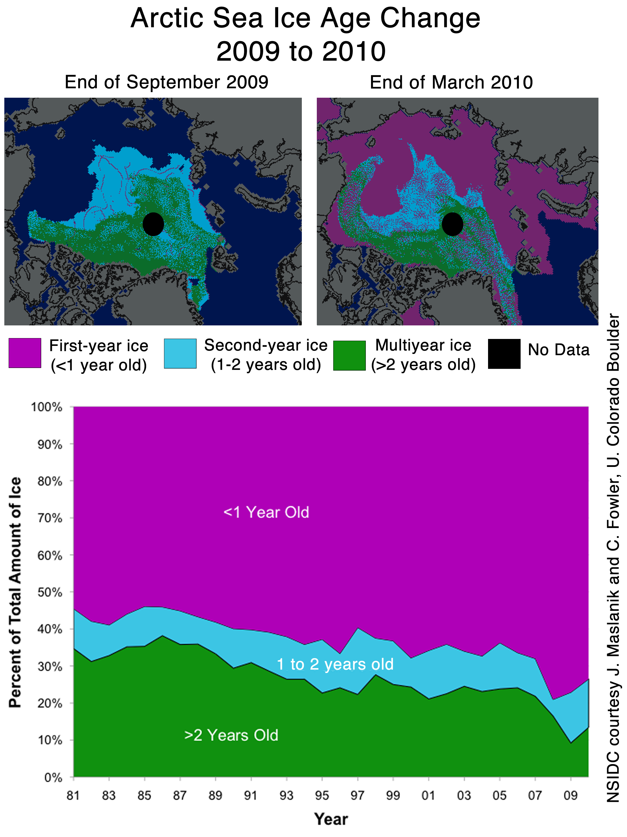
The areas that in recent years have been first-year ice that are now covered by 2nd and 3rd year ice will increase the volume – in those regions. However, compared to the last two years, there is even less of the oldest ice (see images below – I also included 1985 as an example of 1980s ice conditions for comparison). The loss of the oldest, thickest ice may more than offset the gain in volume from the 2nd and 3rd year ice. Also, it’s been a relatively warm winter in the Arctic, so first-year ice is likely a bit thinner than in recent years. Finally, the extent has been less than the last two years for the past couple of months. So the PIOMAS estimate that we are at record low volume anomaly is not implausible.

Early May ice age for: 1985 (top-left), 2008 (top-right), 2009 (bottom-left), and 2010 (bottom-right). OW = open water (no ice); 1 = ice that is 0-1 year old (first-year ice), 2 = ice that is 1-2 years old (2nd year ice), etc. Images courtesy of C. Fowler and J. Maslanik, University of Colorado, Boulder. Updated from Maslanik et al., 2007.
What does this all mean for this year’s minimum? Well, much will depend on the weather for the rest of the summer. As NSIDC states in its most recent post, we’ve expected we may see the rapid decline begin to slow because the melt will soon run into older, thicker ice, which will slow the loss of ice. Steve has said essentially the same thing and indeed we’ve the rate of loss slow over the past few days. Of course, there still a lot of time left in the melt season, and pace of melt continue to be relatively slow or it may speed up again, so we’ll see what happens. Regardless of what happens this summer though, the most important fact is that, despite some areas of the Arctic being a bit thicker this year, the long-term thinning and declining summer ice extent trend continues.
One final note about both PIPS and PIOMAS: Steve has claimed that “everyone agrees that PIPS 2.0 is the best data source of historical ice thickness”. Well, no scientist would even agree that what PIPS 2.0 produces are data! Being a data person myself, this is a bit of a pet peeve, but it’s important to make the distinction that model outputs are not data. Models are tremendously useful for obtaining information where data doesn’t exist (i.e., data sparse regions, historical periods without data), for projecting future changes, and for understanding how physical processes interact with each other (e.g., changes in climate due to changes in forcings).
However, model results are simulations, not observed data. And if there is good data available, I trust data over model estimates. And there is good historical data on ice thickness from submarine and satellite records (Kwok and Rothrock, 2009) and from proxy thickness estimates from ice age data (e.g., Maslanik et al., 2007). These data clearly show a long-term thinning trend. And while 2010 has relatively less of the thinner, first-year ice than the last couple of years, the ice cover is still much thinner than it was in earlier years. And it is clear that the models don’t entirely capture the spatial distribution of thickness correctly. As an example, compare the first-year ice in the ice age figure above with the PIPS 2.0 estimate from the same time period (below). In May, PIPS showed most of the central Arctic covered by ~3+ m ice, all the way to the Siberian coast. This is simply not realistic because the ice age data indicate first-year ice on much of the Siberian side of the Arctic (see images above), which would average at most 2 m. Thus Steve’s comparison of May 2010 and May 2008 with PIPS data is not valid because the model results are capturing observed spatial patterns of thickness.

References
Kwok , R. and D.A. Rothrock, 2009. Decline in Arctic sea ice thickness from submarine and ICESat records: 1958–2008, Geophys. Res. Lett., 36, L15501, doi:10.1029/2009GL039035.
Maslanik, J.A., C. Fowler, J. Stroeve, S. Drobot, J. Zwally, D. Yi, and W. Emery, 2007. A younger, thinner Arctic ice cover: Increased potential for extensive sea-ice loss, Geophys. Res. Lett., 34, L24501, doi:10.1029/2007GL032043.
Key PIPS 2.0 Model references:
Cox, M., 1984. A primitive equation, 3-dimensional model of the ocean, Geophysical Fluid Dynamics Laboratory Ocean Group Technical Report, Princeton, NJ, 1141 pp.
Hibler, W.D. III, 1979. A dynamic thermodynamic sea ice model, J. Phys. Oceanogr., 9(4), 815-846.
Hibler, W.D. III, 1980. Modeling a variable thickness sea ice cover, Mon. Weather Rev., 108(12), 1943-1973.
Thorndike, A.S., D.A. Rothrock, G.A. Maykut, and R. Colony, 1975. The thickness distribution of sea ice, J. Geophys. Res., 80(33), 4501-4513.
Key PIOMAS Model references:
Dukowicz, J.K., and R.D. Smith, 1994. Implicit free-surface method for the Bryan-Cox-Semtner ocean model, J. Geophys. Res., 99, 7791-8014.
Winton, M., 2000. A reformulated three-layer sea ice model, J. Atmos. Oceanic Technol., 17, 525-531.
Zhang J., and W.D. Hibler III, 1997. On an efficient numerical method for modeling sea ice dynamics, J. Geophys. Res., 102, 8691-8702.
Zhang, J., and D.A. Rothrock, 2001. A thickness and enthalpy distribution sea-ice model, J. Phys. Oceanogr., 31, 2986-3001.
Zhang, J., and D.A. Rothrock, 2003. Modeling global sea ice with a thickness and enthalpy distribution model in generalized curvilinear coordinates, Mon. Weather Rev., 131, 845-861.
PIPS versus PIOMAS: Deductive versus Inductive (a.k.a. Karl Popper)
The comparison of PIPS with PIOMAS is a good way to illustrate the deductive or inductive nature of scientific method as set out by Karl Popper in books such as “Conjectures and Refutations”. PIPS and PIOMAS are good examples of the deductive versus inductive scientific methods, respectively.
Of course it was one of Popper’s main conclusions that true scientific method could only be deductive and not inductive, and that in the end inductive inferences are an illusion. This was in parallel to an connected with Popper’s statement that for a theory or “conjecture” to be considered scientific, it must be falsifiable.
First, what do deductive and inductive mean? Approximately, deductive means disproving – believing a conjecture until it is disproved, then not believing it any more. Inductive means building a series of assumptions on each other in a complex structure without a clear possibility of falsification.
I looked at some dictionary definitions and other reference sources about these two words, inductive and deductive, since their meanings might be slipping and blurring. Inductive is linked to synthetic and synthesis while deductive was linked to analysis and analytic. I like to think of it in terms of the length of the paths that one draws between observation and conclusion. Short and economic (“parsimonious”) = deductive; long and convoluted involving multiple serial assumptions = inductive.
Finally “inductive” and “deductive” can be illustrated as follows. Two teams of scientists, team inductive and team deductive, were given a task: design a speedometer for a car – a device for measuring and displaying the speed that a car is travelling.
So team inductive got to work. This team included a fair number of physicists with computational and modelling skills. It became immediately clear to them that this was a task requiring the procesing of multiple factors all impacting on speed: what was the energy and force driving the car forward, what was the origin of this energy? Chemical and thermodynamic energy from the combustion of fuel needed to be carefully evaluated and modelled. What was the efficiency of this conversion from chemical to kinetic energy – how much was lost in the inefficiency of the motor?
Several team members were assigned to modelling these processes. How much energy was lost as friction and heat through the gas exhaust? Simulation of the turbulent fluid flow and associated heat fluxes along the exhaust pipe was clearly called for.
Then of course there were hours of immense fun to be had modelling and evaluating the fluid friction of the air passing over the car. This of course was modified by the dynamics of the air itself – what was the prevailing wind direction?
Then there was the question of how you define the spatial relationship between the car and the ground, whether to adopt a merely Cartesian or a Euclidian or relativistic or any other geometric frame of reference? Then of course there was the friction between the tyre and the road.
So it became clear to team inductive that to have any hope whatsoever of measuring speed in a credible way, to give an output that would be accepted by internationally recogonised car speed scientists associated with the high profile journals and societies, that a large number of data inputs were needed: chemical measurement probes in the fuel tank to asses the fuel chemical potential energy; probes within the ignition chamber to assess on a millisecond basis pressures and temperatures to illucidate combustion energy. Then multiple sensors were required in the exhaust pipe to
provide input for fluid flow modelling of the exhaust gasses. Sensors were also required at many locations on the car’s surface to assess airflow and boundary layer turbulence, as the exact location of the laminar-turbulent transition was a key factor in getting the drag models to work reliably. Sensors were needed within the tyres also. Other factors and associated sensor inputs were also identified and subject to in-depth research and computer simulation.
Thus at the end of the day it was deemed impossible to prove that the “speed” of the car that one measured was correct or not, or that the car was in fact moving at all, or whether it was even in contact with the road, and indeed what it was exactly that one meant by the concept of a “road”.
Then team deductive got to work. They measured the circumferance of the wheels. And set up a sensor to measure the rate of rotation of the wheels. From this they got a speedometer.
So PIPS fits the bill as a deductive method – simple, but it gives reliable results. As Walt Meier himself says, good for “operational” uses i.e. when the results actually matter, e.g. navigating on a ship. PIOMAS is by contrast inductive. That is why it does not work.
The inductive approach is not necessarily completely useless. The PIOMAS type model could be used to try to understand Arctic ice processes, just as “team inductive’s” model could be used for basic research into how a car behaves. But this is not the same thing as making robust and reliable measurements of a parameter. Confusion between research modelling and measurement of an environmental parameter is one of the weaknesses of the AGW approach to climate. Plus not having read and understood Popper.
From: EFS_Junior on July 14, 2010 at 2:21 pm
Nah, what one has is a big steaming pile.
If you have volume and area you can calculate average thickness. But does one have the area? According to IARC/JAXA:
You can’t use extent data as that uses ice concentration, so if a given measured area has 20% sea ice you would only use 20% of that area towards the sea ice total. IARC/JAXA has archived daily extent numbers and concentration maps, NSIDC has daily extent maps without a number and concentration maps which are not archived. Guess you could always count pixels off the concentration maps once you figure out how much area each pixel covers. The NSIDC archives do have monthly area figures, for whatever that’s worth.
Well, assuming you have usable area figures, then you need the volume data. Okay, where is it? From PIOMAS comes the terrifying Arctic Sea Ice Volume Anomaly chart, which has remained stuck at June 18 displaying the unprecedented long dead-straight drop. But that shows the anomaly, we need the actual numbers. On the PIOMAS main volume page we find… nothing daily, no archived volume figures, not even monthly. On Zhang’s site we find… no volume data, and some data files that are not current related to the “retrospection” of the Arctic sea ice. The volume numbers aren’t available.
So, where are we at? Can’t get the PIOMAS volume numbers anyway, and if there is daily area info available it won’t be coming from IARC/JAXA or NSIDC.
Then we get to how you’re mixing systems. Item one: Does the region that PIOMAS considers to have “Arctic sea ice” match up with the regions IARC/JAXA or NSIDC use?
Item two: Are you mixing algorithms? We often see how the same satellite data yields different extent figures due to the algorithms processing the data. Volume is not measured directly, PIOMAS calculates it, and somewhere along the way it has to be figuring out what the area is. Is there a mismatch? Well, the PIOMAS main page says they use the sea ice concentration data from the NSIDC near-real time product so the NSIDC daily area figures would be indicated. If such were available.
Note the “disclaimer” about the NSIDC near-real-time data:
What does that mean? According to the NSIDC, PIOMAS is using the wrong data.
Finally, why do you want to compound errors? While calculating volume, PIOMAS must have also calculated thickness. So why reverse-calculate from volume to get something used to calculate volume? Why not just use the PIOMAS thickness info which is available… Oh yeah, it isn’t available.
Well, as you said, if you had volume data and area data you could calculate thickness, albeit average thickness. So to do what PIPS already does and show you what the thickness is at a certain general area you would… need volume data for that certain general area. Got any?
Matthew L says: July 14, 2010 at 5:36 pm
Well I am glad you know how to find a web dictionary. Unfortunately you do not appear to have read it. One definition is:
“7. A state of extreme difficulty, pressure, or strain”.
There is no data that has significantly determined that an ice-free Arctic will endanger species. Because according to you, the Arctic has never been ice-free before. Or has it?
Mann, you’re stressing me out.
Have you looked at the posted source code? The PIOMAS code is not available, and offhand I do not see anything there that is indicated as actually used in PIOMAS. For example, the sole link to actual code says it’s for a Global sea Ice Model (GIM).
This must be indicative of that enormous chasm between scientists and engineers. I would have thought the distinction would be between model data and measured (or calculated from measured) data. Imagine how that would sound otherwise: “Here’s the wind tunnel data, and it matches pretty well with these numbers the model cranked out that aren’t data.” One needs to keep track of which is which and accept that model results are secondary to real-world measurements, but otherwise the use of that word to keep them distinct seems rather artificial.
And am I expected to believe no scientist at all ever talks about “the model data” when referring to the output?
Found at noaa.gov:
Hey look, links to Coupled Climate Model data are there.
The PIOMAS main page says:
At the NSIDC site it says:
You would so trust a product when the NSIDC itself is saying the product is using data unsuitable for the product’s results?
Tim Clark says:
July 15, 2010 at 8:20 am
Pardon? Me? I have not ventured an opinion here on whether the Arctic has been ice free in the past or not. You must be thinking of someone else.
Anyway it is a matter of fact that the Arctic has been ice free in the (distant) past. My problem is not that it will be ice free again, just that it is man’s selfish disregard for his environment that will make it so – and very quickly too. And it is this speed of change that will put most stress on animal populations, which generally need many hundreds of generations in order to adapt.