Some people cite scientists saying there is a “CO2 control knob” for Earth. No doubt there is, but due to the logarithmic effect of CO2, I think of it like a fine tuning knob, not the main station tuner. That said, a new data picture is emerging of an even bigger knob and lever; a nice bright yellow one.

A few months back, I found a website from NOAA that provides an algorithm and downloadable program for spotting regime shifts in time series data. It was designed by Sergei Rodionov of the NOAA Bering Climate and Ecosystem Center for the purpose of detecting shifts in the Pacific Decadal Oscillation.
Regime shifts are defined as rapid reorganizations of ecosystems from one relatively stable state to another. In the marine environment, regimes may last for several decades and shifts often appear to be associated with changes in the climate system. In the North Pacific, climate regimes are typically described using the concept of Pacific Decadal Oscillation. Regime shifts were also found in many other variables as demonstrated in the Data section of this website (select a variable and then click “Recent trends”).
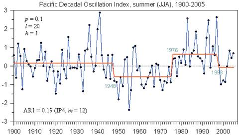
But data is data, and the program doesn’t care if it is ecosystem data, temperature data, population data, or solar data. It just looks for and identifies abrupt changes that stabilize at a new level. For example, a useful application of the program is to look for shifts in weather data, such as that caused by the PDO. Here we can clearly see the great Pacific Climate Shift of 1976/77:
Another useful application is to use it to identify station moves that result in a temperature shift. It might also be applied to proxy data, such as ice core Oxygen 18 isotope data.
But the program was developed around the PDO. What drives the PDO? Many say the sun, though there are other factors too. It follows to reason then the we might be able to look for solar regime shifts in PDO driven temperature data.
Alan of AppInSys found the same application and has done just that, and the results are quite interesting. The correlation is well aligned, and it demonstrates the solar to PDO connection quite well. I’ll let him tell his story of discovery below. – Anthony
=================================
Climate Regime Shifts
The notion that climate variations often occur in the form of ‘‘regimes’’ began to become appreciated in the 1990s. This paradigm was inspired in large part by the rapid change of the North Pacific climate around 1977 [e.g., Kerr, 1992] and the identification of other abrupt shifts in association with the Pacific Decadal Oscillation (PDO) [Mantua et al., 1997].” [http://www.beringclimate.noaa.gov/regimes/Regime_shift_algorithm.pdf]
Pacific Regime Shifts
Hare and Mantua, 2000 (“Empirical evidence for North Pacific regime shifts in 1977 and 1989”): “It is now widely accepted that a climatic regime shift transpired in the North Pacific Ocean in the winter of 1976–77. This regime shift has had far reaching consequences for the large marine ecosystems of the North Pacific. Despite the strength and scope of the changes initiated by the shift, it was 10–15 years before it was fully recognized. Subsequent research has suggested that this event was not unique in the historical record but merely the latest in a succession of climatic regime shifts. In this study, we assembled 100 environmental time series, 31 climatic and 69 biological, to determine if there is evidence for common regime signals in the 1965–1997 period of record. Our analysis reproduces previously documented features of the 1977 regime shift, and identifies a further shift in 1989 in some components of the North Pacific ecosystem. The 1989 changes were neither as pervasive as the 1977 changes nor did they signal a simple return to pre-1977 conditions.”
[http://www.sciencedirect.com/science?_ob=ArticleURL&_udi=B6V7B-41FTS3S-2…]
Overland et al “North Pacific regime shifts: Definitions, issues and recent transitions”
[http://www.pmel.noaa.gov/foci/publications/2008/overN667.pdf]: “climate variables for the North Pacific display shifts near 1977, 1989 and 1998.”
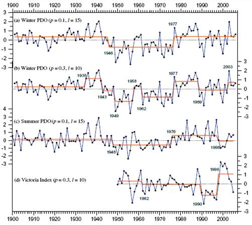
The following figure from the above paper show analysis of PDO and Victoria Index using the Rodionov regime detection algorithm. A regime shift is also detected around 1947-48.
The following figure shows regime shift detection for the summer PDO, showing shifts at 1948, 1976 and 1998.
[http://www.beringclimate.noaa.gov/data/Images/PDOs_FigRegime.html]
(For detailed information on the 1976/77 climate shift,
see: http://www.appinsys.com/GlobalWarming/The1976-78ClimateShift.htm)
Regime Shift Detection in Annual Temperature Anomaly Data
The NOAA Bering Climate web site provides the algorithm for regime shift detection developed by Sergei Rodionov [http://www.beringclimate.noaa.gov/regimes/index.html]. The following analyses use the Excel VBA regime change algorithm version 3.2 from this web site.
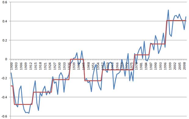
The following figure shows the regime analysis of the HadCRUT3 annual global annual average temperature anomaly data from the Met Office Hadley Centre for 1895 to 2009 [http://hadobs.metoffice.com/hadcrut3/diagnostics/global/nh+sh/annual].
The analysis was run based on the mean using a significance level of 0.1, cut-off length of 10 and Huber weight parameter of 2 using red noise IP4 subsample size 6. Regime changes are identified in 1902, 1914, 1926, 1937, 1946, 1957, 1977, 1987, and 1997. Running the analysis based on the variance rather than the mean results in regime changes in the bold years listed above.
Regime Shift Relationship to Solar Cycle
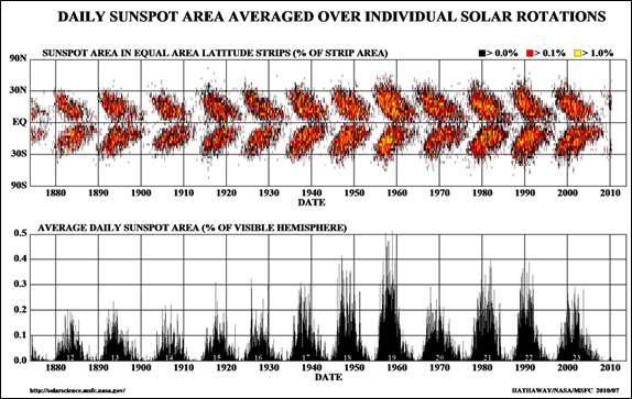
The NASA Solar Physics web site provides the following figure showing sunspot area.
[http://solarscience.msfc.nasa.gov/SunspotCycle.shtml]
The following figure compares the Hadley (HadCrut3) monthly global average temperature (from [http://hadobs.metoffice.com/hadcrut3/diagnostics/global/nh+sh/]) overlaid with the regime change line (red line) shown previously, along with the sunspot area since 1900. The sunspot cycle is approximately 11 years. The sun’s magnetic field reverses with each sunspot cycle and thus after two sunspot cycles the magnetic field has completed a cycle – a Hale Cycle – and is back to where it started. Thus a complete magnetic sunspot cycle is approximately 22 years. The figure marks the onset of odd-numbered cycles with a vertical red line, even-numbered cycles with a green line.
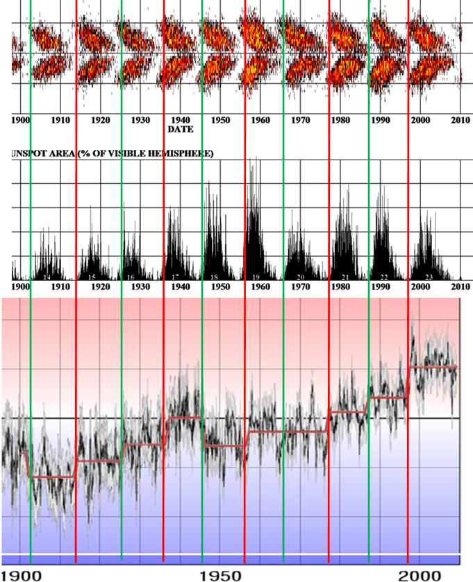
From the figure above it can be seen that the regime changes correspond to the onset of solar cycles and occur when the “butterfly” is at its widest. The most significant warming regime shifts occur at the start of odd-numbered cycles (1937, 1957, 1977, 1997). Each odd-numbered cycle (red lines above) has resulted in a temperature-increase regime shift. Even-numbered cycles (green lines above) have been inconsistent, with some resulting in temperature-decrease regime shifts (1902, 1946) or minor temperature-increase shifts (1926, 1987).
An unusual one is the 1957 – 1966 cycle, which in the monthly data shown above visually looks like a temperature-increase shift in 1957 followed by a temperature-decrease shift in 1964 but the regime detection algorithm did not identify it. This is likely due to the use of annually averaged data in the regime detection algorithm.
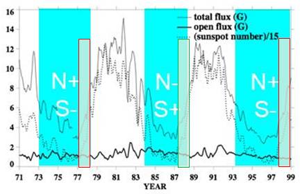
The following figure shows the relative polarity of the Sun’s magnetic poles for recent sunspot cycles along with the solar magnetic flux [www.bu.edu/csp/nas/IHY_MagField.ppt]. The regime change periods are highlighted by the red and green boxes. Each one occurs on as the solar cycle is accelerating. The onset of an odd-numbered sunspot cycle (1977-78, 1997-98) results in the relative alignment of the Earth’s and the Sun’s magnetic fields (positive North pole on the Sun) allowing greater penetration of the geomagnetic storms into the Earth’s atmosphere. “Twenty times more solar particles cross the Earth’s leaky magnetic shield when the sun’s magnetic field is aligned with that of the Earth compared to when the two magnetic fields are oppositely directed” [http://www.nasa.gov/mission_pages/themis/news/themis_leaky_shield.html]
The following figure shows the longitudinally averaged solar magnetic field. This “magnetic butterfly diagram” shows that the sunspots are involved with transporting the field in its reversal. The Earth’s temperature regime shifts are indicated with the superimposed boxes – red on odd numbered solar cycles, green on even.
[http://solarphysics.livingreviews.org/open?pubNo=lrsp-2010-1&page=articlesu8.html]
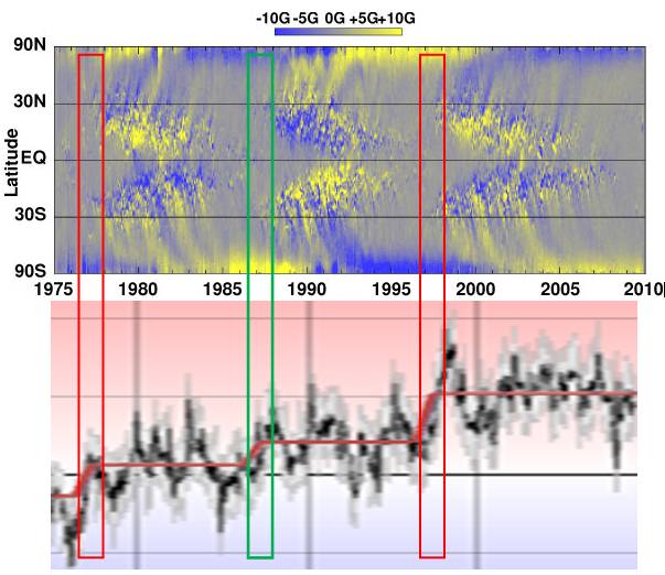
The Earth’s temperature regime shift occurs as the solar magnetic field begins its reversal.
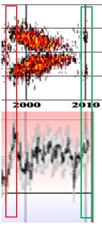
Solar Cycle 24
Solar cycle 24 is in its initial stage after getting off to a late start. An El Nino occurred in the first part of 2010. This may be the start of the next regime shift.
Climate Regime Shifts
[last update: 2010/07/04]
|
“The notion that climate variations often occur in the form of ‘‘regimes’’ began to become appreciated in the 1990s. This paradigm was inspired in large part by the rapid change of the North Pacific climate around 1977 [e.g., Kerr, 1992] and the identification of other abrupt shifts in association with the Pacific Decadal Oscillation (PDO) [Mantua et al., 1997].” [http://www.beringclimate.noaa.gov/regimes/Regime_shift_algorithm.pdf]
|
|
Pacific Regime Shifts
Hare and Mantua, 2000 (“Empirical evidence for North Pacific regime shifts in 1977 and 1989”): “It is now widely accepted that a climatic regime shift transpired in the North Pacific Ocean in the winter of 1976–77. This regime shift has had far reaching consequences for the large marine ecosystems of the North Pacific. Despite the strength and scope of the changes initiated by the shift, it was 10–15 years before it was fully recognized. Subsequent research has suggested that this event was not unique in the historical record but merely the latest in a succession of climatic regime shifts. In this study, we assembled 100 environmental time series, 31 climatic and 69 biological, to determine if there is evidence for common regime signals in the 1965–1997 period of record. Our analysis reproduces previously documented features of the 1977 regime shift, and identifies a further shift in 1989 in some components of the North Pacific ecosystem. The 1989 changes were neither as pervasive as the 1977 changes nor did they signal a simple return to pre-1977 conditions.” [http://www.sciencedirect.com/science?_ob=ArticleURL&_udi=B6V7B-41FTS3S-2…]
Overland et al “North Pacific regime shifts: Definitions, issues and recent transitions” [http://www.pmel.noaa.gov/foci/publications/2008/overN667.pdf]: “climate variables for the North Pacific display shifts near 1977, 1989 and 1998.”
The following figure from the above paper show analysis of PDO and Victoria Index using the Rodionov regime detection algorithm. A regime shift is also detected around 1947-48.
The following figure shows regime shift detection for the summer PDO, showing shifts at 1948, 1976 and 1998. [http://www.beringclimate.noaa.gov/data/Images/PDOs_FigRegime.html]
(For detailed information on the 1976/77 climate shift, see: http://www.appinsys.com/GlobalWarming/The1976-78ClimateShift.htm)
|
|
Regime Shift Detection in Annual Temperature Anomaly Data
The NOAA Bering Climate web site provides the algorithm for regime shift detection developed by Sergei Rodionov [http://www.beringclimate.noaa.gov/regimes/index.html]. The following analyses use the Excel VBA regime change algorithm version 3.2 from this web site.
The following figure shows the regime analysis of the HadCRUT3 annual global annual average temperature anomaly data from the Met Office Hadley Centre for 1895 to 2009 [http://hadobs.metoffice.com/hadcrut3/diagnostics/global/nh+sh/annual].
The analysis was run based on the mean using a significance level of 0.1, cut-off length of 10 and Huber weight parameter of 2 using red noise IP4 subsample size 6. Regime changes are identified in 1902, 1914, 1926, 1937, 1946, 1957, 1977, 1987, and 1997. Running the analysis based on the variance rather than the mean results in regime changes in the bold years listed above.
|
|
Regime Shift Relationship to Solar Cycle
The NASA Solar Physics web site provides the following figure showing sunspot area. [http://solarscience.msfc.nasa.gov/SunspotCycle.shtml]
The following figure compares the Hadley (HadCrut3) monthly global average temperature (from [http://hadobs.metoffice.com/hadcrut3/diagnostics/global/nh+sh/]) overlaid with the regime change line (red line) shown previously, along with the sunspot area since 1900. The sunspot cycle is approximately 11 years. The sun’s magnetic field reverses with each sunspot cycle and thus after two sunspot cycles the magnetic field has completed a cycle – a Hale Cycle – and is back to where it started. Thus a complete magnetic sunspot cycle is approximately 22 years. The figure marks the onset of odd-numbered cycles with a vertical red line, even-numbered cycles with a green line.
From the figure above it can be seen that the regime changes correspond to the onset of solar cycles and occur when the “butterfly” is at its widest. The most significant warming regime shifts occur at the start of odd-numbered cycles (1937, 1957, 1977, 1997). Each odd-numbered cycle (red lines above) has resulted in a temperature-increase regime shift. Even-numbered cycles (green lines above) have been inconsistent, with some resulting in temperature-decrease regime shifts (1902, 1946) or minor temperature-increase shifts (1926, 1987).
An unusual one is the 1957 – 1966 cycle, which in the monthly data shown above visually looks like a temperature-increase shift in 1957 followed by a temperature-decrease shift in 1964 but the regime detection algorithm did not identify it. This is likely due to the use of annually averaged data in the regime detection algorithm.
The following figure shows the relative polarity of the Sun’s magnetic poles for recent sunspot cycles along with the solar magnetic flux [www.bu.edu/csp/nas/IHY_MagField.ppt]. The regime change periods are highlighted by the red and green boxes. Each one occurs on as the solar cycle is accelerating. The onset of an odd-numbered sunspot cycle (1977-78, 1997-98) results in the relative alignment of the Earth’s and the Sun’s magnetic fields (positive North pole on the Sun) allowing greater penetration of the geomagnetic storms into the Earth’s atmosphere. “Twenty times more solar particles cross the Earth’s leaky magnetic shield when the sun’s magnetic field is aligned with that of the Earth compared to when the two magnetic fields are oppositely directed” [http://www.nasa.gov/mission_pages/themis/news/themis_leaky_shield.html]
The following figure shows the longitudinally averaged solar magnetic field. This “magnetic butterfly diagram” shows that the sunspots are involved with transporting the field in its reversal. The Earth’s temperature regime shifts are indicated with the superimposed boxes – red on odd numbered solar cycles, green on even. [http://solarphysics.livingreviews.org/open?pubNo=lrsp-2010-1&page=articlesu8.html]
The Earth’s temperature regime shift occurs as the solar magnetic field begins its reversal.
|
|
Solar Cycle 24
Solar cycle 24 is in its initial stage after getting off to a late start. An El Nino occurred in the first part of 2010. This may be the start of the next regime shift.
|
Vuk etc. says:
July 10, 2010 at 10:39 am
At lower V (as far as I remember) electron is still attached to nucleus and will radiate IR, as V increases electron moves up the range of levels, radiation moves from IR towards UV, eventually electron is removed from nucleus.
If the sun has not V available it has other sources of energy.
There is no voltage V doing anything. The process is completely different from a discharge tube. The radiation from the photosphere is controlled by the negative Hydrogen ion [H-], which varies with wave length. The process in involved and a full explanation cannot easily be given here, but can be found in any good textbook about the Sun. I recommend ISBN 978-1-4200-8307-1 by Dermott J. Mullan.
Hydride (H anion, H-) was all the rage with water purifying people. There are two ways H- can be produced; 2H splits into H+ and H- when electron escapes from the first one to the second, or H acquires a free floating electron to become H-.
What you plasma people do with all those Hs I have no idea, but laws of physics must be obeyed.
Vuk etc. says:
July 10, 2010 at 12:22 pm
What you plasma people do with all those Hs I have no idea, but laws of physics must be obeyed.
And they are in this particular case.
Stephen Wilde: My question, “Based on your observations, how many degrees latitude are the variations in polar cycles (AO & SAM) pushing the clouds equatorward in response to decreasing solar activity?”
Your reply, “Exactly what I would like to know. Where can I find the data ?”
I find your question rather remarkable since a major part of your hypothesis is based on the non-seasonal latitudinal variation in the ITCZ. You could use CAMSOPI precipitation data or ISCCP cloud amount data. The CAMSOPI precipitation data does a much better job if representing the latitude of the ITCZ. Both are available through the KNMI Climate Explorer. For months, I have repeatedly suggested to you that you verify your claims with data. We know that the AO is not correlated with the solar cycle over any time period when data is available. Refer to AO and Sunspot Number data starting in 1950:
http://i40.tinypic.com/fkr5n6.png
And refer to data starting in 1900:
http://i40.tinypic.com/2mc7eki.png
Would you be concerned if you were to discover that there is no correlation between the latitude of the ITCZ and Sunspot Number or the latitude of the ITCZ and the AO? You need to verify your claims with data, Stephen.
You replied, “By the way, have you noticed that Roy Spencer on his website seems to be using the term PDO in the way that you so objected to when I did it ?”
That’s an assumption on your part. His use of the PDO also reflects the proper definition of it, which is why I always question his use of it.
@Leif Svalgaard says:
July 10, 2010 at 8:02 am
“No, not likely as the IR level changes are progressing steadily while solar wind speed varies intermittently [in bursts], but we don’t know yet. This data is very new, not even covering a full cycle yet.”
Who has this data, and is it available?
Ulric Lyons says:
July 10, 2010 at 3:08 pm
Who has this data, and is it available?
http://lasp.colorado.edu/sorce/data/ssi_data.htm
“Would you be concerned if you were to discover that there is no correlation between the latitude of the ITCZ and Sunspot Number or the latitude of the ITCZ and the AO? ”
Not concerned but my hypothesis would be rather shaky.
However we do know that the ITCZ was nearer the equator in the depths of the LIA and that it has a moved poleward since. Likewise the mid latitude jets.
Also that in the MWP the jets must have been more poleward than now to allow Viking agriculture in Greenland.
We also know that when the AO is positive the jets drift poleward and vice versa.
The trouble is that we don’t have enough data on all three components until far too recently for the situation to be clear. After all we are considering a 500 to 1000 year cycle which is pretty much drowned out for periods less than 30 years.
The information we do have fits my hypothesis and all we need to prove or refute it is some continuing observation with our modern methods. For the past 10 years the fit has held good. As the sun has become quieter so has the AO in general become more negative and the jets have sunk equatorward.
Bob Tisdale said:
“We know that the AO is not correlated with the solar cycle over any time period when data is available. Refer to AO and Sunspot Number data starting in 1950:
http://i40.tinypic.com/fkr5n6.png
And refer to data starting in 1900:
http://i40.tinypic.com/2mc7eki.png”
Quite so. ‘When data is available’ is the key point.
And I have said we also need to key in the ocean cycles i.e. the net state of all the global oceans combined at any given time. Not just ENSO. All will have an effect on the jet stream positioning. No one knows the net global situation at any given time.
And I told you the oceanic effect is greater than the solar effect. We do not know by how much.
The data we have is not helpful. We need to watch and learn instead of extrapolating from inadequate data. Hopefully someone will note what I say and start recording something useful but as I said I’ve made the position very clear. Anyone will be able to see as we go along whether events broadly support me or definitively falsify what I say.
Patience.
Stephen Wilde says:
July 10, 2010 at 4:20 pm
And I told you the oceanic effect is greater than the solar effect. We do not know by how much.
If you do not know by how much, how can you say it is ‘greater’?
Bob Tisdale says:
July 10, 2010 at 1:07 pm
Stephen Wilde: My question, “Based on your observations, how many degrees latitude are the variations in polar cycles (AO & SAM) pushing the clouds equatorward in response to decreasing solar activity?”
Ill posed problems,ie multiple time series.
Firstly would it not be more correct to examine when say radiative forcing ( insolation ) is greatest, which would be the inter annual solar cycle.Here the annual excursions of the extratropical storm tracks with their latitudinal effects are well described in the literature eg Ramanathan
The enormous cooling effect of extratropical storm track cloud systems
Extra-tropical storm track cloud systems provide about 60% of the total cooling effect of clouds [2]. The annual mean forcing from these cloud systems is in the range of –45 to –55 W m–2 and effectively these cloud systems are shielding both the northern and
the southern polar regions from intense radiative heating. Their spatial extent towards the tropics moves with the jet stream, extending farthest towards the tropics
(about 35 deg latitude) during winter and retreating polewards (polewards of 50 deg
latitude) during summer. This phenomenon raises an important question related to past climate dynamics. During the ice age, due to the large polar cooling, the northern hemisphere jet stream extended more southwards. But have the extra tropical cloud systems also moved southward? The increase in the negative forcing would have exerted a major positive feedback on the ice age cooling. There is a curious puzzle about the existence of these cooling clouds. The basic function of the extra tropical dynamics is to export heat polewards.
While the baroclinic systems are efficient in transporting heat, the enormous negative
radiative forcing (Fig. 2) associated with these cloud systems seems to undo the
poleward transport of heat by the dynamics. The radiative effect of these systems is working against the dynamical effect. Evidently,we need better understanding of the dynamic-thermodynamic coupling between these enormous cooling clouds and the
equator-pole temperature gradient, and greenhouse forcing.
This now introduces a number of binary problems (yes/no), in the 11 yr solar cycle (where we are told that an arbitary temperature signal occurs ) is this an increase in forcing or a decrease in dissipation ? ( atmospheric polar heat transport) . Why do significant temperature excursions occur around minima eg 1997 , and now?
The next step is to examine the stream function (jets) and what occurs say in a meteorological series . This is also well described in the literature eg Bals-Elsholz et al.
A distinct characteristic of the climatological time mean flow during winter in the Southern Hemisphere (SH) is the presence of a split jet at the longitudes of
Australia and New Zealand. The equatorward branch of the time-mean split jet is anchored by a strong subtropical jet (STJ) that extends eastward between 25s and
30S from the central South Indian Ocean across Australia to the east-central South Pacific Ocean near 130W. A zone of weak westerlies lies poleward of theSTJ from southeastern Australia eastward across the South Island of New Zealand to east of the date line.
As the STJ moves northward in perturbed SH spring a regime of blocking highs appear above the South Pacific convergence zone (35s) and blocking mid southern latitudes from transport, this is evident in Chatham Islands station in 2009 (44s)
http://i255.photobucket.com/albums/hh133/mataraka/chathamhadcrugiss2009.png
Hence interesting questions arise.
Stephen Wilde replied, “The data we have is not helpful. ”
The only reason data is not helpful to you is because it contradicts and disproves your ramblings. It is helpful to anyone who is interested in actually determining how climate might work.
maksimovich: Thanks for the write-up. But Stephen Wilde’s conjectures are based on non-seasonal variability. Do you have a link to that full paper or is it part of a book? I’d like to see how the author accounts for the impacts of ENSO on seasonal variability.
Stephen Wilde: You replied, “Quite so. ‘When data is available’ is the key point.”
If the data doesn’t agree with your NCM over three solar cycles and it doesn’t agree with your NCM over 9 solar cycles, extending the data back in time won’t help because you’ve still got those two periods when the data disagrees with your NCM.
You wrote, “Hopefully someone will note what I say and start recording something useful but as I said I’ve made the position very clear. Anyone will be able to see as we go along whether events broadly support me or definitively falsify what I say.”
The data is there, Stephen. I’ve pointed you to it a number of times. It is very useful to those who take the time to download it, interpret it and understand it. You don’t bother, and that is telling, especially in an area of science that is data dependent. As I’ve writen before, since you fail to present data, your conjectures cannot be verified or disproved, and your hypotheses are, therefore, meaningless.
Leif Svalgaard says:
July 10, 2010 at 10:57 am (Edit)
I recommend ISBN 978-1-4200-8307-1 by Dermott J. Mullan.
You solar physicists come up with catchy titles for books don’t you?
“Physics of the Sun: A First Course”
tallbloke says:
July 10, 2010 at 9:48 pm
“Physics of the Sun: A First Course”
But it is good.
@Stephen Fisher Wilde says:
July 10, 2010 at 4:20 pm
Bob Tisdale said:
“We know that the AO is not correlated with the solar cycle over any time period when data is available. Refer to AO and Sunspot Number data starting in 1950:
http://i40.tinypic.com/fkr5n6.”
The 17yr coronal hole cycle (and half cycle) in the AO data in the above graph link?
“And I have said we also need to key in the ocean cycles i.e. the net state of all the global oceans combined at any given time. Not just ENSO. All will have an effect on the jet stream positioning. No one knows the net global situation at any given time.
And I told you the oceanic effect is greater than the solar effect. We do not know by how much.”
Year to year, or season by season, definitely not, at this scale the Sun dominates jet steam position, and weather effects.
“Leif Svalgaard says:
July 10, 2010 at 4:25 pm
Stephen Wilde says:
July 10, 2010 at 4:20 pm
And I told you the oceanic effect is greater than the solar effect. We do not know by how much.
If you do not know by how much, how can you say it is ‘greater’?”
Well that’s easy. The oceanic effect appears to be clear on much shorter timescales. The jets are currently a bit more poleward from the recent El Nino than they were from the previous La Nina despite the quiet sun. I don’t agree with Ulric on that point.
Against that the jets didn’t go so far poleward as they did in the late 20th century from similar El Nino events.
So the oceanic effect is the primary one in the short term but the solar effect plays a role in modulating it especially over longer time periods
When one gets to a 500 year time scale then the solar effect dominates hence the cycle MWP to LIA to recent warming spell.
“Bob Tisdale says:
July 10, 2010 at 6:59 pm
Stephen Wilde: You replied, “Quite so. ‘When data is available’ is the key point.”
If the data doesn’t agree with your NCM over three solar cycles and it doesn’t agree with your NCM over 9 solar cycles, extending the data back in time won’t help because you’ve still got those two periods when the data disagrees with your NCM.”
That data does not deal with all the variables namely the level of solar activity, the stato of the AO, the net global contribution of ALL the oceans combined and an accurate assessment of the jet stream response. The data is inadequate.
Ulric Lyons:
I can’t agree with you that the sun has the dominant effect on any time scale because the oceans are so much more powerful in moving the jets latitudinally. However it may be that individual solar surface events could affect weather by affecting the wiggling of the jets once the current latitudinal position has been set by the combined solar and oceanic balance.
Even so I don’t see how one could distinguish any such solar effects (if they do occur) from weather events arising from normal chaotic variability.
Still, I support your right to try.
Ulric Lyons: You wrote in reply to Stephen Wilde, “The 17yr coronal hole cycle (and half cycle) in the AO data in the above graph link?”
You’d have to supply the coronal hole cycle data and compare it to the AO data since I’ve never heard of the “17yr coronal hole cycle (and half cycle)”. I don’t believe I’ve ever heard Leif discuss it or seen it discussed on a thread in which he is commenting.
You wrote, “Year to year, or season by season, definitely not, at this scale the Sun dominates jet steam position, and weather effects.”
How do you account for the impacts of ENSO on jet stream position, since ENSO does not correlate with solar cycles and since ENSO is a major factor in year-to-year jet stream postition? Or are you discussing the seasonal positions of the jet streams? Stephen’s discussions of climate generally do not include seasonal variability.
Stephen Wilde says:
July 11, 2010 at 5:23 am
Well that’s easy. The oceanic effect appears to be clear on much shorter timescales.
Still no numbers, so how can you tell?
When one gets to a 500 year time scale then the solar effect dominates hence the cycle MWP to LIA to recent warming spell.
Except that the sun didn’t vary in concert with the temperature the past couple thousand years. See Figure 20 of http://www.leif.org/research/Does%20The%20Sun%20Vary%20Enough.pdf
Stephen Wilde wrote, “Against that the jets didn’t go so far poleward as they did in the late 20th century from similar El Nino events.” And you wrote, “When one gets to a 500 year time scale then the solar effect dominates hence the cycle MWP to LIA to recent warming spell.”
And on what reconstruction data of the jet stream location are you basing this?
And you wrote, “That data does not deal with all the variables namely the level of solar activity, the stato [sic] of the AO, the net global contribution of ALL the oceans combined and an accurate assessment of the jet stream response. The data is inadequate.”
That paragraph is remarkable, Stephen. If there is no “accurate assessment of the jet stream response”, on what are you basing your assumptions? Guesswork on your part? And that paragraph included in effect your opinions that sunspot numbers don’t reflect the level of solar activity and that the AO data does not represent the AO. Last, “the net global contribution of ALL the oceans combined” to what?
Stephen Wilde wrote, “That data does not deal with all the variables namely the level of solar activity, the stato of the AO, the net global contribution of ALL the oceans combined and an accurate assessment of the jet stream response. The data is inadequate.”
Your NCM states:
“Solar surface turbulence increases causing an expansion of the Earth’s atmosphere,” which through a few other processes (that Leif disputed) results in “…less resistance to energy flowing up from the troposphere so the polar high pressure systems shrink and weaken accompanied by increasingly positive Arctic and Antarctic Oscillations.”
And your NCM states, “Solar surface turbulence passes its peak and the Earth’s atmosphere starts to contract, ” and again through the disputed processes causes an “…increased resistance to energy flowing up from the troposphere so the polar high pressure systems expand and intensify producing increasingly negative Arctic and Antarctic Oscillations.”
Based on that description of your NCM, sunspot numbers (or TSI) should correlate with the Arctic Oscillation, and the two are not correlated.
And as I asked before, would it concern you to discover that the non-seasonal latitudinal position of the ITCZ is not correlated with the solar cycle?
Well gentlemen, this might help. I made month by month analysis of the CETs.
In UK in summer and autumn temperatures mainly respond to the sun, while in the winter and spring to the Gulf Stream. But it does not appear to be so clear cut. I have taken 300 year rising trend (mainly out of the winters, since there was very little or none in the summers), for easier comparison.
Here is the result
http://www.vukcevic.talktalk.net/CETm.htm
I hope you can see something in it since to me it appears that the summer months are slightly more in tune with the solar cycle.
@Stephen Fisher Wilde says:
July 11, 2010 at 5:29 am
Ulric Lyons:
“I can’t agree with you that the sun has the dominant effect on any time scale because the oceans are so much more powerful in moving the jets latitudinally. However it may be that individual solar surface events could affect weather by affecting the wiggling of the jets once the current latitudinal position has been set by the combined solar and oceanic balance.”
I get the feeling you are postulating this rather than basing it on observations, and anyway, your `oceanic balance` is driven by the solar changes, but if you are not concentrating on the relevent solar output, you would not notice this in the first place.
“Even so I don’t see how one could distinguish any such solar effects (if they do occur) from weather events arising from normal chaotic variability.”
There is no `normal chaotic variability` in weather events, they are all predictable and driven by the Sun.
@Bob Tisdale says:
July 11, 2010 at 6:17 am
Ulric Lyons: You wrote in reply to Stephen Wilde, “The 17yr coronal hole cycle (and half cycle) in the AO data in the above graph link?”
You’d have to supply the coronal hole cycle data and compare it to the AO data since I’ve never heard of the “17yr coronal hole cycle (and half cycle)”. I don’t believe I’ve ever heard Leif discuss it or seen it discussed on a thread in which he is commenting.
You wrote, “Year to year, or season by season, definitely not, at this scale the Sun dominates jet steam position, and weather effects.”
How do you account for the impacts of ENSO on jet stream position, since ENSO does not correlate with solar cycles and since ENSO is a major factor in year-to-year jet stream postition? Or are you discussing the seasonal positions of the jet streams? Stephen’s discussions of climate generally do not include seasonal variability.
___________________________________________________________
Yes it is very curious that so many learned folk presume the wrong things about the solar cycle and SSN, and overlook the dominant forcing factor, the solar wind and coronal holes.
I used a solar based forecast for the last El Nino and got it bang on, I did not refer to the solar cycle though.
If Stephens model does not include `seasonal variability` then it cannot be a climate model by definition, and would be useless for temperatures and jet stream position, and hydrology outlooks would be impossible.