Some people cite scientists saying there is a “CO2 control knob” for Earth. No doubt there is, but due to the logarithmic effect of CO2, I think of it like a fine tuning knob, not the main station tuner. That said, a new data picture is emerging of an even bigger knob and lever; a nice bright yellow one.

A few months back, I found a website from NOAA that provides an algorithm and downloadable program for spotting regime shifts in time series data. It was designed by Sergei Rodionov of the NOAA Bering Climate and Ecosystem Center for the purpose of detecting shifts in the Pacific Decadal Oscillation.
Regime shifts are defined as rapid reorganizations of ecosystems from one relatively stable state to another. In the marine environment, regimes may last for several decades and shifts often appear to be associated with changes in the climate system. In the North Pacific, climate regimes are typically described using the concept of Pacific Decadal Oscillation. Regime shifts were also found in many other variables as demonstrated in the Data section of this website (select a variable and then click “Recent trends”).
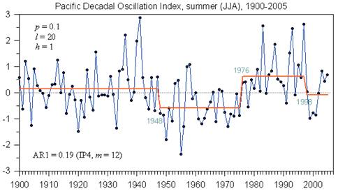
But data is data, and the program doesn’t care if it is ecosystem data, temperature data, population data, or solar data. It just looks for and identifies abrupt changes that stabilize at a new level. For example, a useful application of the program is to look for shifts in weather data, such as that caused by the PDO. Here we can clearly see the great Pacific Climate Shift of 1976/77:
Another useful application is to use it to identify station moves that result in a temperature shift. It might also be applied to proxy data, such as ice core Oxygen 18 isotope data.
But the program was developed around the PDO. What drives the PDO? Many say the sun, though there are other factors too. It follows to reason then the we might be able to look for solar regime shifts in PDO driven temperature data.
Alan of AppInSys found the same application and has done just that, and the results are quite interesting. The correlation is well aligned, and it demonstrates the solar to PDO connection quite well. I’ll let him tell his story of discovery below. – Anthony
=================================
Climate Regime Shifts
The notion that climate variations often occur in the form of ‘‘regimes’’ began to become appreciated in the 1990s. This paradigm was inspired in large part by the rapid change of the North Pacific climate around 1977 [e.g., Kerr, 1992] and the identification of other abrupt shifts in association with the Pacific Decadal Oscillation (PDO) [Mantua et al., 1997].” [http://www.beringclimate.noaa.gov/regimes/Regime_shift_algorithm.pdf]
Pacific Regime Shifts
Hare and Mantua, 2000 (“Empirical evidence for North Pacific regime shifts in 1977 and 1989”): “It is now widely accepted that a climatic regime shift transpired in the North Pacific Ocean in the winter of 1976–77. This regime shift has had far reaching consequences for the large marine ecosystems of the North Pacific. Despite the strength and scope of the changes initiated by the shift, it was 10–15 years before it was fully recognized. Subsequent research has suggested that this event was not unique in the historical record but merely the latest in a succession of climatic regime shifts. In this study, we assembled 100 environmental time series, 31 climatic and 69 biological, to determine if there is evidence for common regime signals in the 1965–1997 period of record. Our analysis reproduces previously documented features of the 1977 regime shift, and identifies a further shift in 1989 in some components of the North Pacific ecosystem. The 1989 changes were neither as pervasive as the 1977 changes nor did they signal a simple return to pre-1977 conditions.”
[http://www.sciencedirect.com/science?_ob=ArticleURL&_udi=B6V7B-41FTS3S-2…]
Overland et al “North Pacific regime shifts: Definitions, issues and recent transitions”
[http://www.pmel.noaa.gov/foci/publications/2008/overN667.pdf]: “climate variables for the North Pacific display shifts near 1977, 1989 and 1998.”
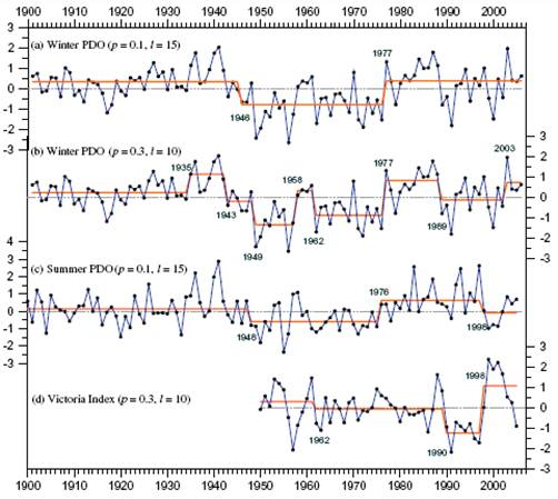
The following figure from the above paper show analysis of PDO and Victoria Index using the Rodionov regime detection algorithm. A regime shift is also detected around 1947-48.
The following figure shows regime shift detection for the summer PDO, showing shifts at 1948, 1976 and 1998.
[http://www.beringclimate.noaa.gov/data/Images/PDOs_FigRegime.html]
(For detailed information on the 1976/77 climate shift,
see: http://www.appinsys.com/GlobalWarming/The1976-78ClimateShift.htm)
Regime Shift Detection in Annual Temperature Anomaly Data
The NOAA Bering Climate web site provides the algorithm for regime shift detection developed by Sergei Rodionov [http://www.beringclimate.noaa.gov/regimes/index.html]. The following analyses use the Excel VBA regime change algorithm version 3.2 from this web site.
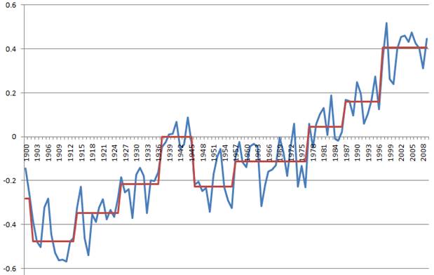
The following figure shows the regime analysis of the HadCRUT3 annual global annual average temperature anomaly data from the Met Office Hadley Centre for 1895 to 2009 [http://hadobs.metoffice.com/hadcrut3/diagnostics/global/nh+sh/annual].
The analysis was run based on the mean using a significance level of 0.1, cut-off length of 10 and Huber weight parameter of 2 using red noise IP4 subsample size 6. Regime changes are identified in 1902, 1914, 1926, 1937, 1946, 1957, 1977, 1987, and 1997. Running the analysis based on the variance rather than the mean results in regime changes in the bold years listed above.
Regime Shift Relationship to Solar Cycle
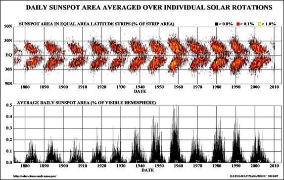
The NASA Solar Physics web site provides the following figure showing sunspot area.
[http://solarscience.msfc.nasa.gov/SunspotCycle.shtml]
The following figure compares the Hadley (HadCrut3) monthly global average temperature (from [http://hadobs.metoffice.com/hadcrut3/diagnostics/global/nh+sh/]) overlaid with the regime change line (red line) shown previously, along with the sunspot area since 1900. The sunspot cycle is approximately 11 years. The sun’s magnetic field reverses with each sunspot cycle and thus after two sunspot cycles the magnetic field has completed a cycle – a Hale Cycle – and is back to where it started. Thus a complete magnetic sunspot cycle is approximately 22 years. The figure marks the onset of odd-numbered cycles with a vertical red line, even-numbered cycles with a green line.
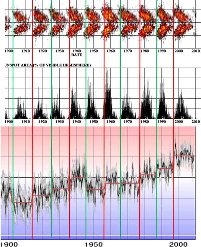
From the figure above it can be seen that the regime changes correspond to the onset of solar cycles and occur when the “butterfly” is at its widest. The most significant warming regime shifts occur at the start of odd-numbered cycles (1937, 1957, 1977, 1997). Each odd-numbered cycle (red lines above) has resulted in a temperature-increase regime shift. Even-numbered cycles (green lines above) have been inconsistent, with some resulting in temperature-decrease regime shifts (1902, 1946) or minor temperature-increase shifts (1926, 1987).
An unusual one is the 1957 – 1966 cycle, which in the monthly data shown above visually looks like a temperature-increase shift in 1957 followed by a temperature-decrease shift in 1964 but the regime detection algorithm did not identify it. This is likely due to the use of annually averaged data in the regime detection algorithm.
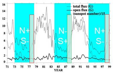
The following figure shows the relative polarity of the Sun’s magnetic poles for recent sunspot cycles along with the solar magnetic flux [www.bu.edu/csp/nas/IHY_MagField.ppt]. The regime change periods are highlighted by the red and green boxes. Each one occurs on as the solar cycle is accelerating. The onset of an odd-numbered sunspot cycle (1977-78, 1997-98) results in the relative alignment of the Earth’s and the Sun’s magnetic fields (positive North pole on the Sun) allowing greater penetration of the geomagnetic storms into the Earth’s atmosphere. “Twenty times more solar particles cross the Earth’s leaky magnetic shield when the sun’s magnetic field is aligned with that of the Earth compared to when the two magnetic fields are oppositely directed” [http://www.nasa.gov/mission_pages/themis/news/themis_leaky_shield.html]
The following figure shows the longitudinally averaged solar magnetic field. This “magnetic butterfly diagram” shows that the sunspots are involved with transporting the field in its reversal. The Earth’s temperature regime shifts are indicated with the superimposed boxes – red on odd numbered solar cycles, green on even.
[http://solarphysics.livingreviews.org/open?pubNo=lrsp-2010-1&page=articlesu8.html]
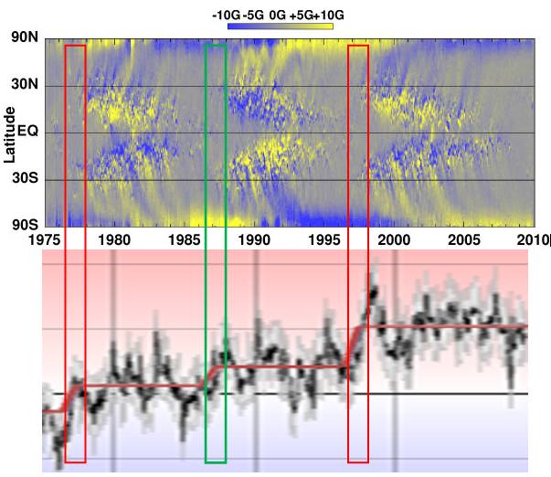
The Earth’s temperature regime shift occurs as the solar magnetic field begins its reversal.
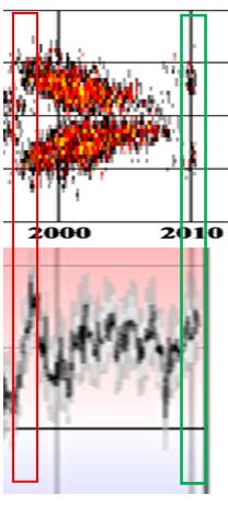
Solar Cycle 24
Solar cycle 24 is in its initial stage after getting off to a late start. An El Nino occurred in the first part of 2010. This may be the start of the next regime shift.
Climate Regime Shifts
[last update: 2010/07/04]
|
“The notion that climate variations often occur in the form of ‘‘regimes’’ began to become appreciated in the 1990s. This paradigm was inspired in large part by the rapid change of the North Pacific climate around 1977 [e.g., Kerr, 1992] and the identification of other abrupt shifts in association with the Pacific Decadal Oscillation (PDO) [Mantua et al., 1997].” [http://www.beringclimate.noaa.gov/regimes/Regime_shift_algorithm.pdf]
|
|
Pacific Regime Shifts
Hare and Mantua, 2000 (“Empirical evidence for North Pacific regime shifts in 1977 and 1989”): “It is now widely accepted that a climatic regime shift transpired in the North Pacific Ocean in the winter of 1976–77. This regime shift has had far reaching consequences for the large marine ecosystems of the North Pacific. Despite the strength and scope of the changes initiated by the shift, it was 10–15 years before it was fully recognized. Subsequent research has suggested that this event was not unique in the historical record but merely the latest in a succession of climatic regime shifts. In this study, we assembled 100 environmental time series, 31 climatic and 69 biological, to determine if there is evidence for common regime signals in the 1965–1997 period of record. Our analysis reproduces previously documented features of the 1977 regime shift, and identifies a further shift in 1989 in some components of the North Pacific ecosystem. The 1989 changes were neither as pervasive as the 1977 changes nor did they signal a simple return to pre-1977 conditions.” [http://www.sciencedirect.com/science?_ob=ArticleURL&_udi=B6V7B-41FTS3S-2…]
Overland et al “North Pacific regime shifts: Definitions, issues and recent transitions” [http://www.pmel.noaa.gov/foci/publications/2008/overN667.pdf]: “climate variables for the North Pacific display shifts near 1977, 1989 and 1998.”
The following figure from the above paper show analysis of PDO and Victoria Index using the Rodionov regime detection algorithm. A regime shift is also detected around 1947-48.
The following figure shows regime shift detection for the summer PDO, showing shifts at 1948, 1976 and 1998. [http://www.beringclimate.noaa.gov/data/Images/PDOs_FigRegime.html]
(For detailed information on the 1976/77 climate shift, see: http://www.appinsys.com/GlobalWarming/The1976-78ClimateShift.htm)
|
|
Regime Shift Detection in Annual Temperature Anomaly Data
The NOAA Bering Climate web site provides the algorithm for regime shift detection developed by Sergei Rodionov [http://www.beringclimate.noaa.gov/regimes/index.html]. The following analyses use the Excel VBA regime change algorithm version 3.2 from this web site.
The following figure shows the regime analysis of the HadCRUT3 annual global annual average temperature anomaly data from the Met Office Hadley Centre for 1895 to 2009 [http://hadobs.metoffice.com/hadcrut3/diagnostics/global/nh+sh/annual].
The analysis was run based on the mean using a significance level of 0.1, cut-off length of 10 and Huber weight parameter of 2 using red noise IP4 subsample size 6. Regime changes are identified in 1902, 1914, 1926, 1937, 1946, 1957, 1977, 1987, and 1997. Running the analysis based on the variance rather than the mean results in regime changes in the bold years listed above.
|
|
Regime Shift Relationship to Solar Cycle
The NASA Solar Physics web site provides the following figure showing sunspot area. [http://solarscience.msfc.nasa.gov/SunspotCycle.shtml]
The following figure compares the Hadley (HadCrut3) monthly global average temperature (from [http://hadobs.metoffice.com/hadcrut3/diagnostics/global/nh+sh/]) overlaid with the regime change line (red line) shown previously, along with the sunspot area since 1900. The sunspot cycle is approximately 11 years. The sun’s magnetic field reverses with each sunspot cycle and thus after two sunspot cycles the magnetic field has completed a cycle – a Hale Cycle – and is back to where it started. Thus a complete magnetic sunspot cycle is approximately 22 years. The figure marks the onset of odd-numbered cycles with a vertical red line, even-numbered cycles with a green line.
From the figure above it can be seen that the regime changes correspond to the onset of solar cycles and occur when the “butterfly” is at its widest. The most significant warming regime shifts occur at the start of odd-numbered cycles (1937, 1957, 1977, 1997). Each odd-numbered cycle (red lines above) has resulted in a temperature-increase regime shift. Even-numbered cycles (green lines above) have been inconsistent, with some resulting in temperature-decrease regime shifts (1902, 1946) or minor temperature-increase shifts (1926, 1987).
An unusual one is the 1957 – 1966 cycle, which in the monthly data shown above visually looks like a temperature-increase shift in 1957 followed by a temperature-decrease shift in 1964 but the regime detection algorithm did not identify it. This is likely due to the use of annually averaged data in the regime detection algorithm.
The following figure shows the relative polarity of the Sun’s magnetic poles for recent sunspot cycles along with the solar magnetic flux [www.bu.edu/csp/nas/IHY_MagField.ppt]. The regime change periods are highlighted by the red and green boxes. Each one occurs on as the solar cycle is accelerating. The onset of an odd-numbered sunspot cycle (1977-78, 1997-98) results in the relative alignment of the Earth’s and the Sun’s magnetic fields (positive North pole on the Sun) allowing greater penetration of the geomagnetic storms into the Earth’s atmosphere. “Twenty times more solar particles cross the Earth’s leaky magnetic shield when the sun’s magnetic field is aligned with that of the Earth compared to when the two magnetic fields are oppositely directed” [http://www.nasa.gov/mission_pages/themis/news/themis_leaky_shield.html]
The following figure shows the longitudinally averaged solar magnetic field. This “magnetic butterfly diagram” shows that the sunspots are involved with transporting the field in its reversal. The Earth’s temperature regime shifts are indicated with the superimposed boxes – red on odd numbered solar cycles, green on even. [http://solarphysics.livingreviews.org/open?pubNo=lrsp-2010-1&page=articlesu8.html]
The Earth’s temperature regime shift occurs as the solar magnetic field begins its reversal.
|
|
Solar Cycle 24
Solar cycle 24 is in its initial stage after getting off to a late start. An El Nino occurred in the first part of 2010. This may be the start of the next regime shift.
|
Stephen Wilde says:
July 8, 2010 at 12:08 pm
Leif, what say you to the top down portion ?
None of the graphs are convincingly different from traditional wisdom, and new data is clouding the picture: http://lasp.colorado.edu/sorce/news/2010ScienceMeeting/doc/Session4/4.04_Cahalan_atmos_model.pdf
I don’t know what to make of it.
tallbloke says:
July 8, 2010 at 3:17 pm
Thanks Leif. I noticed slide 13 showed the 10Be ‘archive’ in the ice would have been affected by precipitation rates, which may have in turn been affected by cloud amounts, affected in turn by the Svensmark effect (putatively). Lots of uncertainty there for me.
There is good [new] evidence that climate effects on both 10Be and 14C are as large or larger than solar activity, so correlating 10Be with temperature, may just be correlating climate with climate.
Bob Tisdale:
Cost isn’t an issue for a blog of my own. Time is, whilst I still have the day job. Anyway I’ll get more out of the comments made on established blogs that attract more and bigger hitters as tallbloke describes them.
That article seems to suggest that the Brewer Dobson circulation is implicated in unexpected vertical energy transport which is what I need so I’ll look into it in more detail.
Observations provide data. The right observations have never been made but I can extrapolate from what we do know.
For example if I am right I would expect to see the strength of El Nino events increase relative to La Nina events the more poleward the air circulation systems go and the strength of La Nina events increase relative to El Nino events the more equatorward the air circulation systems go but I don’t expect to see much on short timescales like a single solar cycle. I think we are stuck with at least the length of the PDV cycle to get any sort of indication.
In the late 70s we had poleward jets and stronger El Ninos than La Ninas. Some expect that we now about to see a period of stronger La Ninas and as it happens the jets are currently more equatorward than they were then.
So when the data is available I can present it and along the way anyone can check it out for themselves.
I’m still waiting for an observation that falsifies my scenario. However I will only accept current or recent evidence. The historical data is far too coarse.
Thank you for suggesting the term Pacific Decadal Variability. Long ago I did say that a new term would be best. If we had thought of it then perhaps that would have been helpful to me and would have made my posts less irritating for you.
That’s as far as we can take the issue here until I’ve checked out the Brewer Dobson aspect and other possible mechanisms for a variable upward energy flux.
I’m sure another relevant thread will come along soon.
Mods, in my previous post please replace ‘late 70s’ with ‘late 20th century’, thanks.
Leif,
http://lasp.colorado.edu/sorce/news/2010ScienceMeeting/doc/Session4/4.04_Cahalan_atmos_model.pdf
Thanks for that further link.
With regard to the chart titled ‘A Contrast In Spectral Variability’ is it correctly labelled on the left ?
Should it read ‘Brightening with INcreasing solar activity’ rather than with DEcreasing solar activity ?
Thanks.
Leif Svalgaard says:
July 8, 2010 at 3:55 pm (Edit)
There is good [new] evidence that climate effects on both 10Be and 14C are as large or larger than solar activity, so correlating 10Be with temperature, may just be correlating climate with climate.
Hmm, maybe. But precipitation rates have been remarkably stable on the centennial scales (as far as we know), though colder generally means drier. I don’t know enough about the chemistry, would 10Be levels in the ice record be affected by the length of time it floated in the atmosphere before being washed down by precip? And since the precip on Antarctica is very low anyway, how much difference would a small change in precip make? I agree that different looking records from different parts of the world speak of terrestrial variation swamping the celestial signal though. Has anyone studied it across a latitudal segment at regular intervals to see if there are other factors causing variation?
I like that one:
Correlating 10Be with temperature, may just be correlating climate with climate.
Stephen Wilde says:
July 8, 2010 at 6:23 pm
With regard to the chart titled ‘A Contrast In Spectral Variability’ is it correctly labelled on the left ?\
Should it read ‘Brightening with INcreasing solar activity’ rather than with DEcreasing solar activity ?
No, it is labelled correctly. That is the big news.
tallbloke says:
July 8, 2010 at 11:39 pm
Hmm, maybe.
No, not maybe.
But precipitation rates have been remarkably stable on the centennial scales (as far as we know)
How do we know?
And we can directly measure the rate for every year simply by how thick the annual layers are.
Has anyone studied it across a latitudal segment at regular intervals to see if there are other factors causing variation?
Ain’t much ice elsewhere except at polar latitudes. And not much need for such a study because the precip is known from the thickness of the layers. Anyway, it is being recognized more and more that climate plays a large role in the 10Be deposition. You see, most of the 10Be is produced at low latitudes [simply because there is much more area down there] and is the transported to the poles, so not only precip is important, also winds and circulation.
vukcevic says:
July 8, 2010 at 11:56 pm
I like that one:
Correlating 10Be with temperature, may just be correlating climate with climate.Correlating 10Be with temperature, may just be correlating climate with climate.
Webber et al. [2010] note in
http://arxiv.org/ftp/arxiv/papers/1004/1004.2675.pdf
“Indeed this implies that more than 50% the 10Be flux increase around, e.g., 1700 A.D., 1810 A.D.and 1895 A.D. is due to non-production related increases! ”
It is rare to see an exclamation mark [!] in a scientific paper.
A very important paper. Thanks for the link.
Perhaps most troubling of all is the cross correlation of the yearly 10Be concentration and
flux measurements themselves from two sites on the polar plateau which should be observing the same 10Be production. These cross correlation coefficients are the lowest of all, less than 0.25 for both concentration and flux measurements and the slopes of the regression lines are less than 0.3.
That is not a good news, lot of papers are based on 10B records. Looks like back to square one. Talking about squares, is their correl coeff R^2 or R; if R then situation is even worse.
Leif Svalgaard says:
July 8, 2010 at 3:55 pm (Edit)
None of the graphs are convincingly different from traditional wisdom, and new data is clouding the picture: http://lasp.colorado.edu/sorce/news/2010ScienceMeeting/doc/Session4/4.04_Cahalan_atmos_model.pdf
I don’t know what to make of it.
The plan at the end looks sensible to me:
Next Steps
Include stratospheric chemistry & circulation (see Haigh, also Stolarski)
Reconsider stratosphere-troposphere coupling mechanisms with alternative forcing
Consider alternative cloud-aerosol feedbacks
Consider alternative forcing scenarios for centennial timescales
Requires coupling to deep ocean
Search for proxies with sensitivity to UV, VIS and NIR multi-decadal trends.
“Stephen Wilde says:
July 8, 2010 at 6:23 pm
With regard to the chart titled ‘A Contrast In Spectral Variability’ is it correctly labelled on the left ?\
Should it read ‘Brightening with INcreasing solar activity’ rather than with DEcreasing solar activity ?
No, it is labelled correctly. That is the big news.”
Well that suits me very well because my observation is that decreasing solar activity sends the polar oscillation negative pushing the clouds equatorward and increasing brightness (albedo) due to the higher angle of incidence of solar energy on to the clouds.
But then what about the other bit below that says “dimming with decreasing solar activity” as against the top part which says “brightening with decreasing solar activity”. The jets go poleward with increased solar activity so brightness should decrease. Thus the lower part should say ‘dimming with increasing solar activity’. One of them must be wrongly labelled unless I’ve misunderstood the chart ?
I’ve seen elsewhere that albedo was dropping during the period of high solar activity but is now rising with the reduced solar activity so my proposition fits that evidence.
vukcevic says:
July 9, 2010 at 1:15 am
is their correl coeff R^2 or R; if R then situation is even worse.
It is R.
Ah, I think I see it. Brightening or dimming depends on the wavelength distribution in the solar spectrum.
More uv leads to brightening and less uv leads to dimming. Thus warming from uv on ozone is offset by increased brightness reflecting visible energy to space and cooling from less uv on ozone is offset by decreased brightness letting more visible energy in.
Please advise whether that is right before I take the next logical step. If I’m wrong please clarify the situation for me and any other confused readers.
Thanks.
Stephen Wilde says:
July 9, 2010 at 6:22 am
More uv leads to brightening and less uv leads to dimming.
No, the UV is not driving this.
The solar cycle is. It is like this: at high solar activity, UV is high, IR is low. At low solar activity UV is low, but IR is high. Visible changes a lot less.
Thus warming from uv on ozone is offset by increased brightness reflecting visible energy to space and cooling from less uv on ozone is offset by decreased brightness letting more visible energy in.
No. That statement is muddled in extreme.
Here is what happens:
High solar activity: more UV [stopped in the stratosphere]. Less IR [which reaches the ground], thus cooling of the surface.
Low solar activity: less UV, but more IR [which reaches the ground], thus heating of the surface.
Leif,
OK, got it now. I’ll work on it and see how it affects my NCM.
My mistake was thinking that brightness was referring to the Earth not the sun. I should have spent more time on it before commenting.
Stephen Wilde says:
July 9, 2010 at 8:06 am
I should have spent more time on it before commenting.
Always a good thing to do… Sage advice.
@AJB says:
July 7, 2010 at 10:16 am
“It rains somewhere every day.”
Some days it rains a great deal in many places, you are welcome to purchase a Weather Action forecast on these highly predictable events.
Stephen Wilde wrote, “Well that suits me very well because my observation is that decreasing solar activity sends the polar oscillation negative pushing the clouds equatorward and increasing brightness (albedo) due to the higher angle of incidence of solar energy on to the clouds.”
A question: Based on your observations, how many degrees latitude are the variations in polar cycles (AO & SAM) pushing the clouds equatorward in response to decreasing solar activity? Say, for example, at No Hem mid-latitudes over the Atlantic and Pacific and the ITCZ over the Atlantic and Pacific. In your NCM post, you use an example of 1000 miles, but how many degrees latitude are you seeing in the aforementioned areas?
@Leif Svalgaard says:
July 9, 2010 at 7:20 am
Stephen Wilde says:
July 9, 2010 at 6:22 am
More uv leads to brightening and less uv leads to dimming.
No, the UV is not driving this.
The solar cycle is. It is like this: at high solar activity, UV is high, IR is low. At low solar activity UV is low, but IR is high. Visible changes a lot less.
Thus warming from uv on ozone is offset by increased brightness reflecting visible energy to space and cooling from less uv on ozone is offset by decreased brightness letting more visible energy in.
No. That statement is muddled in extreme.
Here is what happens:
High solar activity: more UV [stopped in the stratosphere]. Less IR [which reaches the ground], thus cooling of the surface.
Low solar activity: less UV, but more IR [which reaches the ground], thus heating of the surface.
_____________________________________________________
Re. Stephen Wilde; this agrees with the examples I gave you of details of individual spikes in SSN through the solar cycle often being cooler months, and the hot months were at the notches, or lower SSN. So why does the IR vary inverse to UV, and is IR level related to solar wind velocity in particular?
Bob Tisdale asked:
“A question: Based on your observations, how many degrees latitude are the variations in polar cycles (AO & SAM) pushing the clouds equatorward in response to decreasing solar activity? Say, for example, at No Hem mid-latitudes over the Atlantic and Pacific and the ITCZ over the Atlantic and Pacific. In your NCM post, you use an example of 1000 miles, but how many degrees latitude are you seeing in the aforementioned areas?”
Exactly what I would like to know. Where can I find the data ?
There is little doubt that shifts occur over decades and centuries beyond seasonal variation and the movement has been equatorward then poleward then equatorward again during my lifetime (60 years) so who has been keeping an eye on it ?
Just asking those questions puts us both ahead of the pack it seems.
Some AGW proponents attributed the late 20th century poleward shift to human CO2 and suggested it was permanent. Dead silence now.
By the way, have you noticed that Roy Spencer on his website seems to be using the term PDO in the way that you so objected to when I did it ?
Ulric Lyons says:
July 10, 2010 at 3:57 am
So why does the IR vary inverse to UV
That we don’t know, although one can speculate that the high IR is the ‘normal’ situation and if areas that emit UV develop, there will be less area emitting the normal IR.
and is IR level related to solar wind velocity in particular?
No, not likely as the IR level changes are progressing steadily while solar wind speed varies intermittently [in bursts], but we don’t know yet. This data is very new, not even covering a full cycle yet.
I find it interesting [a bit disturbing, actually] that when a new, unexpected [and not yet generally established] result like the in anti-phase varying UV and IR is presented, everybody and his brother immediately claim that this just further confirms and supports their theories…
@Leif Svalgaard says:
July 10, 2010 at 8:27 am
“I find it interesting [a bit disturbing, actually] that when a new, unexpected [and not yet generally established] result like the in anti-phase varying UV and IR is presented, everybody and his brother immediately claim that this just further confirms and supports their theories…”
I had noticed some time back that weekly/monthly SSN change can often be the inverse of temperature changes at this scale, and was suspecting increased IR surface heating at essentially times of higher solar wind velocity, when sunspots are not reducing the coronal holes.
Ulric Lyons says:July 10, 2010 at 3:57 am
So why does the IR vary inverse to UV
In a discharge tube high voltage V is applied to hydrogen, by using Rydberg equation you can calculate emission frequency at different energy levels ( Energy level = Planck’s constant x frequency of light emitted).
At lower V (as far as I remember) electron is still attached to nucleus and will radiate IR, as V increases electron moves up the range of levels, radiation moves from IR towards UV, eventually electron is removed from nucleus.
If the sun has not V available it has other sources of energy.