Guest essay by Joe Born
In Monckton et al., “Why Models Run Hot: Results from an Irreducibly Simple Climate Model,” the manner in which the authors used their so-called transience fraction raised questions in the minds of many readers. The discussion below tells why. It will show that the Monckton et al. paper obscures the various factors that should go into selecting that parameter, and it will suggest that the authors seem to have used it improperly. It will also explain why so many object to their discussion of electronic circuits.
The discussion below will not deal with how well the model performs or whether the Monckton et al. paper interpreted the IPCC reports correctly. It will be limited to basic feedback principles that are obvious to most engineers and to not a few scientists. But there are circumstances in which stating the obvious is helpful, and I believe that Monckton et al. have presented us one.
Equation 1 of the Monckton et al. paper provides us laymen with a handy back-of-the-envelope model by which we can perform sanity checks on things we hear about the climate system. If we concentrate on equilibrium values and assume that carbon dioxide is the only driver, we can drop the  ‘s from that equation’s penultimate line and take the
  and
and  parameters to be unity to obtain:
The expression on the right can be recognized as the solution to the equation illustrated by Fig. 1, namely,  .
.

Here  is a temperature-change response to the initial radiation imbalance
  , or “forcing,” that would result from a carbon-dioxide-concentration-caused optical-density increase. The optical-density increase raises the effective altitude—and, lapse rate being what it is, reduces the effective temperature—from which the earth radiates into space, so less heat escapes, and the earth warms. The
  ‘s represent departures from a hypothetical initial equilibrium state of zero net top-of-the-atmosphere radiation, and the forcing is considered to keep the same value so long as the increased carbon-dioxide concentration does, even if the consequent temperature increase has eliminated the initial radiation imbalance and thus returned the system to equilibrium.
Without any knock-on effects, or “feedback,” the response would simply be  , where
  is a coefficient widely accepted to be approximately 0.32
  . The forcing produced by a carbon-dioxide-concentration increase from
  to
to  is stated by the last line of Monckton et al.’s Equation 1 to be
  , where it is widely accepted that
  , i.e., that a doubling of the CO2 concentration would cause a forcing of about
  .
.
So the model’s user can readily see the significance of the main controversial parameter, namely, the feedback coefficient  , which represents knock-on effects such as those caused by the consequent increases in water vapor, the resultant reduction in lapse rate, etc. In particular, the user can see that if were positive enough to make
  close to unity—i.e., to make the right-hand-side expression’s denominator close to zero—the global temperature would be highly sensitive to small variations in various parameters.
Fig. 2 depicts this effect: approaches infinity as approaches 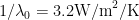 , i.e., as
  approaches unity. (That plot omits
  values that exceed unity; for reasons we discuss below, Monckton et al.’s discussion of that regime in connection with electronic circuits is questionable.)

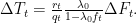
The quantities discussed so far are those that occur at equilibrium, i.e., in the condition that prevails after a given forcing has been constant for a long enough time that transient effects in the response have died out. To arrive at a value for times when the forcing has not been remained unchanged long enough to reach equilibrium, the model includes a “transience fraction” to represent the ratio that the response at time bears to the equilibrium value. Other subscript ‘s are added to indicate that for different times the various quantities’ effective values may differ. Finally, to arrive at the response to all forcings, a coefficient representing the ratio that carbon-dioxide forcing bears to all forcings is included:
As we mentioned above, the transience fraction is of particular interest. As the Monckton et al. paper’s Table 2 shows, the ratio that the response at time bears to its equilibrium value depends not only on time but also on the feedback coefficient . Of course, it would be too complicated for us to investigate how such a dependence arises in the climate models on which the IPCC depends. But we can get an inkling by so modifying the block diagram of Fig. 1 as to incorporate a simple “one-box” (single-pole) time dependence.
Fig. 3 depicts the resultant system. The bottom box bears the legend “ ,” which in some circles means that the rate at which that box’s output changes is the product of its input and a heat capacity
  . (The
  is the complex frequency of which Laplace transforms are functions, but we needn’t deal with that here; suffice it to say that division by in the complex-frequency domain corresponds to integration in the time domain.)
What the diagram says is that a sudden drop in the amount of radiation escaping into space causes the temperature response to rise as the integral of the stimulus divided by . That temperature rise both increases the radiation escape by  and partially offsets that radiation escape by
  .
.

Now, Fig. 3 can justly be criticized for wildly conflating time scales; it does not reflect the fact that the speed with which the surface temperature would respond to optical density alone is much greater than, say, the speed of feedback due to icecap-caused albedo changes. But that diagram is adequate to illustrate certain basic feedback principles.
The output of the Fig. 3 system is a solution to the following equation:

For example, if  equals zero before
  and it equals
  thereafter, that solution for
  is:
is:
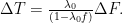
where  . That is, the equilibrium value of
  is the same as it was before we added the time dependence, but the added time dependence shows that the equilibrium value is approached asymptotically.
Fig. 4 depicts the solution for several values of feedback coefficient . What it shows is that a greater feedback coefficient yields a higher temperature output .

Another way of looking at the response is to separate its shape from its amplitude, and that brings us to transience fraction , which is our principal focus. Fig. 5 depicts this quantity, which is the ratio at time of the response to its equilibrium value. That plot shows that, although greater feedback results in a greater equilibrium temperature, it also results in the equilibrium value’s being reached more slowly.

Of course, those plots give the relationship between current and equilibrium output only for our toy, one-box model. Monckton et al. instead employed the relationship set forth in their Table 2 and depicted by the dashed lines in Fig. 6 below. In a manner that their paper does not make entirely clear, they inferred the Table 2 relationship from a paper by Gerard Roe, who explored feedback and depicted in his Fig. 6 (similar to Monckton et al.’s Fig. 4) how a “simple advective-diffusive ocean model” responds to a step in forcing for various values of feedback coefficient.

As Fig. 6 above shows, the Monckton et al. values initially rise more quickly, but then approach unity more slowly, than the ones that result from our Fig. 3 one-box model. As to the specifics of his model, Roe merely referred to a pay-walled paper, but in light of his describing that model as having a “diffusive” aspect we might compare the Table 2 values with the behavior of, say, a semi-infinite slab’s surface, as Fig. 7 does. Except for the  value, the curves are similar over the illustrated time interval, but the slab thermal diffusivity used to generate Fig. 7’s solid curves was about 2000 times that of water, so the nature of the Roe model remains a mystery. Monckton et al. may have had a reason for following Roe’s model choice instead of any other, but they did not share that reason with their readers. For all we can tell, that choice was arbitrary.

More troubling, though, was the fact that they chose only a single transience-fraction curve for each value of total feedback, whereas we would expect that the curve would additionally depend on other factors. Let’s return to a simple lumped-parameter model like Fig. 3 to discuss what some of those factors may be.
Recall that in Fig. 3 the two feedback boxes were the same except for their values and  ; the feedbacks they represent did not operate over different time scales. But the IPCC models can be expected to employ feedbacks that operate with different delays. Feedback effects such as water vapor may act quickly, whereas the albedo effects of melting icecaps may become manifest only over long time intervals.
To illustrate such a difference, we divide the feedback represented by Fig. 3’s upper feedback box into two portions, as Fig. 8 illustrates:  and
and  ,
,  . The legend
  in the uppermost box means that its output asymptotically approaches times the input with a time constant of
  . In other words, if that box’s input were a step from zero to
  at time zero, its output would be
  at time .

Now we’ll compare the responses of Fig. 8-type systems that differ not only in feedback but also in the portion  of the feedback that operates with a greater delay. Fig. 9 compares such different systems’ responses, and we see that, as we expect, the magnitude of the higher-feedback system’s response is greater. In contrast to what we saw before, though, Fig. 10’s comparison of the systems’ curves shows that it is the higher-feedback system that responds more quickly. This tells us that the curve depends not only on the value of total feedback but also on the nature of that feedback’s particular constituents. And it raises the question of what feedback-speed mix Monckton et al. assumed.


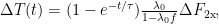
Or maybe it raises the question of just how simple their model is to use. Let’s return to that model and note the dependencies on :
Of the five subscript ’s, three simply represent the time dependence of the stimulus or response, leaving the subscripts on the feedback coefficient  and transience fraction to represent the time dependence of the model itself. That equation might initially suggest a rather complicated relationship: transience fraction depends not only on time but also on the feedback coefficient—which itself depends on time.
But Monckton et al.’s Table 2 suggests that the relationship not quite as convoluted as all that: the transience fraction actually depends not on time-variant feedback but only on  , the value that the feedback coefficient reaches after all feedbacks have completely kicked in. One may therefore speculate that, although the transience-fraction function depends on the feedback’s ultimate value, that function was not intended to account for feedback time variation; one might speculate that the feedback time function serves that purpose.
But that would make the §4.8 discussion of the transience fraction puzzling, since it begins with the observation that “feedbacks act over varying timescales from decades to millennia” and goes on to explain that “the delay in the action of feedbacks and hence in surface temperature response to a given forcing is accounted for by the transience fraction .” So Monckton et al. did not make it clear just where the feedback’s time variation should go. Also, separating the feedback’s final value from its time variation in the manner we just considered doesn’t work out mathematically, particularly in the early years of the stimulus step.
And that brings us to another problem. Note that the forcing used as the stimulus by the Roe paper from which Monckton et al. obtained their Table 2 values was a step function: the forcing took a single step to a new value at and then maintained that value. That’s the type of stimulus we have tacitly assumed in the discussion so far. But the CO2 forcing in real life has been more of a ramp than a step, so we would expect the function to differ from what we have considered previously.
In Fig. 11 the dotted curves represent step and ramp stimuli, while the solid curves represent a common system’s corresponding curves. Obviously, the values are lower for the ramp response than for the step response.

For all that is apparent, though, Monckton et al. failed to make this distinction. In their §7 and Table 4 they appear to use the step-response values of their Table 2 to model the response to a forcing that rose between 1850 and the present, and that forcing was not a step; it was more like a ramp. The Table 2 values could have been used properly, of course, by convolving them with the forcing’s time derivative, but nothing in the Monckton et al. paper suggested employing such an approach—which, in any event, does not lend itself well to pocket-calculator implementation.
Moreover, it’s not clear how Monckton et al.’s §7 statement that “the 0.6 K committed but unrealized warming mentioned in AR4, AR5 is non-existent” was arrived at. That section refers to their Table 4, which shows that the values computed for the model result from multiplication by a transience fraction , supposedly taken from Table 2. The values 0.7, 0.6, and 0.5 respectively given in Table 4 for f values 1, 1.5, 2.2 suggest that in fact the central estimate leaves (1 – 1/0.6) * 0.8 = 0.53 K of warming yet to be realized.
So Monckton et al. have chosen a family of curves based on a model cited by Roe that for all they’ve explained is no better than the toy models of Figs. 3 and 8. Those curves apparently result from applying to that model a step stimulus rather than the more ramp-like stimulus that carbon-dioxide enrichment has caused. Although their discussion did refer to the fact that some feedbacks operate more slowly than others, they did not clearly tell where to incorporate the mix of feedback speeds to be assumed. And, as we just observed, it’s not clear that they properly used the transience-fraction curves they did choose in concluding that “the 0.6 K committed but unrealized warming mentioned in AR4, AR5 is non-existent.” In short, their selection and application of values are confusing.
That doesn’t mean that their model lacks utility. If one keeps in mind that various factors Monckton et al. do not discuss affect the curve, their model can afford insight into various effects that we laymen hear about. In particular, it can help us assess the plausibility of various claimed feedback levels. A particularly effective use of the model is set forth in their §8.1. If the authors’ representation of IPCC feedback estimates is correct, their model helps us laymen appreciate why the IPCC’s failure to reduce its equilibrium climate-sensitivity estimate requires explanation in the face of reduced feedback estimates. And note that §8.1 doesn’t depend on at all.
Despite the confusion caused by Monckton et al.’s discussion of , therefore, Monckton et al. have provided a handy way for us laymen to perform sanity checks. And their model helps us understand their reservations regarding the plausibility of significantly positive feedback. It shows that, generally speaking, one would expect high positive feedback to cause relatively wild swings, whereas the earth’s temperature has remained within a narrow range for hundreds of thousands of years.
Unfortunately, they compromised their argument’s force with an unnecessary discussion of electronics that did more to raise questions than to persuade. Specifically, their paper says:
“In Fig. 5, a regime of temperature stability is represented by  , the maximum value allowed by process engineers designing electronic circuits intended not to oscillate under any operating conditions.”
Although that lore may make sense in some contexts, it’s quite arbitrary; parasitic reactances and other effects can result in unintended oscillation even in amplifiers designed to employ negative values of  . Even worse is the following:
“Also, in electronic circuits, the singularity at  , where the voltage transits from the positive to the negative rail, has a physical meaning: in the climate, it has none.”
And Lord Monckton expanded upon that theme as follows
“Thus, in a circuit, the output (the voltage) becomes negative at loop gains >1.”
Although one can no doubt conjure up a situation in which such a result would eventuate, it’s hardly the inevitable consequence of greater-than-unity loop gains. To see this, consider the circuit of Fig. 12.

The amplifier in that drawing generates an output  that within the amplifier’s normal operating range equals the product of its open-loop gain
  and the difference between signals received at its inverting (-) and non-inverting (+) input ports. In the illustrated circuit the non-inverting input port receives a positive fraction of the output from a resistive voltage-divider network so that, in the absence of the capacitor, the non-inverting port’s input would be
  . A negative voltage at the inverting port would result in a positive output voltage, which, because it is positively fed back, would tend to make the output even more positive than the open-loop value
Now, that is not a particularly typical use of feedback. More typically feedback is designed to be negative because the open-loop gain undesirably depends on the input—i.e., the amplifier is nonlinear—yet for  (and typically is much, much larger than the value 5 we use below for purposes of explanation), the closed-loop gain
 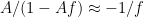 : the relationship
  is nearly linear despite the amplifier’s nonlinearity.
In principle, though, if is independent of input, there are no stray reactances to worry about, we are sure that the feedback coefficient will not change, the lark’s on the wing, etc., etc., then there is no reason why positive feedback cannot be used. If  and
and  , for example, the loop gain
  would be +0.5, which would make the output
  : that feedback would double the gain.
But in that example the loop gain is less than unity. What about  , which makes
  negative? I.e., what about the situation in which Monckton et al. tell us that “in a circuit, the output (the voltage) becomes negative”? Well, despite what they say, it doesn’t necessarily become negative.
To see that, let’s change the feedback coefficient to 0.4 and keep amplifier open-loop gain equal to 5 so that the loop gain  , i.e., so that the loop gain exceeds unity. And let’s make the inverting port’s input
  a time step from 0 volt to -0.1 volt. That value is inverted and amplified, the result appears as the output , and an attenuated version of that output appears at the non-inverting input port.
But propagation from output port to input port is not instantaneous, and, to enable us to observe what may happen during that propagation (and avoid tedious transmission-line math), we have exaggerated the inevitable time delay by placing a capacitor in the feedback circuit. (In a block diagram like those above, the legend on the feedback-circuit block would accordingly be  ).
).
As Fig. 13’s top plot shows, the output is initially (-0.1)(-5) = 0.5 volt and then rises exponentially as the feedback operates. If the amplifier had no limits, the output would grow without bound; despite what Monckton et al. say about in electronic circuits, the output would not go negative.
But we have assumed for Fig. 13 that the amplifier does have limits: its output is limited to less than 15 volts. Accordingly, the output goes no higher than 15 volts even though the signal at the non-inverting input port still increases for a time after the output reaches that limit. Still, the output does not go negative.

We could characterize that effect as the total loop gain’s decreasing to just under unity, as the middle plot illustrates, or as the small-signal loop gain’s falling abruptly to zero, which the bottom plot shows. (That is, no input change that doesn’t raise above +3 volts would result in any output change at all.) No matter how we characterize it, though, the  formula doesn’t apply in this case.
Why? Because it’s the solution to an equation  that says the output is equal to the product of (1) the amplifier gain and (2) the sum of the input
  and a fraction of the output. And in the
  case that equation is never true: delay prevents from ever catching up to
  until the amplifier gain has so decreased that the loop gain no longer exceeds unity.
Now, none of this contradicts Monckton et al.’s main point. Increasingly positive loop gains  make a system more sensitive to variations in parameters such as open-loop gain and feedback coefficient , so in light of the earth’s relatively narrow temperature range it’s unlikely that climate feedbacks are very positive—if they are positive at all. But the authors would have made their point more compellingly if they had avoided the circuit-theory discussion. And they would have made their model more accessible if their discussion of the transience fraction hadn’t raised so many questions.
Like this:
Like Loading...
Discover more from Watts Up With That?
Subscribe to get the latest posts sent to your email.


Wow …. I’m having nightmares of my “circuits” class!! … it’s not a wonder that I just couldn’t stick with Engineering. …. BUT … great presentation.
No kidding! I had flashbacks to early days at U Lowell myself.
I’ve often thought of trying to model the temperature using Electronics Workbench. Input would be TSI, each ocean would represented by a low pass filter, and ocean cycles would be tank circuits, etc. My rational mind, however, tells me that the similarities between global temperature and electronic waveform analysis are superficial. I’m suffering from 30 years of troubleshooting electromagnetic interference issues and my brain is now hard-wired to think in those terms.
Exactly.
I have run simple climate models and making the CO2 input zero makes the model follow reality far better than any other. Kind of makes you think.
Indeed. The key issue with any climate model is to have it model natural climate. If natural climate can be modeled, then the effects if human activity can be sorted out. Current models cannot reproduce the Pleistocene, let alone the changes across the last 550 MY. They cannot reproduce the lag the between increased warming and increased CO2 levels, quite the opposite, they pretty much demand CO2 changes to explain everything else. The short of it is that regardless of how carefully reasoned a model is and how carefully programmed a simulation of the model may be, if that model cannot replicate natural climate at any time scale beyond meteorological models, then it is inadequate. There are missing factors, or factors added that should not be there, or factors to which inappropriate properties have been assigned.
Plus 100…….
Says it all, Max.
…Lambda is a coefficient widely accepted to be approximately 0.32 K/W/m2 …
I don’t know why that is so accepted when it is not the value that the Stefan-Boltzmann (SB) equation predicts (and SB seems to be able to match up energy and temperature everywhere in the universe to nearly 100% accuracy).
For the Surface, SB predicts only 0.184 K/W/m2, and,
For the Tropopause, Earth emitting temperature, SB predicts only 0.265 K/W/m2.
Climate science takes so many shortcuts to keep its theory in the 3.0C per doubling range that they just make up numbers.
I must confess that I have merely accepted that value as being relatively non-controversial; actually going through optical depths for all the different wavelengths is far beyond me, so you’re probably right that I was a little careless in making that assertion.
The optical-density increase raises the effective altitude—and, lapse rate being what it is, reduces the effective temperature—from which the earth radiates into space, so less heat escapes, and the earth warms.
Just what level of atmosphere is being discussed here? Note the inputted energy sources being absorbed by the different layers and until the Thermosphere convection can take place. Has the averaged SB predictions been weighted to the differing temperatures?
http://geogrify.net/GEO1/Images/FOPG/0314.jpg
DD More,
The short answer is: yes, that’s exactly what (spectral) line-by-line radiative transfer codes were designed to do. The atmosphere — not to mention the entire climate system — defies closed-form analytic solutions because it isn’t homgeneous or iso-anything for pretty much any parameter you can think of, so numerical methods (aka – “the models”) are all but necessary.
Mr Illis asks why the Planck parameter at the characteristic-emission level is 0.31 Kelvin per Watt per square meter, when the first differential of the SB equation at that level is 0.27 K/W/m2. The reason for the difference is that allowance must be made for the Hoelder inequality by integrating the individual Stefan-Boltzmann differentials latitude by latitude.
It is interesting, though, that Kevin Trenberth implicitly uses the SB equation at the Earth’s surface in his radiative-balance papers of 1997 and 2008. Strictly speaking, SB does not apply at the Earth’s surface, but only at the locus of all points at or above the surface at which incoming and outgoing radiation are equal.
Kimoto (http://www.ilovemycarbondioxide.com/archives/Kimoto%20paper01.pdf) presents a convincing argument that the real value is around .15 K/W/m^2. He shows where the IPCC and others went wrong and why their calculated values are unphysical. (Note that Kimoto’s lambda = -1/lambda_not where lambda_not is the parameter under discussion.
This was covered in a quite different way (non circuit engineer) at a guest post at CE previously. Not in this detail, but with more climate implications. Go there for additional info.
I commend Mr. Istvan’s piece to readers’ attention. It’s more accessible and boils down the basic feedback concept further, and for some readers reading his piece first would be helpful. But It think something remained to be said about r_t. And then there’s the circuit stuff.
Thanks, Joe Born.
You brought back a lot of electronic circuits theory that I thought I had totally forgotten.
Good post. As I mentioned over at CE not too long ago:
“There is also the bizarre assertion (via misinterpreting a paper from Gerald Roe) that if feedbacks are negative then the Earth system has no thermal inertia and thus transient and equilibrium sensitivity are the same. I’d argue that in its current form the paper should not have been published, and would not have been had it been subject to competent peer review.”
If you look at Roe’s equation 29, its pretty clear that the transience fraction is non-zero for any positive climate sensitivity. Monckton et al’s assumption that the transience fraction is zero when feedbacks are negative is as unjustified as their a-priori assertion of a negative feedback parameter, and certainly disagrees with what Roe says in his paper (which, by the way, is verified via a personal communication with Roe).
I recall your comment and in fact thought that it merited expanding upon.
But by “non-zero” you mean non-unity?
You are correct; I mean that its impossible for r_t to equal 1 if the sensitivity parameter is greater than zero.
Mr Hausfather incorrectly states that Monckton et al. assume that the transience fraction is zero where temperature feedbacks are net-negative. We assume, correctly, that the transience fraction is unity where temperature feedbacks are zero, and that the transience fraction exceeds unity where feedbacks are net-negative, whereas it is <1 where feedbacks are net-positive.
Monckton of Brenchley: “We assume, correctly, that the transience fraction is unity where temperature feedbacks are zero.” value that the corresponding feedback value implies; i.e., to compare the step responses that their Table 2 represents. The result will help assess that statement’s accuracy.
A useful exercise in this context would be to plot on a common graph the product of each row of Monckton et al.’s Table 2 and the
My question – how feasible is it to break out a set of transience functions in an “irreducibly simple model”? How certain could you be of capturing all the different possible physical factors?
Given the claim that the irreducibly simple model does a better job of replicating climate than more more complex models, I think there is a case for lumping transience into a single parameter, until or unless a more sensible breakdown of transience can be constructed in a model which isn’t irreducibly simple, and which does an even better job of reproducing observed climate.
Ability to replicate observation should be the primary objective – if complexity does not help improve replication, it is of no use.
Not sure I quite understand the question, but the following may be relevant. is what I’m told is referred to in some circles as the step response. The only reason I see to break the step response into portions is that seeing the loop gain separately is helpful when you’re trying to understand various features’ effects.
 , the best interpretation is that f should be taken as independent of $t$; to make the math work otherwise requires a feedback-coefficient function that’s highly counter-intuitive.
To the extent that the model is linear–and, despite what the authors say, it basically is linear once the conversion from concentration to radiation is performed–the product of the transience fraction (as inferred from the Roe paper) and
Despite the subscript t on
This false assumption is the real reason Monckton’s “warming but less than we thought” model fails, not feedback flaws. This is essentially the ERL argument, which simply boils down to a claim -”adding radiative gases to the atmosphere will reduce the atmospheres radiative cooling ability”. This claim is clearly ludicrous as the atmosphere would have no radiative cooling ability without these gases.
It becomes doubly ridiculous when the issue of lapse rate is considered. The lapse rate is not a given. It is produced by adiabatic expansion and contraction of air as it vertically circulates across the pressure gradient of the atmosphere. In the troposphere, this vertical circulation depends on radiative subsidence of air masses from altitude. Its speed is therefore dependant on radiative gas concentration. Without radiative subsidence, strong vertical circulation in the Hadley, Ferral and Polar cells would stall, and the bulk of the atmosphere would superheat.
Warmulonians and lukewarmers dodge and weave between “back radiation slowing the cooling of the surface” to ERL and back again. But neither argument holds up.
Given we know current surface average temperatures (288K), the simple way to answer the question – “What is the net effect of our radiatively cooled atmosphere on surface temperatures?” is to correctly answer – “What would the average surface temperature of the planet be without a radiative atmosphere?”.
Because climastrologists got the second question wrong, they can never get the first right. Climastrologists assumed the oceans were a near “blackbody”, and used the Stefan-Boltzmann equation to determine 255K for 240w/m2 of solar insolation. You can’t use the Stefan-Boltzmann equation on SW translucent materials that are IR opaque being intermittently illuminated by solar SW! The oceans are an extreme SW selective surface. They would heat to a surface average around 335K if not for cooling by our radiatively cooled atmosphere.
The climastologists assumption of 255K for “surface without radiative atmosphere” is utterly wrong, and so too is every single paper based on this flawed foundation. 312K is a more accurate estimate. And given current surface temps are lower, this tells you that the net effect of our radiatively cooled atmosphere is surface cooling.
More than anything now, it is the fear and embarrassment of lukewarmers keeping this sorry hoax alive. But trying, as Monckton does, for a Realpolitik “soft landing” can never work. The critical error in the “basic physics” of the “settled science” cannot be erased and no amount of “flappy hands” can change an extreme SW selective surface into a near Blackbody.
Thank you!
Konrad, “The oceans are an extreme SW selective surface. They would heat to a surface average around 335K if not for cooling by our radiatively cooled atmosphere.”
=====================================================
How do you arrive at that number? Are you assuming a non-radiatively cooled atmosphere of equal density?
Konrad says, “The oceans are an extreme SW selective surface. They would heat to a surface average around 335K if not for cooling by our radiatively cooled atmosphere.”
=================================
How did you reach that number.
David A
March 12, 2015 at 11:48 pm
//////////////////////////////////////////////
David,
you ask an intelligent question. First off, the reason you went into moderation and posted twice is because you typed my name. This is a lukewarmer site, therefore my name is treated as the mark of the devil 😉 Evil. Eeeeeevil!
You ask how the 335K number for oceans in the absence of radiatively cooled atmosphere is derived. The simple answer is “empirical experiment”.
I ran a number of these before finding out that the answers had been found by researchers at Texas A&M well before I was even born.
Ultimately an atmosphere without a radiative cooling ability cannot provide surface cooling. Climastrologists never considered this as they assumed that the atmosphere was slowing the cooling rate of the surface.
Try this simple experiment –
http://oi61.tinypic.com/or5rv9.jpg
– both target blocks have the same ability to absorb SW and emit LWIR. Both are opaque to LWIR. The only difference is depth of SW absorption. Illuminate both with 1000w/m2 of LWIR for 3 hours. Both rise to the same average temp. Now try with 1000w/m2 of SW. Now block A runs 20C hotter. Basic physics. Basic physics utterly missing from the “basic physics” of the “settled science”. If you use S-B equations on the oceans you are treating them as SW opaque. My claim that 97% of climastrologists are assclowns is solid.
Wanna try with liquids that convect? –
http://oi62.tinypic.com/zn7a4y.jpg
– ya not gonna win that way either 😉
So what did those researchers who beat me before I was born find –
http://oi62.tinypic.com/1ekg8o.jpg
– for evaporation constrained fresh water solar ponds, layer 2 clear an layer 3 black works far, far better than layer 2 black.
What else did older researchers find? That the deeper evaporation constrained solar pond got, the closer surface Tmin got to surface Tmax. So that’s where the 335K ocean Tav comes from. Empirical experiment shows the sun can drive water to a surface Tmax of 353K or beyond, but due to diurnal cycle, surface Tav will be lower than that.
If in doubt, just remember the five rules governing solar heating of the oceans –
http://i59.tinypic.com/10pdqur.jpg
– the climastrologists didn’t, and that is why they, Willis, Monckton and Spencer failed.
Konrad. March 13, 2015 at 2:11 am
Konrad, I think you meant “that is why they, Willie [Soon], Monckton and Spencer failed”, as I don’t have a dog in this fight.
Regards,
w.
Willis,
I apologise for my lack of clarity. I was indeed referring to you, not the much maligned Dr. Soon.
You claim not to have a dog in this fight. I beg to differ. Remember 2011? Remember what you did at Talkshop? Quite a few real sceptics won’t quickly forget.
You argued that incident LWIR could slow the cooling of water free to evaporatively cool. This is part of the foundation dogma of the church of radiative climastrology. In 2011 I proved that claim false via empirical experiment.
While I appreciate much of your work on the cloud thermostat, the 2011 mistake prevented you from ever finding the correct answer.
If DWLWIR is not heating the oceans above 255K (or at least 273K) as empirical experiment showed it cannot, then some other factors must be responsible for an average of 240w/m2 solar insolation driving the oceans above 255K. I believed my 2011 results, and the results of others who replicated and went searching for those other factors. You did not. This is why you failed.
I found three significant factors. First, hemispherical LWIR emissivity (0.69) for liquid water was far lower than hemispherical SW absorptivity (0.9). Second I found you cannot use apparent emissivity readings for materials (unless very hot) when measured in the Hohlraum of the atmosphere as effective emissivity figures to determine radiative cooling ability. Third, and most important, I found that SB equations don’t work for SW translucent / IR opaque materials being illuminated by solar SW. Water is an extreme SW selective surface, not a near blackbody and it covers 71% of our planet’s surface.
Willis, you and many other lukewarmers are trying to settle for the “warming but less than we though” soft landing. Given warming due to anthropogenic CO2 emissions is a physical impossibility, this is a political dead end. Sceptics have to be right, not just “less wrong”. We have a situation where every single person who is a net negative force toward free market economies and democracy have dug themselves an impossibly deep hole. You are trying to throw them a life line, while I am backing up the JCB to fill the hole in.
You do have a dog in this fight. Problem is this man bites dogs. I only kiss wolves –
http://i57.tinypic.com/2r6p27l.jpg
“But trying, as Monckton does, for a Realpolitik “soft landing” can never work. The critical error in the “basic physics” of the “settled science” cannot be erased and no amount of “flappy hands” can change an extreme SW selective surface into a near Blackbody…”
Good comment and I agree, but I must quibble with the above quote of the last part.
Since there is almost no “science” in modern “climate science” but a whole lot of politics, a “soft landing” might help to get us out of this blind alley that climatology is in right now. I agree that lukewarmers are wrong on parts of the science of the matter, but they are at least challenging the “scientific consensus” and saying that all views should be considered. If we move away from this crazy notion that CO2 is a magic molecule that can do darn near anything, then perhaps we can get back to looking at what the atmosphere really does.
I do agree with you that all the “flappy hands” in the world can not save the current consensus.
Mr Stoval quotes with approval a statement to the effect that the characteristic-emission level is not a near-blackbody. However, with respect to the long-wave radiation in the near infrared that is the object of study, it is a near-blackbody.
Monckton of Brenchley March 14, 2015 at 8:27 am
”Mr Stoval quotes with approval a statement to the effect that the characteristic-emission level is not a near-blackbody. However, with respect to the long-wave radiation in the near infrared that is the object of study, it is a near-blackbody.”
My text Mark quoted referred to the surface of the oceans not the mathematical fiction of a “characteristic emission level”. While water may be opaque to LWIR its surface cannot even be considered a near blackbody in this limited frequency range. First empirical experiment shows incident LWIR cannot heat nor slow the cooling of water that is free to evaporatively cool. Second the hemispherical emissivity of water in the LWIR is only around 0.67.
I understand the desire of lukewarmers to flee from discussion of surface properties of the oceans with regard to absorption and emission of radiation, as this is where the critical error that invalidates the entire radiative GHE hypothesis lays. However running to the old ERL or “characteristic emission level” game is no solution. Anyone with an IR thermometer can see for themselves that the 5km claims are false.
Remember what Sir George Simpson of the royal meteorological society warned Callendar in 1939 –
“..but he would like to mention a few points which Mr. Callendar might wish to reconsider. In the first place he thought it was not sufficiently realised by non-meteorologists who came for the first time to help the Society in its study, that it was impossible to solve the problem of the temperature distribution in the atmosphere by working out the radiation. The atmosphere was not in a state of radiative equilibrium, and it also received heat by transfer from one part to another. In the second place, one had to remember that the temperature distribution in the atmosphere was determined almost entirely by the movement of the air up and down. This forced the atmosphere into a temperature distribution which was quite out of balance with the radiation. One could not, therefore, calculate the effect of changing any one factor in the atmosphere..”
Konrad’s comment is solid. For those not familiar with radiative transfer theory, hopefully here is a simplified, easy to imagine version. Imagine a molecule adsorbing energy from solar radiation. This extra energy in the molecule puts the molecule in an excited state which it doesn’t “like”. There are a number of ways the molecule can get rid of the extra energy, such as direct transfer to another molecule or by the emission of electromagnetic photon(s). This latter way is described as radiative transfer and usually the newly emitted photon is at specific wavelengths/frequencies which are likely to be adsorbed by other molecules. Let’s say a CO2 molecule sheds its excess energy near ground level, this energy will likely be absorbed by other molecules – either in the air or in the earth (water, soil, etc.). Additionally the photons can go in any direction – up, down, sideways. The conservation of energy continues in this fashion.
There are basically two ways the photon energy can be lost to space;
1) The photon is of a wavelength/frequency to which intervening molecules (air) are transparent. Molecules normally only adsorb specific w/f’s in the electron shell, which is the bulk of an atom’s size. If the w/f is not specifically adsorbed in the electron shell, then it will pass right on through. Any w/f normally can be adsorbed by a nucleus, but there is less of a chance of this due to the nucleus’ relatively small size compared to the total size of the atom.
2) The energized molecule is close to outer space with little intervening and adsorptive molecules between the photon and space. Additionally, the photon must be travelling towards space (not down towards earth). This is where Konrad’s comments are so important. An excited CO2 molecule WILL lose its excess energy eventually, sometimes right away, other times after a period of holding the energy. There is a good chance other molecules, e.g. water, will adsorb the CO2’s excess energy. Now excited, all these atmospheric molecules will also release their excess energy in good time. Where that energy goes partially depends on where the molecule is at the time of the energy release. Near the Earth’s surface, the energy will more than likely be retained in the Earth’s environment. But if the excited molecule is transported to the upper atmosphere as Konrad is saying, it could release its energy to space.
There are other ways photon energy can be used instead of becoming molecular excitation (which can translate to what we call heat). For example, the photon adsorption may cause the breaking of chemical bonds. This happens a lot in our atmosphere. Whether or not this is exothermic (heat releasing) depends on the reaction. In short, there is no way we can calculate all the possible perturbations of radiative transfer in the atmosphere’s chaotic system. We can come up with fudge factors that take this into account, but from all the things I’ve seen on WUWT, those fudge factors are all over the spectrum.
I don’t know if we are in the beginning of our learning process or whether we are in the middle of it, but I can confidently predict that we are a very long ways from having a true understanding. To rely on any climate theory at this time is foolish hubris.
Thank you for a nice comment. Couple of remarks: Regarding CO2, it is almost never excited by solar radiation. It is much more likely to be excited by an infrared photon from the surface or the atmosphere. Your point 1 is essentially correct, except that nuclei don’t need to be mentioned at all (if you do, please provide a correct explanation). Your point 2 mixes two concepts: an emission of a photon (correct) and other ways to dispose of the excitation energy. Here you omit a basic mechanism: an excited molecule (in a rotational or vibrational state) may collide with another molecule, most likely a N2, and the energy will be converted to a kinetic energy – heat.
K*nrad, got a link for the Texas A&M research?
beng1, I’m sure he does, the question is will he provide it. Not that it makes much difference: sunlight penetration in the oceans is much studied, a quick search should turn up multiple hits all saying what K-rad is, none of it mysterious, controversial, or being ignored by “climastrologers”. That isn’t where his argument breaks, but at the very least he’s got a sense of humor about it: “shredded turkey in Boltzmannic vinegar” gave me a case of giggleshits.
Beng,
the 1965 work I refer to is –
Harris, W. B., Davison, R. R., and Hood, D. W. (1965) ‘Design and operating characteristics of an experimental solar water heater’ Solar Energy, 9(4), pp. 193-196.
– sadly I do not have a link to an non-paywalled copy online.
However you will find it referenced in a few places including Ibrahim Alenezi’s 2012 thesis on salt gradient solar ponds where he writes –
“A group of researchers at Texas A&M University [20] tried to improve the SSP by using a completely black butyl rubber bag. However, the result was exactly the opposite of what they had tried to achieve: the temperature of the top surface of the bag was 30oC hotter than the water directly underneath. So, the conclusion confirmed that the upper cover should be a transparent film.”
Harris et. al. were experimenting with shallow freshwater solar ponds. Because evaporation constrained freshwater solar ponds have no barrier to convection, they suffer from overnight surface cooling. The solutions were all too costly – insulated night covers, pumping to insulated night storage tanks or making the ponds very deep (remember sunlight penetrates our oceans to 200m). Because of the impracticalities of freshwater ponds, salt gradient with its convective constraints became the favoured technology. The physics pertaining to freshwater evaporation constrained ponds however remains relevant to how the sun heats our deep transparent oceans. Ie: DWLWIR need not be invoked to keep the oceans from freezing.
Brandon Gates
March 13, 2015 at 2:20 pm
/////////////////////////////////////////////////
A “quick search” was it darling? So where are your results showing climastrologists actually had the brain to treat the oceans as an extreme SW selective surface? Nowhere, that’s where! All of their calculation are based on assuming the surface of our ocean planet is a “near blackbody”. This is what is so delightful sweetheart. You and yours are trapped by the Internet. You fecukd up something severe, and you can never erase your shame.
Is it just the “happy few” sceptics who fought on St. Crispins day coming after you? Hell no! You and yours pissed the engineers off. Way stupid move. You could convince the activists, journalists and politicians of the Left. But white coats and no empirical evidence don’t work on engineers. Engineers outnumber all your people, but you thought it a good idea to piss up our backs and tell us it was raining. You’re gonna pay!
Tell engineers they are “holocaust deniers” for pointing out flaws in your failed hypothesis, they don’t back down. They get pissed off. The eyes narrow and a wind of rage flips the desk calender to weasel stomping day –
Brandon, sweetheart, pet, love, let me tell you what happens next. You won’t be just up against a few hundred thousand sceptics. You will be up against the general public. Billions of them. Billions of enraged citizens, baying for political blood. Did you foolishly think each of the warmulonian transgressions were lost in the dust of battle? Think again! Engineers are good at building dams, and we have recorded ever single inanity the warmulonians have ever uttered. Will the dam burst and allow any of yours to escape in the confusion? Forget that.
Sceptics maintain the dam of anger, but we will give control of the small valve at the base to the general public. Turn that valve and you release an iron hard jet of rage that will power the turbines of vengeance.
(This comment is my homage to the recently late Terry Practchett. I accept his choices, but still regret his passing.)
Konrad,
Clayton and Simpson (1975), “Irradiance Measurements in the Upper Ocean”: http://journals.ametsoc.org/doi/abs/10.1175/1520-0485%281977%29007%3C0952:IMITUO%3E2.0.CO;2
Abstract
Observations were made of downward solar radiation as a function of depth during an experiment in the North Pacific (35°N, 155°W). The irradiance meter employed was sensitive to solar radiation of wavelength 400–1000 nm arriving from above at a horizontal surface. Because of selective absorption of the short and long wavelengths, the irradiance decreases much faster than exponential in the upper few meters, falling to one-third of the incident value between 2 and 3 m depth. Below 10 m the decrease was exponential at a rate characteristic of moderately clear water of Type IA.
Gasparovic and Tubbs (1975), “Influence of reference source properties on ocean heat flux determination with two-Wavelength radiometry”: http://onlinelibrary.wiley.com/doi/10.1029/JC080i018p02667/abstract
Abstract
Multiwavelength infrared radiometers used for determining the heat flux through the ocean surface are generally calibrated by using a near-ambient temperature reference radiation source. Typically these sources have spectral emissivities that are less than unity and wavelength dependent. Analysis of the error produced by using a reference source which only approximates an ideal blackbody indicates that significant errors in the heat flux determination can arise unless the emissive properties of the source are well-known and accounted for.
Goldberg (1961), “Radiation from Planet Earth”: http://oai.dtic.mil/oai/oai?verb=getRecord&metadataPrefix=html&identifier=AD0266790
Abstract : Information is given on the part played by the sun, earth’s surface, and atmosphere in the heat balance of our planet. Following a general survey of solar and terrestrial radiation, including the emissivity and reflectivity of various terrestrial features (clouds, land masses, oceans), an estimate is made of the planetary radiation received by a satellite radiometer in five spectral channels covering the ultraviolet, visible, and infrared spectral regions. The wavelengths and purpose for selecting each of the channels is given. The signal-to-noise ratios associated with the received radiation in each channel using bolometers such as those in TIROS II and III, are included.
Saunders (1967): http://journals.ametsoc.org/doi/abs/10.1175/1520-0469%281967%29024%3C0269:TTATOA%3E2.0.CO;2
A simple theory is presented to account for the difference between the temperature at the ocean-air interface and that of the water at a depth of about one meter. Except in very light winds and intense solar radiation the mean temperature difference ΔT is expected to be of the form [of a bunch of symbols I don’t feel like representing in Unicode] where q is the sum of the sensible, latent, and long-wave radiative heat flux from ocean to atmosphere and τ/ρw is the kinematic stress. No data are available to test this prediction.
The influence of slicks and solar insolation on interface temperature is also briefly discussed.
Not in ’67 anyway, but it’s a heavily cited paper, including three this year already. Sort of a must-read, actually, because it’s an accessible yet comprehensive overview of all of the fluxes contributing to near-surface ocean temperatures.
That really should be enough. That emissivity isn’t constant over all wavelengths any more than albedo is constant for all surfaces at all times is pretty much common knowledge at this point … which may explain why it’s not explicity discussed in more recent literature.
Idiocy or pathological lies. So hard to tell sometimes.
No. Start with Hansen and Lacis (1973), “A Parameterization for the Absorption of Solar Radiation in the Earth’s Atmosphere” (open-access): http://journals.ametsoc.org/doi/abs/10.1175/1520-0469%281974%29031%3C0118:APFTAO%3E2.0.CO;2
Please point to the text which says, “we assume the entire surface is a ‘near blackbody'”.
Maybe you’re thinking about papers like this: Wetherald and Manabe(1975), “The Effects of Changing the Solar Constant on the Climate of a General Circulation Model”http://journals.ametsoc.org/doi/abs/10.1175/1520-0469%281975%29032%3C2044:TEOCTS%3E2.0.CO;2
A study is conducted to evaluate the response of a simplified three-dimensional model climate to changes of the solar constant. The model explicitly computes the heat transport by large-scale atmospheric disturbances. It contains the following simplifications: a limited computational domain, an idealized topography, no heat transport by ocean currents, no seasonal variation, and fixed cloudiness.
And then leads off with, “A very crude estimate of the sensitivity of the equilibrium temperature of the atmosphere to the change in solar constant may be obtained from the equation …”, a fancied up version of S-B, which when one assumes an average planetary albedo of 0.3, like textbooks often do, results in a 1% change in solar constant spitting out a 0.6 °C change in equilibrium temperature.
Just because one can find simplifications in literature does not mean that everyone, everywhere, all the time, is using the back of envelope approximations when they’ve got the accuracy requirements AND computational horsepower to do heavier lifting.
You’re going to apologize for being a reality-impaired fruitloop and seek help? No, of course not. Smooches dear one, you were fun as always.
Brandon,
nice try but no cigar. Why didn’t you settle for Sweeney et al? It reads sooo much better. A tiny oceanographers voice in the wilderness calling to the climastrologists “Guys? Um err, guys?”
”Please point to the text which says, “we assume the entire surface is a ‘near blackbody’”. “
Bwahahahaha –
No Brandon, there is no way out. “Surface in absence of atmosphere at 255K being raised by 33K by addition of a radiative atmosphere” is just too wide spread for you ever to erase it. This claim is in every basic Gorebull warbling text. The shame of the climastorlogists will burn forever 😉
”You’re going to apologize for being a reality-impaired fruitloop and seek help”
Now why on earth would I do that Brandon? I was never so inane as to claim that adding radiative gases to the atmosphere would reduce its radiative cooling ability. You and yours own that one darl’ 😉
Konrad,
I don’t know that paper, sounds interesting. Hit me.
Moving the goalposts. Your claim was that climastrologists ignore the selective absorptivity/emissivity of the oceans. That claim is false.
I’ve already stipulated that the problem is simplified in texts. A first year physics student solves ballistic trajectory problems neglecting the planet’s rotation and atmosphere entirely. If they go on to design harware like this …
http://en.wikipedia.org/wiki/File:M3-M4_gun_computer.jpg
… for the military, then they must draw from higher level coursework and take air temperature, humidity, wind speed, drag coefficient, Coriolis and Magnus effect and a slew of other things into account. Every engineer was a first year physics student at one point, doing vastly oversimplified calculations. Including YOU. Throw yourself under the bus, netl00n.
I really shouldn’t have to invoke Kirchhoff, but a radiative atmosphere is also an absorbing atmosphere.
http://photonics.intec.ugent.be/education/ivpv/res_handbook/v1ch44.pdf
It gets good right around the discussion of Beer-Lambert on p. 10. Twit. Hugs ‘n kisses.
Brandon Gates March 15, 2015 at 3:11 pm
”Moving the goalposts. Your claim was that climastrologists ignore the selective absorptivity/emissivity of the oceans. That claim is false.”
Oh Please, Brandon there is no way out. This is not about insignificant errors, this is about a 60K error in the “basic physics” of the “settled science”. Try moving the goal posts all you like. Warmulonians are good at that. One of my speciality areas is thermite plasma FAE. Blast radius 5km. 300 psi overpresure at 3 km. You can’t run fast enough 😉
”I’ve already stipulated that the problem is simplified in texts.”
Simplified was it darl’? No, no “out” there. You and yours claimed that the net effect of our radiative atmosphere was surface warming, not surface cooling. This is black or white, right or wrong. There is no room for “nuance”
You say I throw myself under a bus? Dream on. No one would even dare push me. They can’t crack the butterfly wing encryption!
Sure I’m a monster, but I’m the monster you deserve.
Konrad,
Which you attempted to address by saying that the ocean’s extreme SW selectivity has been ignored. That is false. You mention Sweeney, et. al by way of rebuttal, and failed to produce a citation when asked. Did you mean this paper? Sweeney, et al. (2004), “Impacts of Shortwave Penetration Depth on Large-Scale Ocean Circulation and Heat Transport” http://journals.ametsoc.org/doi/pdf/10.1175/JPO2740.1
Perhaps not, since it’s yet more evidence that climastrologists aren’t ignoring that which you say they are. So now you’re down to argument by assertion and indulging yourself with fantasies of rupturing my internals with thermobaric ordnances. Charming, my pet, quite charming.
Kirchoff, Beer and Lambert — the arch-climastrologists.
The planet is not your lab bench, my silly sweet. True/false dichotomies are difficult to come by, but some things can still be tested in controlled conditions. And have been. Rubens and Aschkinass (1898), “Observations on the Absorption and Emission of Aqueous Vapor and Carbon Dioxide in the Infra-Red Spectrum”: http://adsabs.harvard.edu/abs/1898ApJ…..8..176R
The absorption band at 14.7μ is so sharp that it comes out distinctly in every energy curve in consequence of the carbon dioxide in the air of the room, while the absorption bands of water vapor cannot be observed this way under an average humidity.
The observations now communicated show that the Earth’s atmosphere must be wholly opaque for rays of wave-length 12μ to 20μ as well as for those of wave-length 24.4μ.
This kind of stuff has been done so often and is now so routine that it’s an undergrad-level lab exercise: http://www.d.umn.edu/~psiders/courses/chem4644/labinstructions/COIR.pdf
At the surface, CO2 absorbs so strongly in the 15μm that transmittance falls to practically ZERO for path lengths on the order of tens of meters. In English, that means that if our eyes were only sensitive to frequencies in the 14-16μm region of the spectrum, at the surface of this planet the scatter from CO2 in this band would be akin to what a thick fog does for us in the real world at the frequencies our eyes actually do detect naturally. From space, for satellites which can “see” 15μm radiation, the results are pretty striking:
The only reason that weather birds can see anything at 14-16μm is because that’s in a sweet spot for CO2 emissivity. That’s Kirchoff. However, by Beer-Lambert — and via lab observation — we know the satellites can only be seeing that radiation from the upper layers of the atmosphere. This is corroborated by the radiance in those bands dipping down to almost 210 K as would be predicted by the Stefan-Boltzman relationship.
Konrad attributes to me a false assumption that is not made in Monckton et al., but it is made by Mr Born. Effective temperature does not change as a consequence of a change in the mean altitude of the characteristic-emission level.
Monckton of Brenchley
March 14, 2015 at 8:24 am
”Konrad attributes to me a false assumption that is not made in Monckton et al., but it is made by Mr Born. Effective temperature does not change as a consequence of a change in the mean altitude of the characteristic-emission level.”
Viscount Monckton,
I agree that Joe Born’s text I quoted is more a description of the old ERL argument rather than the “characteristic emission height” variant you use in your paper. The problem is that the same flaws in reasoning apply to both. It is just as Sir George Simpson said to Callendar in 1939 – “it was impossible to solve the problem of the temperature distribution in the atmosphere by working out the radiation.”
The 5 km you use is a mathematical assumption and not supported by empirical observation. Get an IR instrument and measure the sky. Clouds are the strongest emitters. Clouds emit most strongly at low altitude, and very strongly during formation due to the heat pulse during the release of latent heat. Trying to calculate a “characteristic emission height” from IR opacity maths games defies reason.
If empirical experiment is not your thing then see others observations of the net energy fluxes into and out of our gas atmosphere. Absorption of LWIR surface radiation accounts for less than 33% of all energy entering the atmosphere. Emission of LWIR to space however accounts for almost 100% energy leaving the atmosphere. So the net effect of radiative gases in our atmosphere both absorbing and emitting LWIR is atmospheric cooling.
Could such a radiative cooled atmosphere be warming the surface of the planet? No, as empirical experiment shows, the oceans would rise to 335K or beyond were it not for atmospheric cooling. A non-radiative atmosphere could not cool the oceans as it would have no effective way to cool itself.
There truly is no point to the “warming but less than we thought” games. Given there is no net radiative GHE on this planet, the Realpolitik approach is a dead end.
Nice presentation and critique of probably all models in the climate quiver. I have problems with the entire subject of these models. I have problems with time periods for forced temperatures going several centuries. A cooling period of sufficient length, say one as long as the 20yr warming period we are to be alarmed about, would presumably have multi century long feedbacks that would continue to cool. Indeed, such a thing as polar amplification becomes polar de-amplification and all those rising curves become descending curves. Imagine sliding down into the LIA. Can we say that we still have feedbacks that are still descending from that? More. We had a Medieval Warm Period (I continue to use this venerable term) that would have sent more warming down the pipeline that got lost in a cooling period. Climate optimum 7000yrs ago followed by cooling followed by Minoan Warm Period, followed by cooling, followed by Roman WP:, Dark Ages Cool period, Medieval….. These things were all happening (allegedly) with CO2 below 300ppmv with possibly even greater amplitudes. These also are the wiggles that are on the big oscillations of 100,000, 20,000 and 40,000yrs with amplitudes of ~4-5C that occur whether CO2 is 7000ppm to 280ppm warm or cold. This is the natural variation that any anthropo forcing has to overcome and it could come in handy if we could do so, let’s hope.
In summary, my problem with Monckton et al is they may have a model that performs better than others but there is little likelihood it approximates reality. This has been my nightmare: what if these people that want an new world order to subject the free had accidentally hit upon a model that, although it had nothing to do with reality, accidentally predicted future temperatures up to now. They would be shutting down fossil fuels and accidentally coinciding with the hiatus that’s upon us and taking credit for saving the planet. Our willing governments would already be taxing and expropriating and impoverishing us to subsistence if we were lucky, in preparation for the next dark ages. There is a plot for Hollywood. Good, I got that rant out of my system
Gary, guess what? They already have a general circulation model that is the stuff of your nightmares: the Quantity Theory of Money and its paraphernalia. Because of this model, we are repeating the worst mistakes of history. Few realize that the Western half of the Roman empire collapsed because currency debasement caused gold to go into hiding, and the Dark Ages followed in its wake. The Eastern half avoided currency debasement by keeping its mints open to gold coinage — the gold Bezant — and as a consequence, flourished for another thousand years. We are copying the West, not the East.
See: GOLD IN HOARDS versus GOLD ON THE GO: Splitting the Roman Empire into two halves
Also see: Wikipedia > Gold Bezant
As a friend of mine would playfully put it: Wake up Cinderella, your pumpkin is here!
The primary reason for the dark ages had nothing to do with money, the reason civilization regressed was the earth cooled, the roman warm period ended. Cool is bad warm is good, if only people understood this, cold crops fail, warm you can grow more crops. The same for increased CO2. I use to think the collective intelligence of the human race was postie, the global warming debate makes me thing the it is negative. If it is negative God help us all.
Mark,
Of course it had nothing to do with the Huns, Visigoths, empires expanding at others demise..
Gold has no more intrinsic value than other currencies — only what we (or “the market”) give it . One form of price manipulation merely replaces another. But that doesn’t mean you can’t make a profit off the fluctuations of either commodity.
About the Huns: the invention of the stirrup came from Central Asia and suddenly a huge number of horse riding warriors appeared out of nowhere and they dominated warfare for the following 2,000 years.
It should be clear by now that what is being “modeled” is far more ideological than scientific. I prove my theory by noting that the output of almost every single climate model is a model of government action that all converge on larger government, more regulation, higher taxation, subsidies of favored parties and far less personal freedom.
The contra-proof is what these advocates are not interested in knowing: there seems to be no appetite for knowing the ideal climate for our current biosphere and where is our climate in comparison to it.
Best post i have read in weeks. Dead on.
As the preponderance of evidence grows with regard to the principle of reasonable doubt, the Arrhenius Hypothesis IS fail.
I’ve always said that it isn’t worth even trying to model a chaotic system like the climate. The money and time could have been far better spent on something else.
Amen, Trying to model something you don’t understand will always fail, trying to predict the future will always fail. Thinking a computer will make such models and\or predictions any better is the height of stupidity.
Modelling on a false premise will always end up with the wrong answer, regardless of the model.
A computer will only get you to the wrong answer faster
Not entirely. I have recently been looking at the scale of variability of the climate over various periods. From this I can predict what will happen – or at least the upper and lower limits of what is typical given past behaviour. From this I can start to make some tentative statements about whether warming or cooling is most likely in the next few decades and how much that is likely to be on average.
Quite agree. In the last 20 years, literally just in the USA, billions of US dollars have been spent on climate models, super computer time, meetings, salaries, more meetings, to achieve a politically desired output. Dr Collin’s specious claims in the story down thread on WUWT is vivid evidence of his deep seated desire to maintain the aCO2 AGW scam.
The simple fact is that very simple models are no more skilful at predicting the climate than massive supercomputers. This is not welcome news to a whole group of people who earn their living through massively complex models and supercomputers.
All you need to know is that we are much closer to the top of the historical temperature range then we are the bottom and it is still just barely warm enough.
Joe –
Can you explain why you chose the particular circuit of Fig. 12? I take the amplifier A to be a finite-gain (A) differential input, with no frequency compensation (that is, not like a real op-amp). This assumed the network with feedback is just a negative real pole with a real zero slightly further back (more negative). It is a quite trivial to analyze the transient (like step response) and the steady-state (frequency) responses. Did you look at these plots and do they MEAN anything?
I chose those simplified, idealized assumptions to make the circuit straightforward to understand; the only “complication” was the capacitor used to provide a delay that could be easily analyzed.
For the simplified, idealized values shown, the step response is as you see, but I would have said that the (real) zero is less, rather than more, negative. Be that as it may, the post was dry enough without venturing into poles and zeros.
I didn’t do a steady-state analysis, because it wasn’t germane. Moreover, I think Lord Monckton’s difficulty arises from his having spoken with engineers, who, in my experience, tend to speak about complex-number feedback values, i.e., steady-state-analysis values, and that can lead to false conclusions if you don’t really think through what those values mean. And the capacitor, which is all that results in a frequency dependence, was merely a way of using a delay whose math even a retired lawyer such as I could manage.
The only point of that circuit analysis was to show that greater-than-unity loop gain does not have the meaning that Lord Monckton seems to have attributed to it. When engineers have objected to that meaning, they haven’t broken the analysis down well enough for him to take their meaning. I probably haven’t, either, but I thought I’d make the attempt.
While I dislike Monckton’s circuit language, I think you’ve played some word smithing games as well. Monckton stated (correctly) that the output voltage of his feedback circuit will go negative. He’s correct because he’s increasing voltage(temperature) and the circuit both you and he use inverts the output. You chose to inject a negative signal and –surprise!– it inverts just like it’s supposed to. Sure, it doesn’t always “go negative” but I don’t think that was really his general point but the specific signs for the specific problem at hand.
That said there was nothing technically wrong with any of your derivations and his use of feedback terminology was sloppy but correct with his assumptions.
Tsk Tsk: “I think you’ve played some word smithing games as well.”
I don’t think so. In retrospect I would have been better advised not to have used a differential amplifier–i.e., not to have applied the input to an inverting port–but the effect would have been the same if I had made both ports non-inverting.
Let’s change the system so that both ports are non-inverting, and let’s make the input a positive step. Under less-than-unity loop gain, the output asymptotically increases to a finite positive multiple of the input so long as that doesn’t exceed amplifier limits, but in any case it doesn’t turn negative. Under greater-than-unity loop gain, on the other hand, the output increase without limit–until it reaches the amplifier’s limit–and, again, it doesn’t go negative.
Again, there is a sense in which the negative values in the lower right portion of Monckton et al.’s Fig. 5 do have meaning. But the meaning isn’t necessarily that the output “transits to the negative rail.” And to me it’s far from clear that its meaning distinguishes electric circuits from the climate as modeled by Monckton et al.
Oops! You were right about the zero being more negative.
Thanks Joe!
Your treatise reminded my why I chose metallurgical engineering over electrical engineering!
Mac
Complex equations based on false assumptions will still give wrong answers. Eliminate the “back radiation”, “radiative forcing”, “feedback loops”, etc before attempting to model the climate. Until climatologists do they will continue to get correct answers for their sums but be constantly surprised by reality giving different answers.
Thanks Anthony.
A good laugh is always worth putting up.
Mr Born’s impressive amount of writing on nothing is very informative. As has been his comments at Lucia’s and Curry’s.
I am glad you read it and understood it well enough to put it up as a serious article.
He has an issue with Monckton, tough luck.
He has an issue with a lot of things, ditto.
Monckton et al put up a simple example of why global warming is over hyped.
I get that.
Someone comes along and nit picks that he has found a flaw in the example.
Spends 5 pages talking about other things then raises the obscure and irrelevant focus of his ire.
which has nothing to do with a simple example.
We are treated to pages of impressive sounding but unexplained gobbledygook and then told that in some rare cases only Joe can find the example might not hold.
Zeke Hausfather said
” its pretty clear that the transience fraction is non-zero for any positive climate sensitivity. Monckton et al’s assumption that the transience fraction is zero when feedbacks are negative is as unjustified as their a-priori assertion of a negative feedback parameter,”
Only comments are “pretty clear” is funny terminology for “bleeding obvious” but does not mean he is right re Monckton’s assumption of transience fraction being zero when feedbacks are negative.
What Monckton meant is that if negative feedbacks are large enough the transience fraction is indistinguishable from zero, ie practically zero.
It is obvious that Joe and Zeke do not know what the word “practical” means.
It means commonsense.
,i>”Monckton et al put up a simple example of why global warming is over hyped.
I get that.”
No, what Viscount Monckton put up was a pathetic variant of the ERL argument. He is of course wrong. AGW due to CO2 is a physical impossibility. I mean seriously? He is arguing that adding radiative gases to the atmosphere will reduce our radiatively cooled atmosphere’s ability to cool the surface of our solar heated oceans. Utter drivel!
Monckton is a mathematician. He has a 2D brain. There is no way he can solve for “x” if the answer requires 3D CFD. To set up a CFD run you need a 3D brain. You need an engineer.
Global warming was in effect a global IQ test, with results permanently recorded on the Internet. For all his help to the sceptic community, Monckton still failed. Sadly the reason was ego. He bought the “1.2C warming for a doubling of CO2” thing, and refused to back down.
At this point, Viscount Monckton has become a liability to sceptics, not an asset. The same goes for Willis. When empirical empirical experiment proved both wrong, they both ran to gatekeeping to protect their own hides. They both committed the same sin as the climastrologists.
Don’t get me wrong, I have paid to see Viscount Monckton talk when he was on tour several times. I have admired his efforts. But his “warming, but less than we thought” offerings, especially after he has been shown the right answer, disgust me. In the end he acted just like the warmulonians, and the reason is inexcusable – Ego.
I think you’ve nailed it there………a lot of the argument has become them against us. Whatever his intentions Monckton is a bit of a pantomime act – if you wanted to be taken seriously you wouldn’t want to wheel him out on your side.
Yah-boo has no place in ths thread.
Viscount Monckton,
“Yah-Boo” would imply that I have a knee jerk response to deride or disagree with everything you assert. This is not the case. Up thread you state – “Strictly speaking, SB does not apply at the Earth’s surface.”
I totally agree with this statement, and I have posted the empirical experiments on this thread that prove it wholly correct. I am having a jab at you (mild in comparison to the previous thread on your model) because you are ignoring the implications of that statement.
When it comes to determining the effect of our radiative atmosphere on surface temperatures, understanding surface properties is the KEY. After all, the surface is the primary point of solar energy input into the land/ocean/atmospheric system.
In comparison, establishing a mathematical fiction of a “characteristic emission height” that defies empirical observation and playing SB games up there is nonsensical. I looked at your model. Where is increasing radiative subsidence with increasing radiative gas concentration? Nowhere!
You were right to want simple, but chose the wrong altitude. 0.0km is the right altitude, just follow the three simple steps –
1. Determine current average surface temperature.
2. Calculate average surface temperature in absence of all atmospheric properties except 1 bar pressure. (sure SB doesn’t apply. Just use experiment or CFD)
3. From the differential calculate the net effect of our radiatively cooled atmosphere on surface temps.
How easy was that?!
1. 288K
2. 312K
3. Cooling!
If folks are having a jab at you Viscount Monckton, it may be because they want you back on the sceptic side. The Lukewarmer thing is a dead end.
angech2014: What Monckton meant is that if negative feedbacks are large enough the transience fraction is indistinguishable from zero, ie practically zero.
That’s the way I read it as well.
Sigh. If feedbacks are net-negative then the transient response will be greater than the equilibrium response, so the transience fraction will exceed unity.
Reality check: The GCMs have been wrong for a long time and continue to be wrong. Why they are wrong is of course interesting but the key thing is that they are wrong. Cannot past cast, cannot forecast and cannot explain the growing discrepancy between them and the empirical data. Dangerously useless.
Although the use of electrical circuits to illustrate feedback & transfer functions is very useful in developing simplified models that are readily solveable, I tend to look at the overall scope of the problem (or system) to get an idea of the type, quantity and magnitude of the components involved. It becomes rather obvious that the system does not and can not boil down to a one component analysis, i.e., CO2 or to a whole family of GHGs. From a historical perspective we observe and understand that that the temperature range of the earth & atmosphere has been relatively constant for vast periods of time. This in itself is indicative of extremely complex, large capacity systems with long time constants and with an effective overall gain of less than 1. For anyone with a Physics, EE or ChE degree it doesn’t take long to figure out that the overall climate system – both transient response & the pseudo equilibrium case, assuming a theoretical state, is dominated by large capacitance & time constants. Developing climate models is fun but the complexity, quantity & quality of data input, sampling size & frequency and computing power will delay serious analysis by decades…. unless we rely on extremely simplified models that we can fudge and retrain for every analysis or reanalysis cycle. Cheers
“This in itself is indicative of extremely complex, large capacity systems with long time constants and with an effective overall gain of less than 1.”
We clearly think alike. You probably already know all this stuff in this article which explains why a constant threshold must mean negative feedback: http://scottishsceptic.co.uk/2015/02/09/toward-a-new-theory-of-ice-ages-vii-hitting-the-buffers/
However, for the advanced expert, this article will be of interest showing the last 5million years. What I find fascinating is that for the last 2million years we’ve had a fairly constant upper inter-glacial temperature (therefore as we know inter-glacials must be dominated by negative feedback) however it’s not always been so. Also, the lower glacial minimum is dropping.
http://scottishsceptic.co.uk/2015/02/12/toward-a-new-theory-of-ice-ages-x-5million-years-of-cycles/
Reading this article reminded me of the time I was a SCADA engineer.
SCADA systems generally get their information from and control industrial processes via – amongst other things – PLC’s ; Programmable Logic Controllers.
A PLC can include many different modules – one of which is the PID module.
“A proportional-integral-derivative controller (PID controller) is a control loop feedback mechanism (controller) widely used in industrial control systems. A PID controller calculates an error value as the difference between a measured process variable and a desired setpoint. The controller attempts to minimize the error by adjusting the process through use of a manipulated variable.”
I’ve been thinking throughout the years, that a climatic system could be represented by numerous types of PID loops, whereby the result of one system – say temperature – affects the input of another PID loop – say humidity.
Rather than trying to represent climatic systems via electronic circuit analogy, would it not be more appropriate/accurate to represent them as some kind of multiple PID loops?
A good introduction to PID loops is here : http://www.csimn.com/CSI_pages/PIDforDummies.html
Wikipedia article on PID controllers is here : http://en.wikipedia.org/wiki/PID_controller
I started with a theoretical background with PID. I ended knowing that it was pointless to over think control systems as this article does and you just have to live with simple.
I personally agree that “you just have to live with simple.” But the authors’ model is simple, and even it is fraught with latent ambiguities. There are good points to be made with simple, and the authors are well positioned to make them. The purpose of the head post is to help them tighten up their game.
That said, I think that little about, say, equilibrium climate sensitivity can really be concluded from comparing the model’s output with observations. Even if you assume that the climate system is the simple two-pole linear system of Fig. 8 above, it can be virtually impossible (depending on that system’s b and tau parameters) to distinguish the early-term response of an ECS = 2 system from that of an ECS = 12 system.
So, yes, much of this is indeed academic.
Scottish Sceptic,
Completely agree with you on the keeping it simple thing. My eyes glaze over when I see so many Complicated Things as in the above article.
You cannot “live with simple” and talk about climate. It would be nice, but the reality is not simple. Science’s purpose is to simplify explanations of reality down to useful levels. But “useful” is a matter of content. If we understand that n elements go into a natural process but we believe that only a very few of those n elements (n-y) are strongly influential on the process, then the simplest models use all those presumed n-y influential elements. If the model drifts from the measurements of the natural process over time, then you have begin fiddling with sets of the lesser elements until a number of models track the natural process.
The entire point of the ensemble mean is to measure the theoretical understanding of the process. The collection of model outputs, all based on approximately the same theory, should form a rough normal distribution around the empirical measurements, IF the theory is reasonably useful. If they don’t, it isn’t because “the models don’t work.” It is because the theoretical understanding used to create the models is weaker than was believed. This problem is not limited to climate problems. It is endemic in all of science.
\Delta T = \frac{\lambda_0}{(1-\lambda_0f)}\Delta F.
Well thats the point innit? that equation is a supposition, not an established fact.
And worse, is at best only a partial solution to anything. It ignores all the other possible reasons for delta T.
Assuming X to subsequently prove X is not science, its just playing with concepts.,
it’s rather academic talking about whether or whether not a model is right for various positive feedbacks, when there’s no way on earth during an inter-glacial that we will have overall positive feedbacks.
Because there couldn’t be any such thing as an “interglacial” with temperatures in a close range unless we have negative feedbacks preventing further warming.
And with the latest paper showing uniform temperature between the north and south hemisphere more or less proving that clouds provide this feedback. What on earth is the point in such pedantic arguments about a regime of positive feedbacks that anyone with any real experience knows cannot possibly be the current state of the earth?
Summary of the article:
1 In authors own words: “none of this contradicts Monckton et al.’s main point. “.
2. The author didn’t like a phrase where the article said the output would go negative and didn’t explicitly cover the other option which is that it could also head of to +ve infinity (yawn)
3. He doesn’t like models that look like circuits. (well hard cheese!)
4. He doesn’t like (but can’t show any actual problem with) using a very simple parameter for delays in the system – which clearly work as the model is more skilful than complex models. (Well doesn’t that tell us the wrong kind of people are producing the current models)
In other words, the author wants a more complex model not because it is any better at modelling the climate but because he wants a more complex model.
yes, the positive infinity is the key problem with there being positive feedbacks at all. consider the amount of time this planet has spent with high co2 levels (much higher than now) in periods with little difference in the positions of continents and the suns output, and it never went off into infinity. to do this would require either a time lag of millions of years or just that there is ALWAYS a negative feedback, even in times of warming.
the thing is, it must be this way, the earth is always cooling from the suns radiation. heating is the variable being introduced, not cooling.
Scottish Sceptic wrote: “it’s rather academic talking about whether or whether not a model is right for various positive feedbacks, when there’s no way on earth during an inter-glacial that we will have overall positive feedbacks.” and mobichi wrote “there is ALWAYS a negative feedback, even in times of warming.”
Climate modellers all recognize the truth of these statements and all the climate models are dominated by negative feedback called the “Planck feedback”. The confusion comes from people who use an electric circuit to model something that is not an electric circuit (this is not the way climate models are constructed). In the terminology used in the article, as long as lambda_0*f < 1 there is net negative feedback in the sense used by Scottish Sceptic and mobichi. The paradox is a result of using delta_T as an input and forcing as a parameter when in fact forcing is the input and delta_T is an output. The result is very confusing.
the climate models do not realise the problem it seems. time is removed as a variable of the output by the fact that there has been no runaway warming in the past, that is if co2 is considered a forcing, it must be considered a parameter. ie there is a reaction time to all and each forcing, including co2.
of course it would be impossible to actually consider all forcings and variables surrounding those forcings, but it can be said that the system has a net negative feedback with an external forcing that varies over over time. ie the internal systems feedback can be parameterised.
climate models may be only dealing with short periods of time, but this does not make them immune from comparison. they must be able to carry out for eg a glacial-interglacial cycle correctly FIRST before considering the much more difficult, finer and more detailed 30 year period. do i believe they will recreate a full cycle without training/flat co2 numbers etc, hell NO. if they claim that co2 can possibly cause 6 times more warming than the initial forcing (realclimates claim), then they are deluded. for this to be the case, then co2 must CAUSE positive feedbacks, ie this feedback loop goes to infinity every interglacial (in higher co2 times). of course you could say that the feedback breaks at some tipping point, eg the ice caps melting or whatever, but then that also means that it becomes a parameter.
Scottish Sceptic: Summary of the article:
I think you got it about right.
Joe Born March 13, 2015 at 3:50 am
“I personally agree that “you just have to live with simple.”
Oh the irony.
Thanks Scottish Skeptic for putting the summary so much better than I.
I’m not sure why, but every time I read the phrase “irreducibly simple model”, I’m compelled to smile and then grab a few pints, some peanuts, and rap a bath towel around my neck… go figure. Could that possibly be wrong?
It’s a very non-Briggsian thing to say. I almost choked when I read the title and saw his name on the paper.
A very simple model of the greenhouse effect is shown by heating a styrofoam cup of water in a microwave. By making the cup walls thicker and thicker, eventually even a small amount of microwave energy will cause the water in the cup to spontaneously get hotter and hotter even without additional energy input.
Exactly the same mechanism is at work, the frequency of the long wave microwaves is changed into short wave infrared. The only difference is that for the greenhouse effect shortwave visible light is changed into longwave infrared. The effect is the same, spontaneous generation of heat once the insulation gets thick enough.
Of course, this requires suspension of belief in the laws of thermodynamics.
Q=Cp * m* T
A Zeeman says: “…eventually even a small amount of microwave energy will cause the water in the cup to spontaneously get hotter and hotter even without additional energy input.”
The equation tells me your statement is not true, unless I am exchanging thicker insulation for water mass.