Guest Post by Willis Eschenbach, with thanks to Charles The Moderator for the above image.
A few days ago I published another analysis of mine, called pHony Alarmism. Take a moment to read that if you haven’t, because this is a sequel. Both are about a new study in Science Magazine yclept “A 485-million-year history of Earth’s surface temperature”, paywalled, of course.
A short digression. One of the ways I truly benefit from publishing the results of my scientific investigations on the web and interacting with the commenters is that my mistakes don’t last long. When I go off the rails, and notice I didn’t say “if” I go, my mistakes rarely last more than a day before they’re pointed out and I can consider and correct them.
But that’s only one of the ways that it’s beneficial to write for the web and then stick around. Perhaps more importantly, it lets people ask me interesting questions and point out overlooked avenues to investigate.
Here’s an example. In a reply to my post yesterday, I got this …
Jeff Alberts, June 25, 2025 4:26 pm
No graph with the co2 and pH together?
To which I answered …
They’re sampled at different times. I could interpolate both ways. Thought about it, then decided that was enough for one post. Hang on … we know pH is proportional in some sense to the log of the CO2. Give me a minute …
In a bit I came back to say:
…well, of course it takes more than a minute but most interesting.
Looks like that will be the subject of my next post. Stay tuned.
w.
This is that next post. End of digression.
One of the reasons that I didn’t look at graphing pH versus CO2 was that I was given to understand that the procedure for calculating the pH was very complex. The paper says (or at least the Supplementary Information (PDF) says, the paper is paywalled:
4.3 Estimating the temporal variability of pHsw [pH of saltwater]
Both 18Ocarbonate and Mg/Ca values are affected by changes in pHsw (102, 125). Temporally, surface water pH largely varies as a function of atmospheric CO2, although other aspects of the carbonate system, such as alkalinity, do exert a control. Here, we took two approaches to estimating pHsw and, similar to our approach with the global 18Osw, we run assimilations utilizing both methods.
In the first approach, we forward-modeled global average pHsw from the model priors (i.e., the “model prior pH” method). We used the prescribed CO2 and global mean SST from each ensemble member to estimate pHsw using the CO2SYS function for Matlab (126). We assigned globally-averaged alkalinity as the second constraint on the carbonate system, which we assumed to be normally distributed with values randomly drawn from [N(2300, 100)], based on the modern distribution described by the GLODAPv2 gridded product (127) (mean modern alkalinity = 2295 µ/kg). We also drew global salinity values from a normal distribution of [N(34, 2)] based on the World Ocean Atlas 2013 gridded product, which indicates a global mean salinity of 34.5 psu. Note that the CO2SYS calculation is not very sensitive to the salinity.
In the second approach, we estimated pHsw using the CO2 values from our proxy data reconstruction (i.e., the “CO2 proxy pH” method; Fig. S10; see Section 7;). We generated an ensemble of 2,500 potential pHsw values for each stage of the Phanerozoic using the CO2 ensemble described below (see Section 7) and the CO2SYS function for Matlab (126). We again randomly assigned alkalinity by drawing from [N(2300, 100)], and salinity from [N(34, 2)]. We also drew values of temperature from a broad uniform distribution [U(10, 35)] (Fig. S10D).
The first approach reflects the truest form of forward modelled proxy estimates (Yest) in that the pHsw values are specific to each ensemble member and based on prior information. An added advantage of this method is that the estimates of GMST are completely independent of the CO2 reconstruction, enabling us to investigate the relationship between these two variables without the risk of circularity. Nevertheless, the fidelity of the results is predicated on the assumption that HadCM3L accurately represents the temperature-CO2 relationship (i.e., climate sensitivity).
The second approach removes this dependence, making the results independent from HadCM3L’s climate sensitivity, but does, to an extent, remove the independence between GMST and the reconstructed CO2 values. This dependency is small, however, especially since 12 the multiproxy nature of the assimilation means that during most—but not all—stages, there are at least some data that are fully independent from the CO2 estimates (i.e., the U K0 37 , TEX86, and 18Ophosphate data). Mirroring the strategy we took with uncertainties around the global 18Osw values, our results incorporate assimilations utilizing both methods (see Section 5).
Zowie! Mondo scientifico!
To investigate the first method, calculating the pH from the CO2 levels, I got the R version of the CO2SYS function mentioned above. The function requires that you know the alkalinity at every point in time when you calculate the pH. But they don’t know the alkalinite, so instead they use some vaguely described Monte Carlo analysis.
That analysis would have taken me a lot of experimentation to replicate, with no guarantee of success. Since my prior post was already pretty long, I then chose to leave the whole pH validity question alone, and just noted in my prior post that the pH calculation was uncertain. I said:
“In any case, the study also has a graph of the pH of the ocean over the same period of time. How accurate is it? Also unknown. Presumably, however, it’s currently our best estimate of the variations of oceanic pH over 485 million years.”
To summarize: I expected that there would be a subtle, complex, unknown relationship between CO2 and pH, given the dependence of the relationship on both alkalinity and salinity. But then, at the suggestion of Jeff Alberts, I actually graphed the CO2 versus the pH. And to my great surprise, here’s what I found.

Figure 1. Scatterplot, seawater pH versus the log of CO2
Dang, sez I, they go through those four dense paragraphs explaining their two very high-tech super-sciency methods that they’re using, then say that their results “incorporate assimilations utilizing both methods”, whatever that means.
And after all that, it turns out they end up with a bog-standard linear relationship???
Color me totally unimpressed. That’s double-dipped flim-flam “scientific” grifting. As Harry S. Truman is reputed to have said, “If you can’t convince them, confuse them.”
However, the story doesn’t end there. While writing this, I noticed something that had escaped me when I wrote my previous post on the subject. Above, they say:
Nevertheless, the fidelity of the [pHsw] results is predicated on the assumption that HadCM3L [model] accurately represents the temperature-CO2 relationship (i.e., climate sensitivity).
That started the alarm bells ringing. Their main claim is that their study shows that CO2 controls the temperature. Since I couldn’t find a non-paywalled version of the study, I read more deeply into the Supplementary Information. Let me walk through what I found:
Climate model simulations PhanDA [their method] uses ESM simulations from the fully coupled atmosphere–ocean–vegetation Hadley Centre model, HadCM3L (33, 34).
An “ESM” is an “Earth System Model”, which aspires to model the whole Earth. So this whole thing is just a model simulation. The only difference is that this is a simulation where the model is periodically nudged back onto the right path by paleontological proxy data. However, through all of that, it retains all of the problems, assumptions, and tunable parameters of the model.
The specific version used is HadCM3L-M2.1aD and the model configuration is described in detail in Ref (16). Briefly, the model has a horizontal resolution of 3.75° longitude by 2.5° latitude in both the atmosphere and the ocean, with 19 unequally spaced vertical levels in the atmosphere and 20 unequally spaced vertical levels in the ocean.
In the tropics, each gridcell in the model is on the order of 250 miles east-west by 170 miles north-south (410 km by 270 km). This is far too large to include most of the crucial emergent phenomena that are a core part of the climate thermoregulatory system.
Simulations were carried out for approximately every 5 myrs across the Phanerozoic using the paleogeographic plate model of Ref (96) and a time-dependent solar constant (82), resulting in 109 timeslices.
Every 5 million years, they ran their model for 3,000 model years. Or in some cases, they ran it for 10,000 years, for unknown reasons. Presumably, they didn’t like the 3,000-year results. Who knows. In any case, that was called a “timeslice”
For each timeslice, the model was run eight times (i.e., eight “suites”), with each suite assuming different atmospheric CO2 concentrations and/or different configurations of the climate model. These suites are described below, with the local naming convention for each suite given in square brackets. Two suites were identical to the simulations described in (16), i.e., were carried out with the ‘base’ version of the climate model and with two different CO2 concentrations: the CO2 reconstruction of Ref (78) [scotese02], and a smoothed CO2 reconstruction chosen to be consistent with various proxy climate indicators [scotesespinupa] (see Ref (16) for details). Three additional suites were carried out with this same base version of the climate model but with three constant values of CO2 (1x [scotesesolara], 2x [scotese2co2a], and 4x [scotese4co2a] preindustrial concentrations) for all timeslices. The final three suites were carried out with modified configurations of the model. These configurations were tuned to better match early Eocene proxy data (a target timeslice for the DeepMIP project (60)), specifically by increasing the polar amplification under CO2-induced warming, while still maintaining a preindustrial climate in agreement with modern observations. The tuning was carried out primarily by modifying parameters in the climate model, many related to cloud physics, following methods from (97, 98). The first of these suites [scotese06] includes the first phase of this tuning, and CO2 from (78). The second suite [scotese07] includes some additional development related to the albedo of desert regions and smoothing of the atmospheric surface pressure and oceanic barotropic streamfunction. In addition, this second suite replaces the Cenozoic CO2 reconstruction of Foster et al. (2017) (78) with that of Rae et al. (2021) (80). The third suite [scotese08] also includes the same additional development as scotese07, but has a CO2 concentration that is chosen to give a GMST which matches the GMST reconstructed by (14).
Here’s the story. They have proxy methods for estimating temperature a long ways back, but not for estimating CO2 or pH.They ran eight different simulations on each timeslice, with a number of different assumptions about CO2 and alkalinity, different proxy datasets, and retunings of the model between simulations. Then they took the eight simulations of each of the 97 timeslices, put them all into a Kalman filter to figure out which ones best fit what is known about every timeslice, turned on the blender, added the special sauce of the HadCM3L-M2.1aD model, and voilá! Out pops the answer regarding temperature, CO2, and pH …
… at which point they loudly exclaim that “CO2 is the dominant driver of Phanerozoic climate, emphasizing the importance of this greenhouse gas in shaping Earth history.”
I’m sure you can see the difficulty with this procedure. It is circular, circular enough to make Ouroboros weep.

It starts out by assuming that the fundamental mainstream climate equation is correct. This is the equation at the heart of all of the current climate models, including this one. The equation says that the change in global mean surface temperature is equal to the change in downwelling radiation times a constant called the “climate sensitivity”. That central equation is inherent in the model, and is expressed in different ways with a whole host of possible values in each timeslice. Then the one that best fits whatever we know about that timeslice is chosen, and to no one’s surprise, the result demonstrates that the change in global mean surface temperature is equal to the change in downwelling radiation times a constant called the “climate sensitivity”.
TL;DR version?
They’ve shown beyond any doubt that if you build a model that assumes that CO2 is the dominant driver of global surface temperature, you can conclusively prove that CO2 is the dominant driver of global surface temperature
Follow me for more science tips …
In any case, there was one last thing I wanted to investigate, which was how well their CO2 data fit the temperature data. I fully expected it to fit well, given the considerations above. And it did fit pretty well … with two oddities.

Figure 2. Temperature in blue (left scale) and log2(CO2) in red (right scale)
So what are the two oddities? From the study:
The GMST-CO2 relationship indicates a notably constant “apparent” Earth system sensitivity (i.e., the temperature response to a doubling of CO2, including fast and slow feedbacks) of ∼8°C, with no detectable dependence on whether the climate is warm or cold.
First, according to my calculations, the temperature response to a doubling of CO2 is 5.3°C, not 8°C. No clue why. I’ve checked my figures. That’s what I get.
Second, the CO2 relationship says the temperature should have been warmer from ~ 400 Ma to ~200 Ma BP, and it should have been cooler from 150 Ma to 50 Ma BP. So it does seem to vary based on whether the climate is warm or cold.
My conclusion?
Bad science top to bottom, far too many tunable parameters and choices, GIGO, bad scientists, no cookies.
Best of life to everyone,
w.
As Usual, I ask that when you comment you quote the exact words you are discussing. Avoids many bad outcomes.
You must be the only person in this peer reviewed mess who has actually read it closely and thought about what the paper is saying. Nice piece.
As for the paper itself, whatever they are doing, its not science. How did we get here? The culture that produced Newton, Faraday, Einstein has come to this?
I wish how I wish I were able to understand these science posts of yours, Willis. I read them all, and never miss one, and read the comments, and your replies .
¡Pero nada!
I’ll keep on reading you while I live, though, even when I don’t dare to comment.
Ditto. I understand the words, even most of the phrases, and I think … if this is a mental agility test, Willis passed and I’m still writing down my name.
WE, well done. Ouch.
Duh…what took you so long?
Seriously? I took the trouble to do all that research and write all of that so people can understand just why that study is fatally flawed, and your response is to insult me?
Really?
Sigh …
w.
There is no sarcasm font. Your efforts to prove what most of us suspect (and some would say they know) are very much appreciated, Willis.
I suspect both parties know that.
True, but confirmation is sometimes appreciated.
It also helps the uninitiated adapt.
That’s all the eco-mentalists have got
They must intend that anyone who looks into this will get bogged down since they use “bog-standard linear relationship.”
W.C. Fields — ‘If you can’t dazzle them with brilliance, baffle them with bullshit.’
Not the article, but what the “science” the article reports on.
Yeah, I thought about using that line but I prefer to avoid scatological references. Not part of what I want people to think of when they think of my writing. So I searched for and found an equivalent.
w.
they took the eight simulations of each of the 97 timeslices, put them all into a Kalman filter to figure out which ones best fit what is known about every timeslice, turned on the blender, added the special sauce of the HadCM3L-M2.1aD model, and voilá!
I believ there is a name for this type of reasoning — von Neumann elephant , “With four parameters I can fit an elephant, and with five I can make him wiggle his trunk.”
A comment concerning figure 1 linearity. It is chemically impossible because of seawater buffering—the same basic error committed by AR4 WG1.
It strains credulity that none of the 7 authors realized this, as most have degrees in geology or geosciences. I just checked the bios of all 7 as provided by Science.
Thanks, Rud. I was even more amazed that none of them bothered to check the linearity after all their waffling on about their super-duper method … I mean, an R-squared of 0.997?
w.
Willis,
In earth science geochemistry, it is extremely rare to find correlation coefficients better than 0.9. At 0.99 or better, it screams like a billboard “Made Up Numbers – Circular Reasoning”.
On your graph of pH versus log CO2, the intercept at zero CO2 is pH 10.36 +/- 0.01. This is strongly alkaline, about saturated Milk of Magnesia Mg(OH)2, implying an uncertainty of 0.01 and no idea of what chemical in this seawater could cause this alkalinity.
An old problem appears again, the lack of proper uncertainty analysis. Even using climate sensitivity error (with IPCC estimates from 2 to 8 or so) carried through properly, would scatter the Fig 1 graph like chaff in the wind.
This is one of the worst climate research papers I have read because of the lack of understanding of the limits to modelling the Earth and instead using invented numbers. Geoff S
‘I mean, an R-squared of 0.997?’
Hey, no one’s perfect!
Kidding aside, I think their application of ‘data assimilation’ has to be regarded as a new low in science, climate or otherwise. It may have its uses in keeping weather models from blowing up, but GCMs?
Even better, anybody who has spent any time trying to balance the chemistry of a swimming pool (i.e. millions of fathers who didn’t want the $%^&* pool in the first place) knows trying to tweak pH, total alkalinity, and calcium hardness is a merry dance which seems to defy logic… yet a bunch of PhD’s who theoretically had to pass their inorganic chemistry classes don’t? Chalk another one up to the ‘common man.’
😉
Any scientific paper purportedly dealing with ocean pH which omits the buffering effects of carbonate, hydrogencarbonate, and the other anions is worthless and deserves no further attention.
Estimates of ESS (Earth System Sensitivity, long term as opposed to ECS) are typically in the 7-10K range. That is a fascinating idea, because they have not really thought that through.
If say the temperature was 20K higher than today, with some 2000ppm of CO2 (like in the graph below), the CO2 forcing would not be higher! Why not?
The thing is this: the lapse rate then had to be smaller than today, roughly ~40% smaller. With a smaller lapse rate, the GHE shrinks (do not tell Willis, he thinks it was about “back radiation”). But not just is this a massive negative feedback, it also directly effects CO2 forcing. Not just the additional CO2 forcing, but the whole of it.
Going from 280ppm to 2000ppm CO2 forcing gradually increases by 32 to 35%, but with 20K warming a 40% reduction due to the lapse rate will mean less forcing than at the start. You end up with something like this..
https://greenhousedefect.com/the-holy-grail-of-ecs/the-climate-kill-switch-why-feedbacks-are-actually-negative
E., you say:
How about you leave my name out of your mouth, E.? You are standing on tiptoe to try to bite my ankles for cheap popularity points, insulting me regarding your curious interpretation of some unknown words of mine, without actually quoting anything I said or showing it’s wrong.
Not a good look on you. If you want to show I’m wrong, complete instructions are here.
w.
I am not calling you names or anything, I am just stating that you are wrong on this, and you are. If someone is wrong on something, saying he is wrong is the least insulting way to put it. Also will I not get any “popularity points” here for naming it. You just don’t like the message, although you should.
Why? Because it is an obstacle in your way and there are amazing insights on the other side, but this is a precondition. You will see what is wrong with “climate science” otherwise.
E, did you not read the link I provided in my reply?
Simply stating “E. SCHAFFER THINKS WILLIS IS WRONG ABOUT SOME UNSPECIFIED CLAIM!” goes absolutely nowhere. There’s nothing in it that I can refute, nothing I can deny, nothing to grab onto at all. It’s just a gratuitous insult. I have no idea what it is you think I’m wrong about, so how can I respond to that?
Here’s the hierarchy of disagreement shown in the link you didn’t read. You’re somewhere down near the bottom. If you wish to show I’m wrong, you need to move way, way up. And I hope you do. I’m more than happy to defend my ideas, but I can’t defend myself against empty snide insults like yours.
It’s not that I “don’t like the message” as you claim. It’s that THERE IS NO MESSAGE! It’s just your untethered, uncited, unsupported personal opinion, tossed into the middle of some argument of yours that has nothing to do with me, just to try to bite my ankles.
Not impressed. I’ve given you the detailed instructions on how to SHOW I’m wrong. Up your game or get out of the arena.
w.
You realize you yourself shape the foundation of that pyramid, while I am at the top?
We had this discussion before, a couple of times. So indeed I will skip it. If you do not recall it, repeating it for a 10th time would not make much difference.
And it is not necessary, as this thread points out the pattern. My original comment above was not a contradiction, rather a valuable addition to the topic of your article. But god forbid you would ever take on good arguments, rather you went straight for “ad hominem”..
Seriously? You claim that simply saying “(do not tell Willis, he thinks it was about “back radiation”)” puts you at the top of the pyramid?
From the original article, describing the top of the pyramid:
That’s what you are claiming your one-sentence comment did? Really?
Please.
w.
We had this discussion not even a month ago (and many times before)..
https://wattsupwiththat.com/2025/05/29/not-all-that-sensitive/#comment-4077799
You ignored the message back then, you lost the argument, it is just another groundhog day..
In this line of work, Refutation will very often be coupled with data, either new or selected to illustrate a problem. My subjective feeling is that refutation with data is not as frequent as it was when WUWT started its illustrious career.
Nick Stokes often uses data to argue – I suspect he also would prefer more data in comments here.
For years, I have tried to use this data approach. Interesting thing is that I cannot recall anyone coming back to show I was wrong. I wish people would do more to show I was wrong, in which cases I would apologise and retract the wrong.
Is it plausible to suggest that the drift over time in WUWT comments has become less technical/scientific despite improvements in the ease of use of the forum? (Thanks to Anthony, Charles and teams).
It it also possible that this drift is a product of a loss of quality and/or popularity of education? Is the education sector of present society at blame for not maintaining high, professional standards in STEM subjects, especially Mathematics, Physics, Chemistry, Geology, Biology? (Medicine)? Geoff S
And this paper is the stuff that passes “peer review”? I’d love to have those reviewers explain how Willis’s take-down is totally wrong. Or maybe it would be fun to send his note to the editors, with as little fun snark as possible ad see if they respond? Although maybe we’d have to buy Willis a copy of the paper so he can be sure to quote the paper itself as well as the supplementary information?
Not gonna happen? Pshaw!
Meisha, it is worse than you imagine. Marcott’s 2013 ’hockeystick’ passed peer review and was published in Science. By comparing his thesis to the paper based on it, I was able to find ‘smoking gun’ evidence that Marcott committed academic misconduct in the Science paper. I provided that evidence in writing to McNutt, then the EiC of Science. Her assistant acknowledged receipt. Then nothing.
The evidence became essay ‘A High Stick Foul’ in ebook Blowing Smoke. You would find it compelling.
Hilarious Willis! I’m very glad it was you dissecting that pig of a paper and not me.
Thanks for the kind words, Andy, always good to hear from you.
w.
This piece is Willis at his best.
Forrest, praise from you is gold on my planet. Thanks.
w.
Willis, if you were to recast your Figure 1 with pH as the independent variable, how would it compare to the linear section of CO2 for a generic carbonate Bjerrum plot? See at https://www.researchgate.net/publication/360026150_DEVELOPMENT_OF_A_MECHANISTIC_UNDERSTANDING_OF_ELEMENT_INCORPORATION_INTO_BIOGENIC_CARBONATE_FORAMINIFERA
Clyde, I fear that graph is a joke. Don’t know what they’ve done, but it has little to do with CO2 and pH, which as you point out is far more complex.
w.
Well technically it’s a log-log plot of CO2 vs H+, the slope of the line would give the power law dependance of H+ on CO2.
“paywalled” First indicator they are lying. They are already being paid with money stolen from tax payers of various countries. Were it legitimate scientific research it would be released to the public, not secondarily or tertiarily monetized for their personal profit.
Maybe. I keep asking the question, are we accounting for the direction of the causal arrow? Do changes in CO2 cause temperature changes in atmospheric temperatures or do changes in temperatures cause changes in atmospheric CO2?
Why this choice?
If I were going to set up slices or volumes of the atmosphere/ocean I would’ve done it based on something that gives me some kind of normalization method, like each volume of atmosphere or ocean containing an equal temperature response to a standard energy input.
For example, a foot of ocean water will hold XX joules of energy compared to miles of atmosphere (a square foot x 100 miles high of atmosphere weighs 14# (not mass but weight) vs something close to that for a foot or so of seawater).
It just complicates, maybe fatally, any analyses when we are complicating it by adding in volume with unequal energy carrying capacity.
Dieter, I find the following.
Regards,
w.
===
The HadCM3L-M2.1aD climate model, part of the HadCM3 family, uses unequally spaced vertical levels to optimize computational efficiency while resolving critical physical processes. Below are the specific boundaries for its ocean and atmosphere vertical levels based on the model’s design:
🌊 Ocean Vertical Levels (20 levels)
The ocean component (HadOM3) employs a non-uniform grid, with resolution highest near the surface and coarser at depth:
🌫️ Atmosphere Vertical Levels (19 levels)
The atmospheric component (HadAM3) uses a hybrid coordinate system:
Why Unequal Spacing?
Key Computational Trade-off
The unequal spacing balances high-resolution needs in dynamically active regions (e.g., ocean surface, atmospheric boundary layer) with computational feasibility, avoiding excessive time-step constraints15.
Note: Exact boundaries for intermediate layers are not explicitly listed in the provided sources, but the top/bottom thicknesses and vertical structure are well-documented for the HadCM3 framework125.
” As Harry S. Truman is reputed to have said, “If you can’t convince them, confuse them.”
Why are you so deeply shocked by the linear marine CO2/ pH relationship when it has , for half a century, been the basis of concern about the impact of falling pH on marine species, from crustacea to mollusks and foraminifera ?
Amateur anti-climate science narratives are partisan enough to much recall what Harry S. Truman actually did say in 1948 about political attacks on Bureau of Standards director and American Physical Society President to be Edward Condon:
“Such an atmosphere is un-American, the most un-American thing we have to contend with today. It is the climate of a totalitarian country in which scientists are expected to change their theories to match changes in the police state’s propaganda line.”
What would he- or Ike- make of the pols presently decimating and defunding NASA and NOAA?
Thanks, East. You say:
I’m shocked because it is well known that the relationship between CO2 and pH is NOT linear. Heck, even the people who wrote the paper said that, and I quoted it in my head post.
Next, you say:
Sorry, but that doesn’t make the slightest sense.
Finally, you ask “What would he- or Ike- make of the pols presently decimating and defunding NASA and NOAA?”
I have no clue, and more to the point, neither do you. I don’t deal with imaginary “what-if” questions like that. Here’s a Sufi story about why.
So I’m sorry, I’m not going to deal with your question, which boils down to “What if Ike and Truman hadn’t died but lived to be 150, what would they say about NASA and NOAA.”
Pass.
w.
“I have no clue, and more to the point, neither do you.”
That’s the answer, Willis.
The East Pole should wait a little while, and see what results from the reorganization of government before wringing his hands. It might turn out to be a good thing for all we know. The Right Guy is in the Right Place and the Supreme Court just put the wind in his sails yesterday.
We know what Ike said on that matter:
“In this revolution, research has become central, it also becomes more formalized, complex, and costly. A steadily increasing share is conducted for, by, or at the direction of, the Federal government.
…
The prospect of domination of the nation’s scholars by Federal employment, project allocation, and the power of money is ever present and is gravely to be regarded.
Yet in holding scientific discovery in respect, as we should, we must also be alert to the equal and opposite danger that public policy could itself become the captive of a scientific-technological elite.”–Eisenhower Farewell Address, January 17, 1961
It seems both of his concerns have come to pass in the matter of climate. There is nothing totalitarian about trimming the bloated beast of government, especially when a pattern of deceit is indicated.
HA!
If you were a real climate scientist, you would defend your mistakes until the day you die!
Mickey
MouseMann, now there’s a real climate scientist for you.That made me laugh! 🙂
I wonder what qualifies a geologist in climate science.
I have posed to the audience, “Which do you think better understands atmospheric physics, a geologist or a atmospheric physicist?”, with the latter a reference to Richard Lindzen.
r = 0.997 and no-one thought that was worth comment?
Even if the peer reviewers were naïve and inexperienced, surely the journal editor should have guidelines for what a peer reviewer should be doing.
Requesting further discussion of incredible results is, surely, the basic role of a peer reviewer.
Was this the journal paid to publish this paper, as is?
Or has the journal got no publishing standards?
All good questions.
Nice article Willis.
Pseudoscience has become de rigueur in climate science. First, using models to generate “data” based on your hypothesis. Second, to use that “data” as a validation of your hypothesis. Conclusion, the finest circular reasoning in the world.
Much of climate science has devolved into validating time series trending in the hopes of proving a connection. The best one will ever get from that is correlation. Your research here attempting to connect two variables is what should be done. Linear regression was designed to connect an independent and dependent variable as you have done. If the authors or reviewers had done that, the paper would have been questioned from the start.
Climatology and trendology have taken the term “dry-labbing” to heights no one even dreamed were possible previously.
I am freshly returned from a National Geographic ‘expedition’ to the arctic circle, just above 81° N, where we were sometimes subjected to exhortations to participate in ‘the solution’, one of which was to sell off shares in the petro industry (as if petro corporations care about who owns shares).
One of the presentations included images and numbers about arctic sea ice extent since 1970.
Why 1970?
I suspect that was a peak year for sea ice extent in the past 55 years.
These were essentially biologists and ecologists who buy into the narrative and easily induced to fear for the subjects of their research. Even polar bears were mentioned which are having a more difficult time around Svalbard due to the warming climate.
If you give me a place to send it, I will send you a PDF of the study
I will confess a bit of confusion on one issue here.
If, and I want to make explicitly clear, ***IF***, these individuals are, in fact, geologists, they should know that they can easily obtain an indication of the pH of ancient ocean water. For clarification, I want to emphasize that it is NOT an absolute value, but with enough samples, a trend can be found.
Multitudinous oil wells, from almost all geological periods, also produce some water. When the sedimentary system was being deposited, there would also be some of the water from that time within the sediments. Then, all the organic stuff is ‘processed’ (it’s a long, convoluted mish-mash of things that happen to the organic stuff, and the entrained water … ), but once emplaced within the trap the petroleum product is produced from, there is almost always some water. While an undergrad, I watched and assisted some geochemists doing analysis on produced waters from formations around Utah. These ranged in age from Devonian to late Eocene.
As I state, it would take a large number of samples, but eventually, some trend in pH development should be discernable. If nothing else, it might permit some type of calibration to take place.
Color me confused as to why the authors are not using produced waters, and the pH values these can provide.
Mark H
That is too much like work. More fun sitting in front of a computer making up stuff.
/sarc
Thanks, Earl. A few comments. First, the solar energy is aBsorbed in the atmosphere, not aDsorbed. Adsorption is where molecules of a substance adhere to the surface of a solid or liquid.
Second, not sure where you get the idea that “85% of the available [solar] energy” is absorbed by CO2. CO2 absorbs almost none of the solar energy.
Best regards,
w.
“The CO2 addsorbtion band is clearly defined and is adsorbing about 85% of the available energy.”
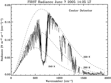
I’m wondering if he’s thinking of this graph, which is the Earth’s IR emission and shows that CO2 absorbs a substantial portion of its band?
‘…Earth’s IR emission and shows that CO2 absorbs a substantial portion of its band?’
That’s the ‘consensus’ interpretation of the so-called ‘notch’. If literally true, then there would be no sense in denying that ‘CO2 is the control knob’ of the Earth’s climate. Fortunately, there is no evidence for this from the paleo evidence, and as WE so aptly points out in his last two articles, continued attempts by alarmist scientists to show otherwise are complete garbage.
There’s no doubt that that is the CO2 absorption band!
H2O overlaps CO2 over much of the latter’s emission lines, especially when you account for the fact that clouds are mostly composed of water droplets and ice crystals, which as examples of condensed matter (unlike water vapor and CO2) can and do absorb and emit photons over the entire range of thermal radiation.
Further, per van Wijngaarden and Happer, CO2 doesn’t emit freely to space below 84km, so the emission you’re attributing to CO2 is actually confined to a very small peak (not really visible in the above graphic) at the bottom of the ‘notch’.
To put it simply, the thermal radiation from the Earth’s surface that is absorbed by GHGs is thermalized by collisions with non-GHGs within meters of the surface, meaning it is converted to sensible heat that is then convected aloft to where it can then excite GHGs at atmospheric levels conducive the spontaneous emission of photons to space.
The fact that most of this ‘work’ is done by H2O, rather than CO2, more adequately explains why, as I mentioned above, that there is no geological evidence that CO2 is the driver of the Earth’s climate, and also dovetails nicely with WE’s hypothesis that ’emergent phenomena’ acts as a negative feedback to maintain climate stability.
https://andymaypetrophysicist.com/wp-content/uploads/2025/01/Shula_Ott_Collaboration_Rev_5_Multipart_For_Wuwt_16jul2024.pdf
Exactly my thoughts about how the atmosphere works.
I suggest you reread van Wijngaarden and Happer, it doesn’t say what you think it does about CO2 emissions! The ‘notch’ as you call it is caused by absorption of IR by CO2 as I said.
I’ve read it several times before. I suggest you check out their Figure 6b from their ‘primer’ before casting any more aspersions. Also, if you read the work I cited above, they’ll explain to you why most folks misinterpret ‘the notch’.
https://arxiv.org/pdf/2303.00808
I repeat the ‘notch’ is caused by absorption of IR by CO2. I am well aware of what the Fig 6b means, it’s the result of selecting the strongest absorbing/emitting wavelength at 667.4 cm-1. This shows the effective emission height of that wavelength which is in the stratosphere, all the sidebands which contribute to the ‘notch’ have emission heights in the troposphere


‘I repeat the ‘notch’ is caused by absorption of IR by CO2’
Where? At the surface? Are you suggesting that Kirchoff’s Law applies to non-condensed matter, a la some sort of conservation of photons? Did you know that within meters of the Earth’s surface CO2 in an excited state is 50K times more likely to be deactivated by a collision with another molecule than by spontaneously emitting a photon?
Again, read the piece I cited earlier. If you have any issues, I’d be happy to discuss them.
“‘I repeat the ‘notch’ is caused by absorption of IR by CO2’
Where? “
In the atmosphere!
I’m well aware of the thermalization of CO2 in the atmosphere and have posted about it here many times.
I have read the piece you cited earlier and it’s seriously flawed. They make the assertion that “The process of thermalization results in the near extinction of most radiation in the absorption/emission of the GHG bands a very short distance from emission at the Earth’s surface.”
and then assert that: “The “notch” occurs because water vapor emissions begin to overlap with the CO2 absorption band, and the water emission is being absorbed by CO2. What the emission curve does not reveal is that the CO2 is then thermalized via collisions and that sensible heat energy drives additional thermally excited emission by water vapor.”
So the CO2 is thermalized but the H2O isn’t, contrary to their earlier statement!
The climate sensitivity of CO2, which has been derived in many publications for the current state of the Earth, is a function of CO2 concentration. At higher CO2 concentrations, it approaches zero. Furthermore, studies show that CO2 climate sensitivity has changed over the course of Earth’s history because other underlying conditions (continental drift, solar irradiance, etc.) have changed over millions of years. In my opinion, specifying a single mean value for the ECS for a period of 500 million years makes no sense.