Guest Post by Willis Eschenbach (@weschenbach on eX-Twitter)
Our estimable Charles the Moderator, who gets my eternal thanks for keeping the hits happening here on WUWT, asked me to take a look at a new paper yclept Multivariate Analysis Rejects the Theory of Human-caused Atmospheric Carbon Dioxide Increase:The Sea Surface Temperature Rules by Dai Ato, an independent researcher in Japan. Seems it’s been getting some play. I’ll refer to this paper as Ato2024.
I wasn’t far in before alarms went off. The study conducted a multivariate analysis using publicly available data to examine the impact of sea surface temperature (SST) and human emissions on atmospheric CO₂ levels.
It concluded that SST was the independent determinant of the annual increase in atmospheric CO₂ concentration. Human emissions were found to be irrelevant in the regression models.
And most revealingly, it says:
Furthermore, the atmospheric CO₂ concentration predicted, using the regression equation obtained for the SST derived from UK-HADLEY centre after 1960, showed an extremely high correlation with the actual CO₂ concentration (Pearson correlation coefficient r = 0.9995, P < 3e-92).
BZZZZT!! Whenever I get an r-value that high, I know for a fact that I’m doing something very wrong … I’ll get back to that.
First, let me start with one of the three variables in their analysis, which are SST, CO2, and emissions. Here are three reconstructions of SST since 1854 by three different groups.

Figure 1. Global monthly average sea surface temperatures (SSTs). Yellow area at the right is the portion of the record analyzed by Ato.
While there are some differences, overall the pattern is clear. There was SST warming from ~ 1850 to about 1870, cooling to ~ 1910, warming to ~ 1940, cooling to ~ 1965, and warming since then.
Looking at that, I can see why Ato doesn’t want to use the full record—it doesn’t support his claim that SSTs are the independent determinant of atmospheric CO2 levels. The CO2 data (Figs. 2 and 3 below) looks nothing like that.
So how does he justify the cutoff? Well, the Mauna Loa CO2 measurement data starts about 1960. However, it can be extended back beyond that using the ice core CO2 records. Here’s what that looks like.

Figure 2. Mauna Loa and ice core measurements of the background atmospheric CO2 levels, 1000-2010AD. Data: Ice Cores Mauna Loa
Ato2024 says that the ice core records are not accurate. However, this is belied by the close agreement of the ice core records with each other and with the Mauna Loa measurements as shown above.
Below is a closer view of the recent end of the data since 1850, corresponding to the time frame of the sea surface temperatures (SSTs) in Figure 1.

Figure 3. As in Figure 2, but post-1850 data only
As a result of the good agreement of the ice cores both with each other and with the Mauna Loa data, I see no problem in taking that as a good reconstruction of the post-1850 CO2 levels.
The problem, of course, is that the pre-1960 ocean temperatures do not look anything like the pre-1960 CO2 levels … and this disagreement totally falsifies Ato2024. So he is obliged to ignore it.
Next, how did he get such a great correlation, 0.9995, between SST and CO2 in the post-1960 data? In part the answer lies in what he looked at. Here’s the Mauna Loa post-1960 CO2 record he used. Note that he didn’t use the monthly data, just the annual data. Makes it easier to get a higher Pearson correlation coefficient “r”.

Figure 4. Mauna Loa Observatory CO2 observations, along with the linear trend line.
The recent increase in CO2 is a very slowly accelerating curve which is nearly a straight line. This leads to many false correlations because such a curve is easy to replicate as we’ll see below. This is a recurring problem in climate science.
But that’s just the first problem. The main problem is the procedure that he used. Here’s the description from the paper.

Note that the symbol delta (∆) in the equations means “change in”. So ∆CO2 is the change in CO2 from one year to the next.
Translated, that says:
- Calculate the best-fit linear estimation of the annual changes in CO2 (∆CO2), based on the Hadley HadSST sea surface temperature.
- The predicted atmospheric CO2 is then the starting atmospheric CO2 plus the cumulative sum of the estimated annual changes in CO2.
Here’s a graph of the first part of that calculation, fitting the SST to the annual change in CO2.

Figure 5. Post 1960 annual change in atmospheric CO2 (∆CO2), along with the linear trend line of ∆CO2, and the best estimation of ∆CO2 based on the Hadley HadSST4.0.1.
Now, there’s an oddity about graphing delta CO2, or ∆ anything for that matter. It involves a couple of curious changes. I’ll use graphing ∆CO2 as in Fig. 5 as my example.
First, any overall linear trend in the CO2 data is converted into an overall offset from zero (a non-zero average) in the ∆CO2 graph.
Second, any overall acceleration in the CO2 data is converted into an overall linear trend in the ∆CO2 graph.
So from looking at Figure 5, we can see that the ∆CO2 data has both a positive trend and an acceleration. We can see both of those in Figure 3 above.
And now that we’ve fitted the SST to the ∆CO2 data so we can estimate the ∆CO2, we simply sum those changes cumulatively to estimate the underlying CO2 data. Here’s that result.

Figure 6. Mauna Loa CO2 data, and Ato2024 estimation of the Mauna Loa CO2 data
At this point, I’ve replicated his results.
Now, remember that I said that a correlation coefficient of 0.999+ means there’s some fatal flaw in the logic. So … what’s not to like?
In his note asking me to take a look at this paper, Charles The Moderator included an interesting AI analysis of the paper, viz (emphasis mine):
Based on my analysis of the paper, the key issue of circular reasoning appears to be in the methodology used to predict atmospheric CO2 concentrations from sea surface temperature (SST) data. Specifically:
• The author uses multiple linear regression to derive an equation relating annual CO2 increase to SST for the period 1960-2022.
• This equation is then used to “predict” CO2 concentrations for the same 1960-2022 time period.
The predicted and measured CO2 concentrations are found to have an extremely high correlation (r = 0.9995).
The circular reasoning occurs because the same data is used both to derive the equation and to test its predictive power. The key equations involved are:
The regression equation (from Step 7 in the paper):
Annual CO2 increase = 2.006 × HAD-SST + 1.143 (after 1959)
The prediction equation:
[CO2]n = Σ[ΔCO2]i + Cst
Where [CO2]n is the predicted CO2 concentration, [ΔCO2]i is the annual increase calculated from the regression equation, and Cst is the actual CO2 concentration in the starting year.
By using this method, the author is essentially fitting the equation to the data and then using that same fitted equation to “predict” the data it was derived from. This guarantees an extremely high correlation that does not actually demonstrate any predictive power or causal relationship.
A proper analysis would use separate training and testing datasets, or employ techniques like cross-validation, to avoid this circularity.
The extremely high correlation reported is almost certainly an artifact of this flawed methodology rather than evidence of a genuine relationship between SST and atmospheric CO2 levels.
And the AI is right. Well, partly right. They’re right to say that the problem is not that Ato2024 fitted SST to CO2. The problem is that Ato2024 didn’t withhold half the data to verify the results. It’s easy to predict something when you already know the outcome …
HOWEVER, and it’s a big however … while that problem alone is enough to totally falsify the conclusions, there’s another really big problem. To illustrate that, I’ve used the Ato2024 method. But instead of using sea surface temperature as the input to be fitted to the ∆CO2 data as Ato2024 does, I’ve fitted a straight line to the ∆CO2 data. It’s the blue line in Figure 5 above.
And using the Ato2024 method, I’ve converted that straight line to the equivalent CO2 data shown in red in Figure 7 below.

Figure 7. As in Figure 6, plus a red line showing the result of using a simple straight line in place of the sea surface temperature (SST) used the Ato2024.
Interesting. Using the Ato2024 method of fitting a variable to ∆CO2, a straight line as input does just as as well as using the SST as input.
But that doesn’t really show the full scope of the problem. To do that, I first divided the SST, the straight line, and ∆CO2 data in two halves. I used the first half for fitting either the SST or the straight line to the first half of the ∆CO2. Then I used those results to estimate the change in CO2. Figure 8 shows that result.

Figure 8. As in Figure 7, but using only the first half of the data to fit the model, and then using the full data to see how well it performs.
This graph reveals two separate problems. First, although the fit is considerably poorer than in Figure 6, the Pearson correlation coefficient “r” is basically unchanged … meaning that it is not an appropriate measure for this particular issue.
Next, the straight line continues to perform just as well as using the SST as the independent variable … no bueno. This indicates a profound problem with the underlying Ato method.
To show the problem, I’m gonna re-show Figure 5 from above.
To recap, first, any overall linear trend in the CO2 data is converted into an overall offset from zero (a non-zero average) in the ∆CO2 graph.
Second, any overall acceleration in the CO2 data is converted into an overall linear trend in the ∆CO2 graph.
And here’s the key. When you fit the SST data (or more importantly, any data) to the ∆CO2 data, you end up with a fitted signal that has the same non-zero average and the same trend as the ∆CO2 data.
Not only that, but the fit will be balanced, with the amount above and the amount below the trend line being equal.
And all of that guarantees that if you start out trying to predict a smooth curve, when you reconstruct the signal using the method of Ato2024, you’ll get an answer that is VERY close to the smooth curve regardless of what variable you use to reconstruct the signal.
And that is why using the straight line does just as well as using the SST, or any other variable, as the basis for the estimation of CO2.
I weep for the death of honest peer-review …
My best to everyone,
w.
Yeah, you’ve heard it before: When you comment please quote the exact words you’re discussing. It avoids endless misunderstandings.
Figure 2 makes it clear he was cherry picking.
Not completely.
Assuming I understand what the estimable Honorable Eschenbach has written – what we have here is math games.
Math games by people who don’t actually understand what their math games are really saying.
So while there is cherry picking, the real problem is bad math.
What it reminds me of is Micheal Mann’s MBH98 “hockey stick” paper, which combined cherry picking and an algorithm that could make “hockey sticks” out of red noise.
But it was duly peer reviewed!!! Oh…
Well spotted, Charles. Well analyzed, Willis.
I am impressed that AI spotted a basic Ato logic flaw.
There is an independent physical reasoning way to refute Ato’s conclusion within his time frame. Most ocean CO2 is deep—not near the surface. So most of it cannot be outgassed by a change in surface temperature in Ato’s timeframe. (Average ocean depth is 4000 meters, average surface mixed layer is 150 meters.) A single ocean bottom water overturning takes between 800-1000 years (estimates vary but are all in this near millennial time frame). In that time frame, Gore’s famous ‘Inconvenient Truth’ curve does indeed show ocean temperature leading CO2—the opposite of what Gore claimed.
“I weep for the death of honest peer-review …”
well that is the whole point of the supposed journal “Science of climate change”. It is a bottom feeder journal designed to take money from the gullible and vain by publishing their work. Sometimes you can judge a book by its cover.
Which is Willis’ point. Here there was no peer review, as you note. In the mainstream “prestige” scientific journals there is peer review, but less and less of it is honest. That makes it hard to distinguish the bottom-feeders from the apex journals sometimes.
The pay-to-publish journals are at least open in how they operate. Others that pretend to be pure, but play favorites through pal review, are hypocrites and should bear the most shame.
I am unimpressed by peer review even in the most prestigious journals Science and the Nature stable. In ebook Blowing Smoke I identified four cases of outright academic misconduct not caught by peer review. One was by comparing to background thesis (which peer review would not have caught), two by info in the accompanying SI, and one from estuary first principles. Peer review should have caught the last three—but didn’t. All in the most prestigious journals.
I had a similar experience with Nature some years ago. The conclusion of a paper about nitrate pollution turned upon an artifact.
I wrote up a short note, including a graphic showing the problem, sent it to Nature and was politely dismissed.
At least they were polite! 🙂
Dunno about that Izaak.
“The Compleat Angler” is a fabulous book.
You wrote it, remember.
Did you get it peer reviewed before publication?
Every journal that publishes a paper falsifying the consensus is a bottom feeder journal designed to take money from the gullible and vain in your estimation, Izaak.
So, whatever the true status of that journal, your opinion of it can be discounted as unreliable.
Article needs more about what the original author Ato intended to convey to his readers and what it would mean on the grander scale if he were right/wrong.
It’s in the title of Ato’s paper:
I think you can extrapolate on your own what that might mean.
Willis,
Thank you for helping Charles out with this article and I second your thanks for all the work he does here.
I also appreciate your style. You made me laugh when I read
And most revealingly, it says:
“Furthermore, the atmospheric CO₂ concentration predicted, using the regression equation obtained for the SST derived from UK-HADLEY centre after 1960, showed an extremely high correlation with the actual CO₂ concentration (Pearson correlation coefficient r = 0.9995, P < 3e-92).”
In my initial read I skimmed over the details over the r-value until I read your description:
BZZZZT!! Whenever I get an r-value that high, I know for a fact that I’m doing something very wrong … I’ll get back to that.
Before I went back to see the R value I thought well high could it be. High to me would be 0.9 or thereabout. Then I read that it was claimed to be 0.9995 and burst out laughing. As you said that high a number means something is wrong and anyone who doesn’t pick up on that is way off base.
Thanks for clearly explaining exactly why the analysis went off the rails.
Thank you to Willis and Charles for this good discussion of this paper.
Willis,
Congratulations on a very fine analysis, explaining clearly th many problems in the article.
“I weep for the death of honest peer-review …”
Yours may well be the first peer review. The article did not appear in any regular scientific journal. SCC is, well, they say it themselves:
“The objective of this journal was and is, to publish – different to many other journals – also peer re-viewed scientific contributions, which contradict the often very unilateral climate hypotheses of the IPCC and thus, to open the view to alternative interpretations of climate change. “
Chief editor is Monckton’s mate Hermann Harde.
The thing that first set me off was the insistence on using “UAH-SST”. Now of course UAH does not claim to measure SST. It measures temperatures in the lower troposphere.
What the paper has in common with many analyses claiming to show the CO2 in the air is not of human origin is that they work using differences. The real pattern of the data is that our cumulative emissions rise fairly steadily, and so does CO2. There is some correlation between annual-scale fluctuations of CO2 and SST. But what ATO and others do is an analysis in which the mean of differences is subtracted out. This is the whole effect of that steady rise together of cumulative emissions and CO2 in the air, just dropped from the analysis.
So Nick, is what you’re saying is that correlation = causation?
Say it isn’t so 🙁
It is Ato who wrote a paper based on multivariate correlation, not I.
“The thing that first set me off was the insistence on using “UAH-SST”. Now of course UAH does not claim to measure SST. It measures temperatures in the lower troposphere.”
What sets me off is people claiming they know what the sea surface temperatures were since the Little Ice Age ended.
Phil Jones says they were just guessing at the sea surface temperatures. That’s all we have is guesses, and those guesses come from Climate Alarmists like Phil Jones.
Using sea surface temperatures created out of thin air and the fevered imaginations of Climate Alarmists has misled the world into believing things that are not true, like today being the hottest time in human history.
The only real evidence we have, the written, historic temperature records show this is false. The written temperature record shows it was just as warm in the recent past as it is today, and this shows that CO2 has had no discernable effect on the Earth’s temperatures since there is more CO2 in the air today than in the past, yet it is no warmer today than it was in the past with less CO2 in the air..
A couple of questions for Willis:
It is extremely important that in all these arguments about models, they must be subjected to actual known physical and chemical processes, and not be merely correlations, some of which work better than others. Without known processes to describe what is taking place that justify the correlation, correlations without causation produce bullshit conclusions.
A model based on statistics is not science based on data.
That is my read of what you posted.
It’s not that statistics don’t matter. Almost everything produced by man is backed up with some kind of statistic, whether in business or science or engineering or sports, which all people use every day. How many times a day do you or most people refer to the term “average”, or “maximum” or “minimum” or rate of something? That’s statistics too.
It is that correlations that are not tethered to actual known phenomena are useless. This happens all the time in junk science, not just junk climate science, but other areas as well such as correlations between various chemicals and human health, or between various diets and human health and longevity. It’s like saying, “People who eat cat poop have lower intelligence than people who don’t eat cat poop, so eating cat poop must therefore lower your IQ.”
Very interesting. I don’t know the history of multiple regression but it is old and used to be in advanced statistics along with curvilinear, complicated as it was. It may have become a fad when computers could handle it. It sounded good for ecosystems but still requires too many hypotheses and their variables, models as they are now called. Peer review then didn’t have “impact factors” to consider and computers to organize their analyses.
Multiple regression has been around for ages. The most common variant is ‘ordinary least squares’ aka OLS. It is mathematically valid when the analysis conforms to the ‘BLUE’ theorem requirements (aka best linear unbiased estimate). Often it is necessary to do some x data transforms to get to BLUE. Is taught as part of basic statistics and econometrics.
’Multiple’ just means that rather than one independent variable (x) used to estimate y, there are more than 1 (x1, x2,…). Things get dicey when there are many xN, because the BLUE theorem gets harder to satisfy. on the other hand, leaving out an important X term also invalidates the result.
I was suspicious when I saw the very high r value, but I don’t think the relationship between temperature and CO2 growth should be dismissed because of this paper.
When there is a large or prolonged increase in temperature, there is an increase in CO2 growth. When there is a large or prolonged decrease in temperature, there is a decrease in CO2 growth.
Below is a graph of change in annual University of Alabama Huntsville (UAH) Globe temperature anomaly and change in CO2 growth over time from 1980 to 2023.
The hard part is explaining why this is happening. If atmospheric CO2 and oceanic CO2 were in equilibrium then a fall in temperature should result in a fall in the amount of CO2 in the atmosphere. However, what we observe is that a fall in temperature results in a fall in the rate of increase. This suggests that the system is equilibrating and that the equilibration rate is temperature dependent.
This allows us to make testable predictions. After the recent big spike in warming, caused in part, I suspect, by the Tongan eruption putting all that water in the stratosphere, I am expecting there to be a significant drop in the temperature once Dr. Lindzen’s “Iris effect” kicks in. When this happens I predict it will be accompanied by a corresponding drop in the rate of CO2 growth.
Here is the cross plot for change in UAH globe annual temperature anomaly versus change in CO2 growth for the period 1980 to 2023. The only manipulation of the data I have done was to calculate the annual average for each year. UAH doesn’t publish an annual value for the temperature anomaly.
Notice the r-squared is only 0.37 and not 0.99
It isn’t a great r-squared but given the nature of the data, it isn’t dreadful.
The relationship shows up in other temperature datasets. I have looked at NOAA’s NCEI, NASA’s GISStemp and HadCRUT5. I think it is interesting that the relationship is present in these datasets despite the adjustments that they have been made to the raw data.
A caution. Correlation is not causation. See my comment above concerning an independent physical ocean disproving Ato.
“Correlation is not causation.” Indeed. My favorite correlation is between protestant preachers and unwanted pregnancies per square mile in the state of New York.
Joking aside, there is a good theoretical reason why temperature and atmospheric CO2 ought to be related. That is the change in CO2 solubility with temperature of which I know you are aware. The fact that the CO2 in the deep ocean can’t rapidly take part in the process does not mean surface water does not participate in the equilibrium relationship.
A change in the ocean heat content ought to change the proportion of CO2 in the atmosphere.
I am not defending Ato’s paper. Willis’ explanation makes sense and the .99 correlation was a definite red flag.
Note that an r-squared of 0.371 is a correlation (r) of 0.61 or 61%.
The interesting thing for me is that it is a change in the rate of change in CO2. Assuming the relationship is real, and it seems to be, it means that a drop in temperature correlates with a drop in the rate of increase in CO2. However, the drop in the rate of increase does not take the rate below zero. So that means we have a drop in temperature correlating with an increase in CO2. Which is not what the global warming hypothesis predicts. This means that CO2 is not the independent variable.
Proponents of the idea that CO2 is increasing because of anthropogenic emissions usually use two arguments. The mass balance argument and the isotope ratio argument. Neither of these take into account the equilibrium relationship, which I am arguing, mostly controls atmospheric CO2 content and change.
I agree with respect to surface waters. Beer is proof enough of Henry’s Law. I am arguing an irrefutable carbon relative isotope mass balance on oceanic relevant time scales.
John, There is an interesting web site that provides numerous correlations, all spurious at https://tylervigen.com/spurious-correlations
Their most recent at the first page is “The Distance Between Saturn and the Moon Correlates with Bachelor’s Degrees Awarded in Physical Sciences” The R^2 is 0.987.
However, while the average residence time of deep, carbonated water is of the order of 1,000 years, that can be short-circuited by up-welling along the western coasts of the continents. The South American up-welling is strongest during La Nina years, suggesting that the up-welling doesn’t play a strong role in increasing atmospheric CO2. It is probably the warming effect on bacteria feeding on dead photosynthetic organisms, and the increase in boreal tree Winter respiration during El Nino events that are responsible for the observed increase in the seasonal ramp-up phase of atmospheric CO2.
I’m leery of the mass-balance argument because I suspect that there is a subconscious bias to be sure that everything is balanced in the Carbon Cycle before the anthropogenic emissions are taken account of. I believe that the ocean CO2 and boreal Winter respiration fluxes are poorly known, but still used with an assumed high accuracy.
Similarly, I don’t think that the isotope arguments are robust because I’m of the opinion that isotopic fractionation is not well characterized for things like out-gassing and dissolving of CO2, and utilization of carbon isotopes for calcifiers with different optimal pH requirements.
John, the equilibrium between SST and CO2 in the atmosphere for the current average SST is around 295 ppmv, some 9 ppmv up since the LIA. Maximum change due to temperature: some 16 ppmv/°C over 800,000 years ice ages/interglacials. That is all. See my extensive comments next page…
We are at some 125 ppmv over that equilibrium, thus the net CO2 flux is from the atmosphere into the oceans (and the biosphere). The year by year fluctuations since 1958 are not more than about +/- 1,5 ppmv around the 100+ trend for the extremes (Pinatubo, El Niño), while humans emitted over 200 ppmv in the same time frame. If the natural variability also was the same in the long past, that was not even visible in the best resolution ice cores (Law Dome, less than a decade).
About the isotopic change: not more than +/- 0.4 per mil over the past 800,000 years, -2 per mil since 1850, both in the atmosphere (ice-firn-air) as in the ocean surface:

Hi Ferdinand.
“Maximum change due to temperature: some 16 ppmv/°C over 800,000 years ice ages/interglacials.”
My problem with this is that I don’t think it is reasonable to assume that the CO2 content of an ice core air bubble tested today is necessarily an accurate measure of the CO2 content of the air when the snowflakes fell. This is because CO2 can permeate through the solid ice if given enough time. When a snowflake forms there is no CO2 dissolved within the frozen water. Over time the CO2 in the air bubbles trapped in the ice will diffuse into the ice, reducing the concentration of CO2 in the air bubbles. Because of this, I don’t think it is reasonable to rely on the 16ppmv/°C value. BTW, that is about the number I get from the ice core data, but I don’t trust the absolute values for those data.
John,
Diffusion through the ice matrix is impossible for CO2 and other gases, only possible via water-like veins between the ice crystals and down to -32°C, below that there is certainly zero water left between the crystal borders, except around dust inclusions, which are rare in Antarctica.
Theoretical migration was measured in the relative “warm” ice core of Siple Dome (-23°C) near a melt/refreezing layer and resulted in a broadening of 10% in resolution (20 to 22 years) at middle depth up to a doubling in resolution (~40 years) at full depth at 90,000 years BP. Not a big deal.
For the long-term ice cores like Vostok (420,000 years) and Dome C (800,000 years) below -40°C, no measurable migration exists.
If there was even the slightest migration, the ratio between CO2 and T over time would fade, for which is not the slightest indication after 800,000 years:

If there was migration, but compensated by increasing CO2 levels during interglacials farther back in the past, as the late Dr. Salby once postulated, then the CO2 levels during glacials should have been negative before migration from the second glacial period on…
Moreover, the newer sublimation technique, used for isotopic detection, shows that as much air is included in every part of ice (with bubbles or without – only clathrates) and no CO2 or other gas can hide anywhere as 99.9% of all gases are recovered…
Forgot to give the reference to the “migration” paper:
https://catalogue.nla.gov.au/catalog/3773250
john, what browser are you using? Neither Firefox (Mac) nor Safari include a button for graphic upload.
Hi Pat. I’m using Mozilla Firefox. I am uploading jpg, not png. Not sure why you can’ upload.
There is a little icon on the bottom right that looks like a couple of mountains. Just above the Post Comment button.
I’m using Firefox and it’s not there for me.
I am on android/windows. If you are on Mac, perhaps that is the reason. Do you have access to a not Apple machine?
I use Firefox (Windows) and it is there for me. It appears after you click on “reply”.
Should be right here.
I remember it from the past. It’s not present for me on Firefox or Safari.
Pat, I’m using Firefox and it shows up at the right bottom as I’m typing this.
It’s not there for me, Clyde.
It is particularly noticeable during El Nino years when the slope and peak of the seasonal ramp-up phase are larger than other years. However, when the El Nino ends, the ramp-up phase curve returns to the former shape.
Willis is correct that Ato is using circular reasoning to show that the change in CO2 concentrations is ONLY a function of sea surface temperatures. While this tends to shift the cause of increasing CO2 concentrations from human CO2 emissions to a natural cause such as changes in sea surface temperature, the change in human CO2 emissions can’t be discounted entirely.
I have previously performed an analysis of the dependence of CO2 concentrations (at Mauna Loa) on human CO2 emissions from 1959 to 2023, without accounting for changes in sea-surface temperatures. This resulted in the following regression:
8.006 dC/dt = E(t) + 39.92 – 0.140 C (Eq. 1)
where C = atmospheric CO2 concentration in ppm
E(t) = human CO2 emission rate for year t, Gt/yr
The factor 8.006 Gt/ppm represents the mass of CO2 required to raise the concentration of the entire atmosphere by 1 ppm. The last term in the above equation represents a first-order rate of removal of CO2 by natural processes, including photosynthesis. The above regression had a correlation coefficient of r^2 = 0.8311 (r = 0.9116).
The above equation shows that if human CO2 emissions remain constant, the CO2 concentration will not increase indefinitely, but reach equilibrium when dC/dt = 0 at a concentration of
Ceq = (39.92 + E) / 0.140 (Eq. 2)
Global human CO2 emissions were estimated at 37.2 Gt/yr in 2022. If that rate was held constant, the CO2 concentration would level out at 551 ppm, sometime after AD 2200.
The 39.92 Gt/yr represents total natural emissions of CO2 to the atmosphere, which can include outgassing from the oceans, but also CO2 emitted from animal and human respiration, fires started by lightning, and other natural sources.
In order to include the sea-surface temperatures in the above model, Equation 1 could be modified as:
8.006 dC/dt = N + a Ts(t) + E(t) – b C (Eq. 3)
where
N = natural CO2 emissions independent of sea surface temperatures(Gt/yr)
Ts(t) = sea surface temperature, or a global-average anomaly
a (Gt/yr-K) and b (Gt/yr-ppm) are constants of a multivariate regression.
The relative values of N, a, and b would determine how the following factors control CO2 concentrations in the atmosphere: sea surface temperatures, natural emissions, human emissions, or photosynthesis.
This is not an expression of any opinion on the matter, but a suggestion for further study.
Hi Willis
So how is that with the paper from K? Could you have a look at that as well, please?
https://wattsupwiththat.com/2024/08/30/new-study-co2s-atmospheric-residence-time-4-yearsnatural-sources-drive-co2-concentration-changes/
He sees the human contribution to delta CO2 in the atmosphere as only 4%, the rest is coming from delta SST.
Simple analytical chemistry leads me to believe that A and K and at least 3 others that I know of are right and that all human made CO2 that is not being immediately used by the bio-sphere simply disappear as carbonates in the deep ocean. Delta SST is the cause of delta CO2 in the atmosphere whichever way I look at it.
HP, not Willis but a sharp response. K (and earlier Salby) confound residence time with efold time. Plus, K’s carbon isotope ratio ‘data’ does not agree with that from any other institution, including NOAA from Amundsen Scott and Scripps from more than the stations used by K. The ‘mostly natural’ argument is disproven now several ways. This bogus paper is but one.
The winner argument is NOT that the observed rise is not anthropogenic, since it probably is. The winner is that it doesn’t matter much—models saying otherwise provably wrong, Earth greening, no previously predicted bad stuff has happened…
Thanks, Rud. I was about to make that same point about his post conflating residence time and e-folding time, but fortunately I read your comment first.
w.
It seems that the K’s paper on the CO2 isotopic C13 fraction needs a careful reading :
https://www.mdpi.com/2413-4155/6/1/17
In this paper, K. does not refute the atmospheric CO2 C13 fraction as measured by 4 measurements stations, instaed, he actually uses them for his study.
Measurement stations used in K.’s paper :
Barrow, Alaska PTB 71.3° N, 156.6° W
La Jolla Pier, California LJO 32.9° N, 117.3° W
Mauna Loa Observatory, Hawaii MLO 19.5° N, 155.6° W
South Pole SPO 90.0° S
So, the claim that his findings are not in agreement with the atmospheric CO2 C13 measured fraction is wrong (which does not mean that his paper is right).
The point of his study is to evaluate the net CO2 input CO2 C13 fraction in the atmosphere (not the global atmospheric CO2 C13 fraction), and to achieve this, K. actually uses the 4 official measurements of the atmospheric CO2 C13 fraction.
He finds that the net CO2 INPUT C13 fraction has increased during the last 60 years and is currently -13,3 per thousands.
Again : with respect to the CO2 C13 fraction, these results on the net CO2 input (net CO2 emission flux) right or wrong as they might be, are not in contradiction with the 4 official measurements carried on the atmosphere CO2 stock.
Moreover, the -13.3 per thousands obtained current value of the net input fraction is not in contradiction with the observed decrease trend of the atmospheric stock fraction (currently about -8.4 per thousands), since it is smaller.
Hope this will clarify K.’s paper which, again, seems to deserve a careful reading.
Petit-Barde,
There are only two sources of low-13C in this world: fossil organics CO2 at average -25 per mil δ13C today and recent organics at average -24 per mil δ13C, if they are decaying by molds or bacteria or eaten by animals and humans. Or +24 per mil δ13C if photosynthesis takes preferentially 12CO2 out of the atmosphere.
All inorganic CO2 (oceans, carbonate rocks, volcanic vents,…) is around zero per mil δ13C.
Thus the enormous decline of δ13C since 1850 is either from fossil fuels or from vegetation or a mix of both.
The oxygen balance definitely shows that the biosphere is a net absorber of CO2 (the earth is greening), thus increasing the δ13C level of the atmosphere, thus fossil emissions are the sole cause of the δ13C decline…
Koutsoyiannis used the “apparent” fixed supply of -13.3 per mil to assume that the increasing drop in δ13C was not caused by fossil emissions, but didn’t take into account that the fossil “fingerprint” is redistributed over more reservoirs and especially didn’t take into account the long return of “old” CO2 from the deep oceans, from long before human emissions (or the atomic bomb spike)…
Here the δ13C level in the atmosphere for different deep ocean returns:
Ferdinand,
K. makes no assumption on d13, he uses the stock atmosphere d13 as officially measured and the CO2 mass balance equation (see paragrah 3. Theoretical framework).
K.paper’s result is that the net CO2 input d13 is increasing.
The only point is : is K. correct ?
The “returning CO2 from oceans after a long period from previous anthropogenic absorption” assumption (propagated by the IPCC to justify a response/adustment time of decades if not centuries) is pure fantasy :
There is no causal link between 2 processes (absorption, and a long time after, emission) since during this “long time”, there are too many and massive (wrt the 2 processes above) reactions in the oceans that affect its own CO2 concentration and also the CO2 solubility (vents, volcanoes, fluxes between layers, balances with other components as Ca, absorption by marine photosynthetic organisms (which represent almost all the atmospheric O2 source), sea temperature variation, marine biomass respiration, etc.).
With respect to oxygen :
Almost all of the atmospheric oxygen is emitted not by terrestrial vegetation but by marine photosynthetic organisms (cyanobacteria and plancton) using HCO3- which is regulated in water by many reactions (see above).
Vegetation ecosystems are not net CO2 sinks. As an example, rainforest ecosystems emit more CO2 than the vegetation absorbs by phtosynthesis because there is massive biomass respiration under the canopy.
For the same raison, rainforests are not the planet O2 main source (actually they are not even a O2 significant source : most of the emitted O2 is indeed absorbed during the biomass respiration).
Petit-Barde,
Not Ferdinand here, but I am familiar with the Keeling plots that Koutsoyiannis uses. I am unsure why you say “K.paper’s result is that the net CO2 input d13 is increasing.” Sorry if I am misunderstanding you, but his use of the Keeling plot (his figure 10) demonstrates that the average net δ13C of the incremental atmospheric CO2 has been constant at around -13%, not increasing. This is true for the entire period of direct measurements (since the late 70s) and, if you accept the Law Dome data, going back to the end of the Little Ice Age. It is actually trivial to confirm this as it can be determined simply from the CO2 concentration and its δ13C value. If you accept mass balance principles, which must apply to 12C and 13C (both stable isotopes), the result is unambiguous.
You can even use a quick calculation between any two sets of pairs of atmospheric CO2 concentration and the δ13C value. There is a very small approximation in this calculation, but it is widely used in the literature.
Take, for example:
280ppm and -6.4% (pre-industrial mean, circa 1750, Böhm et al (2002))
336ppm and -7.49% (Scripps CO2 Program, December 1979)
409ppm and -8.49% (Scripps CO2 Program, December 2019)
Between 1750 and 1979:
Average δ13C=((336*-7.49)-(280*-6.4))/(336-280)=-12.9%
Between 1979 and 2019:
Average δ13C=((409*-8.49)-(336*-7.49))/(409-336)=-13.1%
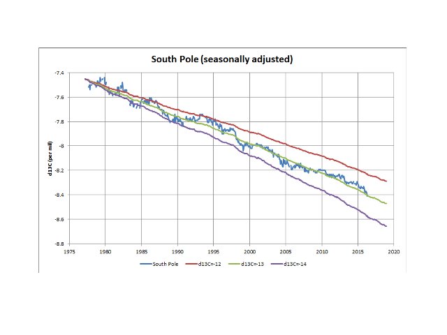
These values reflect the long term average, but do not capture variations in trend. That’s where Keeling plots assist in showing such variations that may exist. I make no comment on the interpretation of the data, only on the validity of the data in determining the average net effect on atmospheric δ13C value. Finally, here is a plot of South Pole δ13C measurements which highlights the unambiguous evidence for the decline in atmospheric δ13C reflecting an average net value of -13‰ for the incremental CO2 (the three lines reflect atmospheric δ13C values based on actual CO2 measurements, but with an assumed constant δ13C content of -12‰, -13‰ and -14‰, overlain on the actual δ13C observations):
The relevant material balance equations and the basis for the Keeling plots can be found here: Kőhler et al (2006) (pdf).
Sorry (again) for my error in copying and pasting % instead of ‰ for most of the δ13C values. Perhaps I should go back to using “per mil”!
Petit-Barde,
Koutsoyiannis used the δ13C change as “proof” that human CO2 is not the cause of the extreme δ13C decline since 1850, which simply is absurd.
In ice cores over extreme differences in temperature and CO2 levels, the δ13C level didn’t change with more that 0.4 per mil in 800,000 years.
isotope measurements are always done with the sublimation technique, which recover all gases (even out of clathrates) for 99.7% to avoid fractionation. Here the result:
Since 1850 there is a drop of 2 per mil δ13C in the atmosphere and in the ocean surface. Equivalent to the destruction of about 1/3 of all vegetation on earth, if that was the cause, while vegetation in reality, both on land and in the oceans, is INcreasing, not DEcreasing…
The oxygen balance doesn’t make a differentiation between where the sources and sinks are, it is just bookkeeping. Fossil emissions are rather accurately known (tanks to sales – taxes) and how much oxygen they use can be calculated per fuel type. The measurements in the atmosphere of the O2 decline, minus fossil use of O2 gives how much the biosphere did release or absorb of O2. That is what was measured in the period 1993-2002 by Bender et al:
With as result a net uptake by the whole biosphere (land + oceans) of 1.0 +/- 0,6 PgC/year.
There was a more recent update, but didn’t find a reference to that investigation…
The IPCC doesn’t include a return from the deep oceans at all, because in the Bern model the ocean surface completely isolates the deep oceans from the atmosphere and limits its uptake, as the ocean surface is saturated already at only ~10% of the changes in the atmosphere. That is the Revelle/buffer factor of the ocean surface waters.
The graph of the different returns refutes the Bern model: if there was no return (0 GtC/year), then the drop in δ13C would be some three times sharper in the atmosphere than observed, as all fossil emissions would remain in the atmosphere, besides some small redistribution in the fast cycles with ocean surface and biosphere…
Just because someone wrote a bad paper that is easily disproved, it does not prove that humans are responsible for the CO2 growth. It only proves that the paper cannot be used to support the thesis that it is “mostly natural.” If only it were so simple to dismiss the likes of Hansen and Mann by writing bad papers that ‘supported’ them.
Clyde, humans emit some 5 ppmv/year directly into the atmosphere. 100% of the emissions start in the atmosphere, thus add to the total CO2 amount in the atmosphere and nowhere else.
Only half of that increase is measured in the atmosphere.
Thus the main question is not what caused the increase, the question is where did half the fossil emissions go?
And that is not about the individual fossil CO2 molecules, that is about the total mass of CO2 added. Even if all individual fossil CO2 molecules were cached by the next available trees, that was at the cost of “natural” CO2 molecules which then remain in the atmosphere, the total amount of CO2 remaining in the atmosphere getting exactly the same…
Willis, a nit-picky edit for your text prior to figure 7: you refer to the blue line in figure 3, but I believe you meant figure 5.
Thanks, Wayne, fixed. I hate typos.
w.
Before I Comment on your analysis, I would like for you to comment on mine at retiredresearcher.wordpress.com.
Good stuff, Fred. I like it. Like I said. I can come to the same conclusions that you made, just by looking at the chemical equations that are relevant, and the moon shaking the erlenmeyer up everyday.
What is the exact address for your paper? I’m 80 years old and not too swift with these fancy computers.
Which spreadsheet are you using? You mention its limited data capacity. I think gnumeric has increased its sheet size to at least match excel.
Otherwise R.
I’m still using 123.
The top a-b graphic showing mid troposphere well-mixed CO2 and sea surface temperature – what is its origin?
There was also criticism of this Ato paper on Judith Curry’s blog Climate Etc.
https://judithcurry.com/2024/08/25/extension-of-the-linear-carbon-sink-model-temperature-matters/#comment-1009875
Scientist Dr Joachim Dengler wrote the main article article on “Extension of the linear carbon sink model – temperature matters”. A reader asked his opinion of the related Ato paper and there is discussion in comments.I also commented, noting that the Mauna Loa record is culled in ways that could affect the sense of both Dengler’s and Ato’s work and that early atmospheric CO2 concentrations should not be assumed to be 280 ppm or so, given the numerous pre-industrial chemical analyses above 300 ppm reported in the large compilations by Beck
https://journals.sagepub.com/doi/10.1260/095830507780682147
….
Too many corners are cut in too many climate papers. I can only join the lament for the failure of proper peer review.
Geoff S
Did you get full access to Beck’s paper? If so, how did you do it?
Using Google, you should obtain the essay, “Climate Change Reexamined” by
Joel M. Kauffman. The essay is 26 pages and can be download for free.
Shown in Fig. 7 is the IR absorption spectrum of a sample of Philadelphia city air from 400 to 4,400 wavenumbers. Integration of the spectrum by planimeter determined that H2O absorbed 92% of the IR light and CO2 only 8%. This integration must have been very tedious due the fine structure of the coupled rotational-vibrational structure of the H2O peaks. Since the wavenumber scale is linear in energy H20 absorbs much more IR energy than CO2.
This spectrum shows that H2O is the major greenhouse gas and CO2 is a trace greenhouse gas. This spectrum can be used (1) to shut down all this nonsense that CO2 is “menacing molecule” that is causing “global warming and climate change” and (2) to expose the claim by the IPCC that CO2 is the cause of “global warning”
is a lie.
Do you know how download Fig. 7 and display it here at WUWT with my above
explanation? The challenge is to inform all the people of the lies and fraud being
perpetrated by IPCC.
You should also check out Fig. 10. This plot of the CO2 data from Beck’s earlier paper.
Finally, I live in BC, Canada. The carbon tax is $80 per tonne of CO2 equivalent.
This tax has caused a significant increase in the cost of food and fuel. PM Justin Trudeau has decided to increase the carbon tax to $170 per tonne of CO2 equivalent by 2030. This is crazy. Canada has very cold winters.
Harold,

While criticising those who cut corners, when writing my comment here I did a quick search for a link to Beck by Google. Search term on my i-phone was rough (before sunrise, in bed, just out of hospital the day before). I used
“Bech early co2 analysis”.
It gave a link that I used without further examination because I have the several Beck papers filed on my PC. Sloppy on my part, sorry.
However, a Beck reference that I have studied a lot is
https://www.researchgate.net/scientific-contributions/Ernst-Georg-Beck-2015573085
Beck wrote “More than 90,000 accurate chemical analyses of CO 2 in air since 1812 are summarised. The historic chemical data reveal that changes in CO 2 track changes in temperature, and therefore climate in contrast to the simple, monotonically increasing CO 2 trend depicted in the post-1990 literature on climate-change.”
…..
Here is figure 7 from Kauffman
This was from a Google scholar search for kauffman, a screen cap, an image in Corel PhotoPaint and a URL in my private web hosting site.
……
After all that, yes, a most interesting Figure 7.
We did atomic spectrometry in the 60s when i was at Uni and not much on molecular. It was still developing, so I am undereducated. However, the simple message in Figure & is as you report. Its spectrometric effect in the air is tiny compared to water vapour, which many people know but few people write about.
For 20 years I have been critical of “doubling” of CO2 methodology, wondering why the doubling should not start from a base of 1 molecule of CO2 becomes 2 molecules. The atmosphere has about 4.1*1040 molecules of carbon dioxide which is a lot of doublings to present level.
….
If your point is that there is too little CO2 to do much, seems I agree. A commenter named Dr Strangelove some time ago maintained that
Energy of 15 um IR photon from Planck’s law:
E = h c/w = 1.32 e-20 J
where E is energy, h is Planck’s constant, c is speed of light, w is wavelength
Kinetic energy of CO2 molecule:
E = KE = 1/2 m v^2
m = M/N
where KE is kinetic energy, m is mass of molecule, v is velocity of molecule, M is molar mass of CO2 = 44 g/mol, N is Avogadro’s number
Solving for v^2
v^2 = 2 E/m = 3.6 e5
Mean kinetic temperature of gas from kinetic molecular theory:
T = v^2 M /(3 R)
where T is mean kinetic temperature, R is ideal gas constant
T = 635 K
You see there’s enough energy in IR to increase gas temperature. CO2 is only a trace gas in the air that’s why we don’t get this high temperature.
…….
Willis, I do not want to sidetrack your excellent article which says a lot about confused methods, so these comments of mine can be taken as more confusion.
Geoff S
Transcription error
Should be 4.1*10^40 molecules
Geoff S
Wow! Your graphic of the IR spectrum of the warm, humid Philly air is amazing and is twice as big as the original. Putting title of Kauffman’s essay at the top is nice attention to detail, the mark of a professional.
At the bottom of figure caption there is a reference to “The Journal of Chemical Education”. The title of the short paper is “Water in the Atmosphere” and the reference is: Journal of Chemical Education,
Vol. 81 No. 8 August 2004, pp 1229-1230. Unfortunately the journal
is now behind a paywall.
When I look at the spectrum, I now have no doubt that H2O is by far the major greenhouse gas and that CO2 is a trace greenhouse gas and can only cause a very small amount of warming. In discussions
of the greenhouse effect (GHE), I can use the spectrum to inform participants that the IPCC is not telling the the truth about CO2’s role
in the GHE.
I think it would be a good idea that you post the spectrum and a
short explanation of the role H2O in GHE at the beginning the next
“Open Thread”. However, I have my doubts that most people won’t pay attention. Anyway, think this over.
Awhile back, I asked Willis to post the spectrum here at WUWT be never replied.
The challenge is to form the people and politicians about the GHE and what the UN and the UNFCCC are really up to.
Geoff, I had very intensive discussions with the late Ernst Beck until his untimely death in 2010.
The problem with his reanalyses is not the so much the accuracy of the measurements of that time (+/- 3% or +/- 9 ppmv), but where was measured: in the middle of towns, forests, under, within an just above growing plants,… Completely unsuitable as “background” CO2 measurements,
Ice cores CO2, stomata data, coralline sponges data all contradict the 80 ppmv “peak” of his compilation…
See my web page of the past discussion:
http://www.ferdinand-engelbeen.be/klimaat/beck_data.html
Last year, there was a post-mortem publication of his latest work at SCC:
https://scienceofclimatechange.org/wp-content/uploads/Beck-2010-Reconstruction-of-Atmospheric-CO2.pdf
And a critique on that work by me:
https://scienceofclimatechange.org/wp-content/uploads/Engelbeen-2023-Beck-Discussion.pdf
And an explanation of the “peak” by Hermann Harde:
https://scienceofclimatechange.org/wp-content/uploads/Harde-2023-Historical-Data-Beck.pdf
and a few more recent, that I hadn’t seen before on the website of SCC…
Ferdinand,
Thank you for your comments, most of which I was aware from previous reading.
The basis for my concern is more logical than chemistry or physics. One way to put it, if you are going to reject some measured CO2 concentrations, you have to provide reasons. It is not enough to say that the sample location was unsuitable – the CO2 at every location is potentially able to do radiative physics that add to the total picture, unless you show it cannot. There has also been too little attention to paths of CO2 between emission and sink and we know from examples like corn fields that there are CO2 micro circuits where CO2 never gets near ML or Cape Grim. I do not know the size of these aggregated micro circuits but I do not discount that the discussed 50% of anthro that vanishes could be explained by mass balance errors from assuming well mixed. This might sound way out, but it has not been researched enough to allow it to be ignored.
Then, on Henry’s Law, my concerns are that the conditions in the lab for calculations of factors are vastly different to the open oceans with winds, waves, stratification of temperature, pH and salinity, high ionic strength, buffering, diurnal energy changes, seasons, active biological processes involving CO2 – oceans can be sources or sinks at different times and places. It is a complex dynamic system that requires great care for the valid use of Henry’s Law.
Re the Koutsoyiannis work on direction of causation, temperature driving concentration or reverse, there are papers by him with maths far beyond my capability so I cannot contribute.
Geoff S
Geoff,
The main 1941 “peak” in the compilation by the late Ernst Beck was a 1.5 year long series at Giessen, mid west Germnay. They performed three measurements a day at four heights.
Fortunately, there is modern monitoring station at Linden/Giessen at only a few km of the original site, taking samples every half hour for CO2 and other gases.
Linden/Giessen still is rural with pastures and forests, but probably with a lot more traffic now than in 1941. Despite that and the methods used (theoretically +/- 3% – +/- 9 ppmv), the standard deviation of the old measurements was 68 ppmv. of the modern measurements around 30 ppmv and around Barrow and Mauna Loa around 5 ppmv, seasonal amplitude included. That points to huge local contamination, which is clearly visible under inversion at the modern station:

All raw data, including outliers and mechanical problems.
Taking three samples a day already gives a bias of some +40 ppmv on days under inversion and the average of the modern monthly data also shows +40 ppmv, compared to Mauna Loa or other “background” stations:

The GHG effect is performed over the full 70 km air column, of which the first few hundred meters over land are contaminated, once above the inversion layer, one does find “background” CO2 levels all over the world within 5% of each other in 95% of the atmosphere…
You’re very right to be suspicious, Willis.
During the work on Henry’s Law and SST, I calculated up the 1850-2024 Henry’s Law from the historical SSTs. In 1850, the ocean [CO₂] in equilibrium with 284.7 ppmv was 1.006×10⁻⁵ M.
Using that concentration and Henry’s Law for the 1850-2024 SSTs, the atmospheric ppm of CO₂ can be calculated, under the assumption that only SST had changed (no industrial emissions).
If only SST had increased and all else remained constant, atmospheric CO₂ would have increased only by about 10 ppmv, to 294 ppm. Everything above 294 ppm (132 ppm) is from human emissions.
I’d have posted the graphic, but it won’t upload. WUWT returns an “input too long” error, even with a 36 kb png. Any fix for that?
Email it to me
This is the image Pat wanted to post
Thanks very much, Charles.
The graphic is a Henry’s Law calculation of the partial pressure increase in atmospheric CO₂, given the historical increase in SST.
Only ~10 ppm of the total 141 ppm modern increase in P(CO₂) can be assigned to a warming SST.
On the technical problem, the upload image icon still doesn’t appear for me (it’s not present as I type this). Drag-and-drop puts the image in the comment box, but posting that produces the “input too long” error.
Pat you cannot go back with SST to 1850 and with CO2 you can only go back to 1960. Ennersbee said we can only start making a graph of delta SST versus delta CO2 from 1985. Wonder what would happen if we carry on with his data & method from 2009 (when he passed away) until now.
The mystery of the missing human-generated carbon dioxide | Bread on the water
Here a good replacement:
http://www.ferdinand-engelbeen.be/klimaat/klim_img/acc_co2_t_1960_cur.png
Calculated by the formula of Takahashi:
(pCO2)seawater AT Tnew = (pCO2)seawater AT Told x EXP[0.0423 x (Tnew – Told)]
http://www.sciencedirect.com/science/article/pii/S0967064502000036
Thanks, Ferdinand. Looks like we got about the same result for the SST effect on P(CO₂).
I’ve downloaded Takahashi, et al., 2002, thanks, but not yet read it. However, it appears that they don’t mention, or use, Henry’s Law at all.
Pat,
What Takahashi has found is the practical result of Henry’s law, tested on near a million seawater samples over time…
Harold the Organic Chemist Says;
This paper is nonsense for it ignores the effect water vapor. Consider the following:
At the MLO in Hawaii, the concentration of CO2 in dry air is 426 ppmv. One cubic meter of this air at STP has 0.837 grams of CO2 and has a mass of
1.29 kg.
For a nice sunny day over the ocean with a air temperature of 70 deg F (21 deg. C) and a RH of 70%, the concentration of water is 14,780 ppmv. One cubic meter of this air has 14.3 grams of water and a mass of 1.20 kg. In this warm air there is 0.779 grams of CO2 per cubic meter, and H2O molecules out number CO2 molecules 808 to 1.
The amount of the greenhouse effect due to H2O is 99.9% Thus, the SST is controlled by H2O not CO2, and 70% earth’s surface is covered by H2O.
When will they ever learn that H20 is the Guerrilla Greenhouse Gas!
Harold, the greenhouse effect has nothing, nada, zero to do with the number of molecules in the atmosphere. It is all about radiation effects and that differs from one molecule type to another.
O2 and N2 outnumber all other molecules and have zero GHG effect. Water vapor indeed is the most important, but CO2 is active where water vapor is not saturating the radiation, thus both effects are additive,,,
About what percent of the time is water vapor not saturating the radiation?
100% of the time in the “atmospheric window” band, where the main escape to space of IR radiation is and CO2 at the edge gives its performance…
https://en.wikipedia.org/wiki/Absorption_band
You are just flat out wrong! The greenhouse effect most certainly depends
on the concentration of H2O and CO2 in the air, i.e., the number of H20 and CO2 molecules in the air.
During the day H20 and CO2 absorb incoming IR light which results in a warming of the air. About 40% of sunlight is IR light. Some of the sunlight absorbed by the surface is converted to heat which is emitted as IR light, a portion which is absorbed by H20 and CO2. At night H20 and CO2 absorb IR light emitted by the surface, the result of which slows the cooling of the air.
The reason a desert get very cold at night is due to the low concentration
of greenhouse gases.
HArold, you said:
“The amount of the greenhouse effect due to H2O is 99.9%”, which simply is not true as CO2 and other GHGs are active where H2O is not or only partly active.
Of course, the number of CO2 and H20 matter, but not the ratio between them as the GHG effect is mostly independent of each other in only partly overlapping frequencies.
What you also don’t take into account is that the GHG effect is over the full 70 km air column, but water vapor rapidly drops with height, while CO2 remains high up to 30 km…
Ato’s analysis might be flawed. However, his conclusion that “SST has been the main determinant of annual increases in atmospheric CO₂ concentrations since 1959” is in agreement with previous studies. For example:
Did you read my comment? There is too little CO2 in air to affect SST.
These studies ignore the effect of the wind on SST. When the wind blows over the
surface of the water, it cools, and the wind is always blowing most of the time.
No more of this CO2 nonsense, I the Organic Chemist says.
The studies did not find that CO2 affected SST but rather the opposite; CO2 lags temperature and thus is not causal. I don’t think you disagree.
I am giving a chemical explanation on the next page of comments as to why delta SST is the cause of delta CO2 (atmosphere).
I question the 5-month claim. When looking at the seasonal data at a monthly resolution, the CO2 peaks in the northern hemisphere in May, when the deciduous trees leaf out and start photosynthesizing; The draw-down phase bottoms out around October when the fungi and bacteria start munching down on the leaf detritus. I would say that the lag between temperature and CO2 is a couple weeks, at most. Although, that might be a spurious correlation where the real independent variable is actually solar intensity.
The important thing is that the studies cited and others as well all found a lag between CO2 and temperature which eliminates CO2 as the cause for increased temperature.
Ollie, all these studies look at the wrong point: the variability around the trend and “forget” to look at the trend itself.
Have a look at the derivatives of increase in the atmosphere (12 month moving average) and yearly human emissions:
The temperature derivative has zero slope and all variability, thus is not the cause of the slope in the derivative of the CO2 increase at Mauna Loa, but only the cause of the variability.
Human emissions have double the slope and hardly any variability, thus are the cause of the bulk of the CO2 increase in the atmosphere…
However, the issue is whether there is a lag as shown by many studies which goes to the question of causality.
As for atmospheric CO2 increase, the literature shows over the past 3 decades the ratio of natural to anthropogenic is roughly 95/5. So while there is an increase in anthropogenic there is also an increase in natural as expected with increased temperature.
Ollie, the question of causality indeed is solved, but only for the temperature induced “noise” of not more than +.- 1.5 ppmv (Pinatubo, El Niño) around the 100+ ppmv trend in the atmosphere since 1958, fully caused by the 200+ fossil emissions over the same time frame.
Here for the 1991 Pinatubo and 1998 El Niño:
Even if the input fluxes are 95/5, the human “fingerprint” in the atmosphere already is over 10% and in the ocean surface 6%, while in both cases zero before 1850.
Why? That is because the 95% input is part of natural cycles and a cycle doesn’t add anything to the total mass in the atmosphere, as long as ins and outs are equal.
In this case even more sink than source:
95/5 in
97.5/0 out
2.5 remaining in the atmosphere…
Mr. Eschenbach,
You are much-esteemed by me (truly), and I, though a mere peon, have done a ton of reading at Climate Audit. So, with respect to both fig. 2 and fig. 3, it looks to me as though you are splicing together data from two distinctly different sources (Mauna Loa and ice cores). Isn’t that a no-no?
Not WE, but depends. When Mann did it in his ‘Nature trick’, a nono.
But if you splice a credible long term record onto another credible shorter term record, as here, it is credible given enough time overlap. WE showed that in two separate charts of differing time splice values from ice cores and Mauna Loa.
Bringing ice core analysis into this is a no no. It is comparing apples with pears.
Henry,
Etheridge measured CO2 top down from the atmosphere to where the air get bubbles and not connected to the atmosphere anymore. At that point, the CO2 level in still open pores and already closed bubbles was exactly the same (as measured with the same GC in air and ice at the same depth). And there was a 20 year overlap with the direct measurements at the South Pole.
The CO2 (and many other gases [*]) measured in ice cores are exactly the same as in the atmosphere, be it a mix of several years to several centuries.
and
[*] with the exception of some small molecules that tend to escape “last minute” just before bubble closing…
There is no possible overlap between long-term averages and short-term averages.
Fred, why not?
Ice core resolutions (averages) are extremely different, depending on local snow accumulation. Despite that, when plotted for the same average gas age, most show the same CO2 (and other gases) level within 5 ppmv for most ice cores…
Long-term averages of ice-core calculations do not capture the short-term variations in the atmospheric concentrations that existed during the same calculated time span. So you would be better off comparing the calculated 1,000 year average 10,000 years ago to the last 1,000 year average.
Fred, I disagree, simply use the bast available evidence, that is the ice core with the best resolution there is for the time periods available.
But even so, the current increase of 130 ppmv in 170 years time would be visible as an extra peak of near 20 ppmv in the worst resolution ice core (Vostok ~600 years).
And Law Dome ice cores with a resolution of less than a decade show that there was no extra peak around 1941 (as is alleged by Beck’s compilation of earlier wet chemical measurements).
It is a climate skeptic journal from a climate skeptic association:
You should recognize the names of prominent skeptics in its editorial board:
Chief Editor: Hermann Harde
Co-Editors: Francois Gervais, Göran Henriksson, Ole Humlum, Gunnar Juliusson, Igor Khmerlinskii, Demetris Koutsoyannis, Ingemar Nordin, Gösta Petterson, Peter Stallinga
Extended Board: Stein Bergsmark, Guus Berkhout, Ole Henrik Ellestad, Jens Morten Hansen, Martin Hovland, Jan Erik Solheim, Henrik Svensmark
Sadly, it has become a prominent showcase of bad skeptical climate science. It will probably accomplish the opposite of what they intended. The truth is there is no enough good skeptical climate science to sustain a journal, and if they want to get along with other skeptics they cannot reject their papers.
Javier, have been (allowed and) able to publish a few comments on a few items there, so the “peer review” is not that one-sided, but several of the publications never would get published in an objective (as far as they exist) peer reviewed publication… Very regrettable, like this article from Ato, that doesn’t any good to the skeptic world…
The money quote fro WE’s excellent analysis is:
In case anyone missed his point, Figure 3 displays an obvious inflection point around 1950 from a slow, linear rise in atmospheric CO2 to an accelerating yet still near-linear rise. But Figure 1 shows sea surface temperature (SST) cycling up and down during the period from 1850-1950. If the relationship derived from the period of Mauna Loa Observatory (MLO) data is real, then it must also apply in the pre-MLO period as well.
That means that the sea surface temperature supposedly driving atmospheric CO2 concentration, would have driven CO2 concentration declines from ~1875 to ~1910, and again from ~1950 to ~1965. Rather than a slow linear rise in CO2 concentration, the rising and falling SST should have driven a similar rise and fall, rise and fall pattern in CO2 concentration.
In particular, while CO2 was going through its inflection point to a more rapid increase around 1950, Ato’s hypothesis calls for it to have been declining due to the declining SST in that period, precisely the opposite of what was observed.
Does this falsify Ato’s hypothesis? Yes, if ice core proxy data (and for that matter, the sea surface temperature data) accurately represent the reality of atmospheric CO2 (and SST) in the 1850-1950 period.
To be fair, it is reasonable in my mind to be skeptical on both counts. So there is not enough trustworthy data to call it a slam-dunk. But Ato must either argue that CO2 was fluctuating up and down with the temporal resolution of ice core data being unable to record those short-term fluctuations, or the SST data is inaccurate, or both.
A more believable answer to my eye would be that the slope of CO2 rise seen in the 1850 to 1950 period is mostly due to SST warming, coming out of the Little Ice Age which likely still persists, while the exponential rise after the 1950 inflection point corresponds with the exponential rise in fossil fuel use in that period layered on top of the continued moderate CO2 rise due to the natural warming trend.
Let me explain again as to why delta SST is the cause of delta [CO2]in the atmosphere and why the human influence on delta [CO2] in the atmosphere is next to nothing:
First of all, we have the CO2 (g) in balance with dissolved CO2. Depending on the partial pressure of CO2 and the relationship according to Henry’s law a certain amount of CO2 will dissolve from the atmosphere in the water.
Once the CO2 is dissolved a number of (chemical) reactions will take place, each with their own Kc. These reactions are not dependent on Henry’s Law.
(1) CO2 + 2H2O + cold < = > HCO3- + H3O+
The reaction is in equilibrium, meaning that, all things being equal, the reaction will move to the right if more CO2 dissolves. Once the bi-carbonate has increased, there is another chemical reaction.
(2) HCO3- + H2O < = > CO3(-2) + H3O+
Of course, this reaction is also in equilibrium. So, temperature and pH being equal, it will move to the right when more HCO3- enters the system. In its turn the CO3(-2) is in a balance reaction to form insolubles, mostly Calcium Carbonate:
(3) Ca(+2) + CO3(-2) < = > CaCO3 (s)
You guessed it: when more CO3 (-2) enters the system, the reaction will move to the right, to keep the equilibrium.
This will go indefinitely for as long as there are still free metal ions in the oceans. What you can deduct from all these reactions is that all CO2 emitted by us that has not been used by the bio-sphere, will eventually end up in the ocean and next time you take a swim there you may find yourself walking on top of our emissions. There may be a small delay – but we do have the moon who is shaking our Erlenmeyer flask all day long to make sure these reactions get going.
You see it? It is delta SST that ultimately determines delta [CO2] up in the air.
Fred Haynie did a very thorough investigation on this looking at an unbelievable number of parameters but I am sure that even he will agree with my submission.
https://retiredresearcher.com/2021/05/11/natural-emissions-of-co2/
Henry, we have been there several times:
Your chemistry is by far not what I once learned in chemistry lessons!
If more CO2 enters the sea surface, the pH of the ocean surface gets lower and no, repeat none solid carbonates will be formed zero, nada.
To the contrary, solid carbonates can be dissolved with more CO2.
In reality, at the current (and future) CO2 levels in the atmosphere, there is zero formation or dissolution of solid carbonates and indeed al human CO2 will absorbed into the oceans, but that needs time.
Currently humans emit twice the amount of CO2 than is measured as increase in the atmosphere. Thus nature (biosphere + oceans) remove only half what humans emit. Any bookkeeper, worth his/hers money will show you that human emissions of fossil fuel CO2 are the cause of the increase.
Ferdinand
There is really no one but Ad who is supporting you now. Where are the other reports?
Henry, support from who? Basic chemistry needs no support, but if you don’t believe every chemistry textbook in the world: that more CO2 may dissolve carbonates, not form them, no support of the world can help you…
Here is some help for Henry:
CO2 can transform CO3(-2) to HCO3(-1):
CO2 + H2O —> H2CO3 Carbonic acid
CO3(-2) + H2CO3 —> 2HCO3(-1)
CaCO3 + H2CO3 —> Ca2HCO3(-1) Calcium Bicarbonate
Rain contains small amounts of carbonic acid and has pH of 4.5. Marble is very slowly eroded by rain water. Fortunately, much of the ancient marble works still survives to today.
Maybe get a good textbook on analytical chemistry, both of you? I am sorry I threw mine away a long time ago… But ja, I do have a good memory. If you go the other way, like what happens on the equator:
CO3(-2) + H2O < = > HCO3- + OH-
HCO3- + heat/UV < = > CO2 (g) + OH-
So btw. Of course you would not be here, if it does not happen like that. Almost a 100 billion tons of CO2 that is outgassing every year.
I forgot: Obviously if the oceans start to boil like Gutteres from the ipcc want us to believe they will, you will get even more CO2 gassing out, because even the insolubles will then come out from their hideouts:
CaCO3 (s) < = > Ca(+2) + CO3 (-2)
It appears that your basic assumption is that Henry’s Law is entirely responsible for changes in atmospheric CO2. I submit that the timing of the seasonal variations makes a strong case that the variation are biological, not physical-chemistry driven. Warmer water should release dissolved CO2, yet that is when atmospheric CO2 decreases, not increases.
To address this problem. It is very simple, really. The warming in the north, in the arctic areas, has been much greater than anywhere else. Something to do with the Eddy cycle, once every 1000 years. Pity for poor old Barentz who went looking for the route to the east via the north at exactly the wrong time.
Me thinks it is due to vulcanic activity, especially in the northern areas. If the water in the north pole area gets warmer, less CO2 will dissolve at the time when it should…hence the dip in the ML CO2 graph..
Henry, totally wrong again: both the seasonal and year by year variations are caused by vegetation, not the oceans.
If the oceans were dominant, δ13C changes are paralleling CO2 changes, as the oceans emit CO2 (after fractionation at the water-air border) at average -6.4 per mil δ13C, increasing the current δ13C of the atmosphere. Releases from the biosphere have very low δ13C, thus decreasing δ13C while adding CO2.
Here for the seasonal swings at Barrow and Mauna Loa:

And here for the year by year changes:

In both cases the biosphere is the dominant part in the variability, be it opposite for seasonal and year by year changes:
For seasonal uptake, the growing leaves from deciduous forest in the NH are dominant, but for the year by year changed, the tropical forests are dominant: during an El Niño, rain patterns change and the Amazon is drying out, releasing a lot of CO2…
You might want to download the Medusa software, and explore the calcium and carbonate equilibria analytically rather than by narrative.
It’s free:
https://www.kth.se/che/medusa/downloads-1.386254
and completely professional quality. It runs on Windows machines, but not Mac.
The user can add equilibrium constants to the data base. The calculations can include varying ionic strength, which can be very important.
Ok. A true skeptic just disproved an analysis that supports the skeptic position.
This is good.
To thy own self be true. And it must follow, as night the day, thou canst not be false to any man.
— Hamlet
Bzzzt ==> Sea Surface temperatures are mainly UNKNOWN to any accuracy before the 1960 satellite era. It is unscientific therefore to analyze that data as if it were dependable and accurate.
Further, and similarly, CO2 concentrations in atmosphere are only estimated from very few samples before the advent of Mauna Loa measurements began – about 1960.
There are a lot of serious questions related to treating vague estimated data from the past (this means specifically not measured accurately or even at all) as if it can be willy-nilly tacked on to the beginning of a modern measurement time series.
So, Ato2024 starting the analysis at 1960 is a more correct approach than anything else.
I don’t now about the rest of his analysis, but at least he started in the right place with real measured data about time series that have the same starting date.