By Christopher Monckton of Brenchley
Just in time for the latest UN Assembly of Private Jets at a swank resort in Egypt, the New Pause has lengthened again. It is now 8 years 1 month, calculated as the longest period for which there is a zero least-squares linear-regression trend up to the most recent month for which the UAH global mean surface temperature anomaly is available:

The trend on the entire dataset during the 527 months from December 1978 to October 2022 is 0.59 C°, equivalent to a modest and beneficial 1.34 C°/century:

If global warming were to continue at 0.134 C°/decade for 77 years to the turn of the next century, there would be just 1 C° more global warming this century. Is that a crisis, emergency, catastrophe, cataclysm or apocalypse? No. It is a good thing.
Why, then, the continuing worldwide pandemic of panic about the mildly warmer weather we are enjoying? In Britain this summer, for instance, we had a proper heatwave for a few days. Where’s the net harm in that?
The reason for the hand-wringing and bed-wetting is that policy continues to be made on the basis of computer predictions which have long been proven wildly exaggerated by mere events. In 1990, for instance, IPCC predicted that by now the warming rate should have been not 0.134 but 0.338 C°/decade:

At the same time, IPCC predicted that midrange equilibrium sensitivity to doubled CO2 would be 3 C°. Corrected for the reality/prediction ratio 0.134 / 0.338, that long-falsified prediction should have been reduced to 1.2 C°. But that is below the already-harmless 2 C° lower bound in IPCC (2021), and even below the 1.5 C° lower bound in IPCC (1990).
If the global classe politique were not innumerate, someone would have asked IPCC how it justified increasing the lower bound of its prediction by a third even though observed warming has proven to be only 40% of the original midrange prediction.
There are some who argue that IPCC (1990) had very greatly overstated the trajectory of business-as-usual emissions compared with subsequently-observed reality. That being so, why has IPCC not revised its business-as-usual trajectory to bring it somewhat into conformity with observation, and why has IPCC not consequently reduced its medium-term warming predictions?
But let us pretend that all the snorting and honking, whining and whinnying, twittering and twattling at Sharm-al-Shaikh will lead to anything other than the continuing bankruptcy of the Western economies as unaffordable energy drives our staple businesses into the willing arms of Communist China.
Let us pretend that the world will continue to ignore the observed reality that global warming is and will continue to be small, slow, harmless and net-beneficial, and that all nations will move together to attain net zero emissions by 2050 (the British Government’s fatuous and economically suicidal policy).
That won’t happen, of course, because 70% of new emissions these days are in nations wholly exempt from any obligation, legal, moral, religious or other, to forswear their sins of emission:

But let us yet again ignore mere reality, just as the private-jetsetters of Sharm al-Shaikh will do, and pretend that by 2050 the whole world will have fallen to its knees, craved Gaia’s forgiveness for its sins of emission, and abandoned entirely the use of coal, oil and gas for static and electricity generation.
In that event, a startling fact must be – but has not hitherto been – taken into account. We have plentiful iron and steel, for there is a lot of it about. And when we build good, solid coal-fired power stations or gasoline-fired autos, they go on running for up to half a century. When I was a lad I used to roar through the countryside on a Triton motorcycle that was then 20 years old. There are hundreds of examples still on the roads 70 years after they were built, even though they are ridden hard and fast by hoons and hooligans like me. They endure.
However, in the Brave New World of net-zero emissions, iron and steel will play a far smaller role. Instead, we shall be dependent upon what are known to geometallurgists as the techno-metals, the rarer, fancier, very much costlier, less-recyclable metals needed to make onshore and offshore windmills, solar panels, electric buggies and their batteries, and, above all, static batteries to provide backup power at sundown when the wind drops.
Quietly, for several years, a leading geometallurgist at a national geological survey somewhere in the West has been working out how much of each techno-metal would be needed to attain net-zero emissions.
I must not say who he or she is, for the blanket of the dark is descending, and those who are quietly doing serious work that questions the official narrative the climate question are persecuted beyond endurance if they put their heads above the parapet. Indeed, a leading conference on climate change from a skeptical perspective has just written to tell me that its next session will be held in secret because the Government in question would otherwise be likely to ban it.
The geometallurgist has produced a 1000-page paper setting out, with detailed calculations, just how many megatonnes of techno-metals will be needed to attain net zero. Based on those calculations, I have looked up the prices of just seven of the techno-metals in question – lithium, copper, nickel, cobalt, vanadium, graphite and germanium:

Just to get to the first ten-year generation of net zero energy infrastructure, we shall need almost a billion tonnes of lithium, which, at today’s prices, would cost nearly $60 trillion. But a billion tonnes is more than 9000 times the total global output of lithium carbonate and lithium hydroxide in 2019. Known reserves are a tiny fraction of the billion tonnes we need every ten years.
Indeed, according to the Global Warming Policy Foundation, if Britain were to abandon real autos and continue with the present government’s heroically stupid policy of replacing all new autos with electric buggies by 2030, some three-quarters of existing annual lithium production would be required. The rest of the world will have to go without.
China is responsible for some 95% of lithium mining and production. Peking supported the Taliban by ordering Mr Biden to withdraw all troops precipitately from Afghanistan. He readily consented not even to retain hard-point defence at Kabul and Baghram air bases, even though the cost of such focal strongpoints would be minimal and the Taliban, with covert Chinese support, had previously tried and failed to capture Baghram.
In return for Peking’s assistance in getting Western troops simply to pull out, and to retreat so precipitately that $85 billion in valuable military materiel was left behind as a gift to the People’s Liberation Army/Navy, China was rewarded with control of the vast lithium deposits in Afghanistan, by far the world’s largest.
China has also been quietly buying up lithium mines and processing plants all over the world. When I recently pointed this out at a dinner given by a U.S. news channel at London’s Savoy Hotel, a bloviating commentator who was present said that Britain would be all right because we had a large deposit of lithium in Cornwall. “Yes,” I snapped back, “and China owns 75% of that mine.” The bloviator had no idea.
Recently, this time at the Dorchester, another swank London hotel, I met the guy who gives strategic advice to the UN Framework Convention on Climate Change. He too must remain nameless to protect him from the Rufmord – Goebbels’ word for deliberate reputational assassination – directed at all of us who have come to realize that climate Communism is a (for “a” read “the”) clear and present danger to the West.
He told me he had recently negotiated a deal on behalf of the Chinese to acquire control in perpetuity of all minerals, including large deposits of rare earths, in a certain African country for a mere $300 million. The ruler had promptly spent the money on three private jets. China would like us to call such bilateral deals “the belt and road initiative”. Internally, however, the Communist Party calls this “wolf-warrior diplomacy”. We call it debt-trap diplomacy.
In south-western Greenland, where large lithium deposits have been discovered, the Chinese have a placeholder stake. But if Greenland fails to make even a single loan repayment to China on time, the entire deposits become China’s exclusive property in perpetuity.
And that is just lithium. Much more could be said about it. However, after persistent importuning by the likes of me, the Western intelligence services have at last begun to wake up to the strategic threat posed not by net-zero emissions but by the insane policies, targeted exclusively against the West, that are supposed in theory to address it. Therefore, the Five Eyes – the five leading Western nations – have now joined forces at long and very belated last to try to find new deposits beyond the influence or reach of China. Australia and Arizona are both proving to be useful here.
The other six listed metals are also in grossly short supply to allow global or even regional net zero. China knows this full well, which is why Peking announced a month or two back that it would build 43 new, large, coal-fired power stations. And China is the nation praised to the skies by the Communists who control the conferences of the parties, for its supposed commitment to net zero. It is indeed committed to net zero, but only in the hated West.

As anyone who knows anything about finance will at once understand, now that the former free market in energy has been replaced by a managed market, the consequent sudden dash for net zero, even confined (as it is) solely to Western countries, will cause a dramatic surge in the prices of all metals, including the seven listed above. For the law of supply and demand is not up for repeal.
In short, as we skewer our economies in the name of Saving The Planet, the commodities economy of Russia will make an even larger fortune from the inevitable and dangerous increases in the cost of the techno-metals necessary to the new energy infrastructure than the Kremlin is already raking in from the increases its economic advisers know would result from its special military massacre in Ukraine.
China, too, will make an even larger fortune from the rampant coming increases in the prices of lithium and the other techno-metals that Peking substantially controls than it already makes from the transfer of Western heavy industries to the East as they are driven to closure here by the ever-increasing cost of electricity whose sole cause is the strategically dangerous, climatically pointless and economically nonsensical pursuit of net zero emissions.
Such weak, insubstantial figures as Sunak, Biden, Trudeau, Scholz, Macron, Ardern and Albanese, who strut the corridors of impotence, are handing over the economic and political hegemony of the world from democratic hands in the West to dictatorial hands in the East: from freedom to tyranny, from constitutionalism to Communism.
It may be said of the West in general what the Spanish-American philosopher George Santayana said of England: “The world never had sweeter masters.” When the now-failing West, fooled by climate Communism, is at last laid to rest, the world will not be a happier place for our passing.
I love reading Lord Monckton’s update on the PAUSE and other associated fables and follies. I just wish he wouldn’t hold back so much and go ahead and let it all out.
Monckton has AN EGO PROBLEM — writing about an 8 year one month “pause” … only one month after writing about an 8 year pause.
He is ineffective as a climate realist because he attaches unrelated politics to climate science. And presents his politics in a heavy handed manner, designed to repel everyone who does not share his right wind beliefs.
To persuade people CAGW is nothing more than a failed prediction, a climate realist must focus on science and how wrong predictions are not science. Not politics.
The 8 year “pause” is part of the argument. The same pause argument does not have to be made every month. There have been many pauses in the global warming since the cold 1690s. Not one of them signaled the end of that long global warming period since the 1690s. The latest pause may be different — a trend change — but no one knows if it is.
What the latest pause tells us is that even with CO2 emissions gradually increasing, the average temperature has not changed at all in the past 8 years.
The CO2 – temperature correlation keeps changing, so how is climate science “settled”?
1940 to 1975 = CO2 up and average temperature down
1975 to 2016 = CO2 up and average temperature up
2016 to 2022 = CO2 up and no change in average temperature
So which CO2 – average temperature correlation is “right”?
Looks like you are close to pushing the escalator argument.
https://skepticalscience.com/graphics.php?g=47
I am saying the escalator argument has been correct so far, and the 2016 to 2022 pause could be the same meaningless pause. Or it could be a change in the long term trend.
We won’t know that for a few years, but all previous “pauses” since the 1690s. with one lasting 35 years, from 1940 to 1975, were NOT signals of a change in the warming trend. In fact, the warning trend accelerated after the 1940 to 1975
“pause”
Looking at the link provided by Simonsays I’d say both the escalator and straight line increase forever are both wrong it looks more like the upwards increase in a cycle, and the top of the increasing part of the cycle ended around 2007. My 1960s maths teacher would not have accepted a straight line through that data
In response to Ben Vorlich, any trend-line is merely a representation. Each method has its advantages and disadvantages, but Prof. Jones of East Anglia used to say that the least-squares linear-regression trend was the simplest way to derive a trend from stochastic temperature data. That simple method is, therefore, used here.
The longer pauses are indeed signals that the warming trend is not the relatively uniform warming trend predicted by the climate models. The point is that the models indicate that pauses longer than about 10 years are not possible. When a longer pause did occur, the modellers scrambled to claim that actually pauses could be a bit longer, but proper science does not accept such post-hoc adjustments.
But of course, the climate modellers are not doing proper science.
Amen to Mike Jonas’ interesting comment. In 2008, NOAA’s State of the Climate report said that Pauses longer than 15 years would indicate the models were running hot. The then Pause went on to endure for 18 years 9 months (HadCRUT4) or 18 years 8 months (UAH).
Mike Jones said: “The longer pauses are indeed signals that the warming trend is not the relatively uniform warming trend predicted by the climate models.”
Climate models do not predict a uniform warming trend.
From 1979/01 to 2022/10 CMIP5 predicts that 20% of the 526 months would be included in a pause lasting 8 years. UAH shows 23% of the 526 months as being included in a pause lasting 8 years. It’s not perfect, but it’s a pretty good prediction.
Mike Jones said: “The point is that the models indicate that pauses longer than about 10 years are not possible.”
CMIP5 predicted that 14% of the 526 months would be included in a pause lasting 10 years. UAH shows 17% of the 526 months as being included in a pause lasting 10 years. Again, it’s not perfect, but it’s a pretty good prediction.
I encourage you download the data and verify this yourself. The data can be downloaded at the KNMI Climate Explorer.
Pause Over Within 10 Years Says Nasas SchmidtGlobal Warming ‘Pause’ Extends to 17 Years 11 Months
I don’t see where Monckton is refuting the CMIP5 data showing that pauses are expected in that post.
I do see where he mispresented what the IPCC actually predicted though. I hadn’t realized his misrepresentation’s extended back to 2014.
The models are intended to scare people, not for accurate predictions. The have worked for that devious purpose in spite of the fact that they have been inaccurate for 40 years, excluding the Russian INM model that is in the ballpark of reality
Comparing the 42 models from the CMIP5 suite to BEST over the period 1880-2020 the INMCM4 (Russia) with a trend of +0.063 C/decade. The best model is IPSL-CM5B-LR (France) with a trend of +0.088 C/decade. The BEST trend is +0.087 C/decade. The CMIP5 ensemble mean had a trend of +0.079 C/decade.
I encourage you to download the data and verify this yourself. The data can be downloaded at the KNMI Climate Explorer.
Look at the values you are quoting! 0.088 °C per decade? That is 0.0088 °C per year for God’s sake.
Does anyone truly believe that the resolution of temperature measuring equipment in the field could possibly support measurement resolutions of 8 ten-thousandths of a degree Centigrade? These are values that are read from a calculator with multidigit displays and no idea at all of significant digits!
Come on bdgwx, all you do when you quote these kinds of figures is validate climate scientists who have no clue about physical measurements.
If a number is calculated that is beyond the place to which it is actually measured, and are therefore certain of, the integrity of what this number is representing is compromised. These numbers you are quoting have no integrity whatsoever.
No where in the field can temperatures be measured to this resolution or even to 1 one-hundredths of a degree. How many real scientists do you think are sitting around laughing their butts off when these kinds of figures are thrown around from field measurements of temperature?
8.8 thousandths………?
Yeah, I miscounted. The old eyes don’t always see the phone properly. The same argument still does apply. Even 8 one-thousandths is far beyond the measurement resolution of a field instrument and just too far inside the error interval as quoted by NOAA in its weather station documentation to be valid.
“Come on bdgwx, all you do when you quote these kinds of figures is validate climate scientists who have no clue about physical measurements.”
Do you say the same about Monckton calculating the 30 year old IPCC projections to the same number of decimal places? 0.338 °C / decade.
CM does not use field thermometer readings for his calculations does he? Therefore, you need to address the error interval yourself.
The trend had nothing to do with readings, it’s the trend Monckton claims the IPCC made, based on an estimate made to one decimal place, i.e. 1.8°C warming from per-industrial times to 2030, and a lower and upper range from 1.3 to 2.7°C.
Monckton then subtracts, and estimate of warming up to 1990 of 0.45°C, based on HadCRUT data which definitely does depend on field thermometer readings dating back to 1850.
These all assume an uncertainty at the hundredths or thousandths digit. An uncertainty as large as +/- 0.1C would subsume all of these so that they are indistinguishable from each other.
As has been pointed out over and over and over again the uncertainty of the global average temperature is *at least* two to three orders of magnitude greater than the values being given.
Since temperatures for much of the interval were recorded to the nearest units digit, resulting calculations should have no more precision than that. Again, that means the trends you are trying to identify get lost in the gray areas of uncertainty and precision.
Comparing models for the period from 1880 to 2020? Are you kidding me. Almost the whole period was HISTORY before the CMIP5 models made “predictions”.
Any model can be programmed to predict the past. Anyone can predict the past — that means nothing.
The only model whose global warming trend line appeared realistic was the Russian INM model — no others.
“Predicting the past is BS.
RG said: “Any model can be programmed to predict the past. Anyone can predict the past — that means nothing.”
The Russian INM model struggled with predicting the past. In fact, it was one of the worst performers.
“The Russian INM model struggled with predicting the past.”
So what? That does *NOT* mean it is the bad at predicting the future!
It’s not “predicting the past”. It is called “data fitting” to the past.
Temperatures declined from the late 40s to mid 70s.
They did decline, by a lot, as reported in 1975, but temperature history has been “revised” so today the decline is very small or does not exist anymore. And that tells you all you need to know about government bureaucrat scientists.
The revisions did not have much impact from 1940 to the mid 1970s. The biggest impact was prior to 1940.
Hausfather, Carbon Brief, 2017.
You can’t revise away physical facts. The open season at the coalport in Spitsbergen (Svalbard) went from three months of the year before 1920 to over seven months of the year in the late 1930s. The Arctic warmed considerably.
That could have something to do with the advent of steam propulsion.
bdgwx is lying
There was a large amount of global cooling reported for the 1940 to 1975 period in 1975. It has since been revised away.
Anyone who denies that fact is lying.
bdgwx is lying.
1970’s Global Cooling Scare | Real Climate Science
RG said: “It has since been revised away.”
As you can see the revision magnified the cooling vs the raw data for every year between 1940 to 1975 with the biggest revision occurring around 1965
😂 🤣 😂 🤣 😂 🤣
Spoken like a true disciple of Nitpick Nick Stokes.
Richard Greene, in science it is important to detect a signal against a normal background. You ask “So which CO2 – average temperature correlation is ‘right’?” and the answer is none of them, as cited in the intervals by yourself, is right as there is not causation shown.
Normal for our planet is almost constant climate change.
Pleasant is global warming, except in summers
Unpleasant is global cooliing, especially in winters
Oh, where is Goldilocks when we need her?
well, we do live in a planetary Goldilocks zone, so she’s with us always, just like climate change.
Based on local climate reconstructions, I believe today’s climate is the best climate for humans, animals, and especially plants, since the Holocene Climate Optimum ended about 5,000 years ago. We should be celebrating the current climate.
In fairness, the Medieval Warm Period was warmer, and therefore better than, today. Ditto for each warm period going back in time till you reach the warmest, and best, climate of the Holocene – the Holocene Climate OPTIMUM.
AGW is Not Science:
Yes, the MWP was warmer than today, but it was NOT better, with world -wide droughts, famines, and the demise of earlier cultures around the world.
The Climate Optimum would have been even worse for humanity.
we need all angles … Monckton is an extremely valuable partner
Not with Monckton’s minority political views, which is where his diatribes always end up, such as:
“China is the nation praised to the skies by the Communists who control the conferences of the parties, …”
A good strategy for refuting CAGW is to use the IPCC data and models whenever possible. Use the IPCC models for TCS with RCP 4.5 (mild global warming) rather than the scary worst case ECS with RCP 8.5 (potentially dangerous global warming)
You don’t have to refute any science behind AGW, in an effort to refute the CAGW predictions of doom (aka claptrap). You don’t have to reject all IPCC data and models. And you certainly don’t have to alienate people with politics and motives for climate scaremongering (more government control of the economy and citizens).
The first step to refute CAGW predictions is to teach Climate Howlers the difference between science and predictions. By pointing out that wrong predictions of CAGW are not science. And these wrong predictions have been coming for over 50 years.
The second step is to remind people that they have lived with up to 47 years of global warming, since 1975, and may not have even noticed it. No one was harmed. Those 47 years included 47 years of wrong predictions of CAGW that never happened.
If it is possible to teach Climate Howlers that wrong climate predictions are not science, and that actual warming since 1975 has been harmless — a huge job — the third step is getting them to ask you why the government would lie about a coming climate crisis. That’s the time describe government lying about many subjects, from the Covid fatality rate, to masks. Covid vaccines being safe and effective, weapons of mass destruction in Iraq, Trump – Russian collusion, etc.
The root cause of the coming climate change crisis hoax is too many people believing everything they are told by their governments, without question. And believing predictions, no matter who makes them, rather than observing their own harmless local climate change, trusting their own senses.
Mr Greene continues to be woefully, willfully inaccurate. On several occasions the UN’s leading climate spokesmen have indeed praised Communist China. At least twice, Christiana Figurehead, who used to be the head of the COP process, praised China as an example for the rest of the world to follow.
And I need not, I think, remind Mr Green of what Herr Edenhofer had to say about the real purposes of climate policy.
The root cause of the climate hoax, its fons et origo, was and remains the disinformation directorate of the then KGB (now FSB), which had already captured the environmental movement when global warming began to appear in the learned journals, whereupon the directorate seized upon it and began the process of selective targeting of the Western economies that now threatens us with imminent bankruptcy.
Richard doesn’t like it when the totalitarians he supports are criticized.
I know what leftists believe in. I know that leftist Climate Howlers are no different than other leftists. We can’t expect to refute all leftist beliefs. But we have a chance of refuting one leftist belief: Scary predictions of the future climate.
It would be more effective to focus on ONE point in an article, rather than a hodgepodge of four different subjects that should be four separate articles:
(1) Consistently Wrong Climate Predictions
(3) Consensus Climate Science
(3) Nut Zero
(4) Leftist Politics
If you can effectively refute (1), then you destroy the foundation for (2 and (3), and at least create some doubt about (4)
Your mention of the KGB (now FSB) is just going to create the impression that you are a tin hat conspiracy nut. There would still be an environmental movement even if Russia dd not exist.
The problem is that no politician reads the IPCC report and notices the way the “official” summary is contradicted in the report itself. It also takes a careful read to notice where the IPCC report is being disingenuous. I have noticed instances of older graphs and data being used while more recent graphs were available – but these raised more questions about the narrative than helping it.
the biggest problem is the IPCC emphasizes ECS with RCP 8.5, while trying to hide TCS with RCP 4.5.
Politicians read the IPCC Report (Summary)
ha ha ha
Maybe they read the Report press release.
Sure there is truncated and adjusted data charts — what would you expect from leftists?
But the real problem is data-free IPCC predictions of climate doom. There are no data for the future climate. Any chart of the future climate is just a wild guess.
So, it’s all about politics. I thought you said it wasn’t?
No, it’s about a lack of independent thinking that makes most people vulnerable to liars such as used car salesmen, government bureaucrat climate scientists and politicians. There will always be liars — that’s human nature. It’s our fault for believing them.
You have to remember that at least half the population is below normal intelligence and can’t possibly understand science and rational conclusions. They do, however, respond to political propaganda, regardless from which side it comes. If one is to influence the masses that vote, one must fight political fire with political fire — else, you lose.
I would bet below average IQ people do not tend to care much about climate change. Nor do they have the political power to use climate change scaremongering as a political tool
I don’t know about that. Those low IQ idiots tossing tomato soup on paintings and gluing themselves all over the place seem to care very much about climate change because they’ve bought into the propaganda they were indoctrinated with growing older (I can’t say growing up, because clearly they haven’t) And while the low IQ idiots are not the ones wielding it as a political tool, they certainly make for a useful tool to wield by those who do.
You cannot take politics out of climate change discussions. The West’s political leaders are using it to control all aspects of societies life. Did you forget what they just did with covid lockdowns? There are still people still brainwashed by ‘the science ‘ of that. As there millions more brainwashed by the climate hysteria.
Sure you can.
You focus on the easiest target first: Always wrong govermment bureaucrat scientist predictions of climate doom. The job of refuting CAGW predictions becomes huge if you add politics and Nut Zero to the mix.
If we can get more people to stop automatically believing predictions of doom, then leftist politics loses its “fear motivator” and Nut Zero becomes irrelevant,
The “science argument” against CAGW has failed since the Charney Report in 1979. The politics argument has failed at least since I became interested in climate science in 1997.
The “there is no AGW” argument never gained attention.
The best argument against CAGW scaremongering is to focus on wrong climate predictions and the people who made them. Every prediction of environmental doom, even beyond climate predictions, since the 1960s has been wrong. That’s our argument. 100% wrong predictions are the easiest target to attack.
Mr Greene is entitled to his inexpert opinion on what arguments might convince the public. However, at a recent conference of high-net-worth investors and hedge-fund managers in London, the skeptical argument that worked most successfully was the news that each $1 billion spend on attempting to attain net zero would prevent no more than somewhere between 1/2,000,000 and 1/5,000,000 K of global warming.
The rule in communication is that the message must be adapted to the capacities and interests of individual audiences. Therefore, there is no single point or method that is universally right or wrong.
An audience of high-net-worth investors is not a typical audience of the general public, a FAR larger group of people. I generalized about how to refute CAGW predictions. Investors might be very interested in “why are we doing Nut Zero — what is it based on? The answer: Scary climate predictions that have been wrong for the past 50 years.
I don’t wild guess the costs of Nut Zero or the effect of Nut Zero on the global average temperature because those questions can not be answered. The cost is likely to be huge and the effect is likely to be small — that’s all I know.
I’m not sure why you would mention a group of high net worth investors and assume their interests are completely different than the general public. Many people save and invest their own money.
The general public does NOT, for the most part, invest what extra money they might have. They hire someone else to do it for them. The general public respond, mostly, to propaganda, not facts.
About 55%of American households own stocks or mutual funds. Buying shares of a stock mutual fund is an investment even if other people pick the specific stocks in the fund.
Nearly half of families in the top 10% of the wealth distribution directly held stocks in 2019, and a total of 94% held stock either directly or indirectly. But for families in the bottom 25% of net worth, 4% directly held stocks, and a total of 21% percent held stocks in some way.
“About 55%of American households own stocks or mutual funds“
Mostly in 401ks, where choices are often limited to a select few funds (rather than individual stocks). When an “average 401k” investor selects, for example, a target date fund to put their 401k money in, they almost always have no clue what they’re actually investing in (go a head, ask any random 401k investor what their 401k allocations are *actually* invested it, you’ll get a glass-eyed stare as a response). They’re very much letting “other people do the investing for them” when they “invest” in such funds.
Even 30 years ago we had choices of several different funds (e.g. international, small-cap, large-cap shares along with several different bond funds. We could weight our investment in each sector.
Are you trying to say that 401k’s today have fewer choices than we had back then?
No, I’m saying that most people investing in 401ks today (as well as back then) don’t know or understand what exactly they’re investing in when they invest in any of those funds, they’re letting the manager of those funds make the investing choices for them. Or as Don Perry put it “They hire someone else to do it for them.”
When you allocated money to a small-cap fund (or which ever funds you invested in) in your 401k, what *EXACT* stocks was that fund investing in? I’d be very surprised if you can honestly claim to know even now, let alone when you first selected that fund as a young employee just starting out.
I’m not saying investing in those funds in a bad thing, I’m saying as investors go, the majority of people investing via such funds are clueless about what exactly they’re investing in, they let other people (the fund managers) worry about that.
And the majority of people who hold 401ks have them because of matching contributions by their employers, who contract with a large 401k company. These typically have only extremely limited options for the employees, such as “large cap”, “growth” etc. Merely trying to discover the individual stocks is pointless.
Fund managers are paid to know what they are doing. They do the research to understand individual companies and their outlooks. That is work that most of us don’t have time to do or the expertise to do it. The best thing you can do is to balance your portfolio across the various sectors. When tech does bad then staples may be doing well. When small caps are stagnant then large caps may be doing well. The goal for most of us is capital preservation plus reasonable growth. When portfolio growth is greater than inflation, even by a small amount, times are good. When portfolio growth can’t keep up with inflation, like today, things are bad. Try to find an individual stock today that beats inflation – it ain’t easy!
I think R Greene’s points are reasonable if you think that people understand the difference between science and modelled predictions. Most folks’ eyes glaze over if you talk about the science itself. And most, for reasons I do not understand, do not want to hear verifiable quotes like those of Figures and Edenhofer. I can only guess that my friends don’t want to think that there could be some dark politics associated with CAGW where the big C in CAGW is the supposed reason for the current trainwreck. They find it sort of interesting but really just too hard. However discussion seems to get attention when I point out that the scary catastrophic anthropogenic global warming is dwarfed be the even scarier catastrophic anthropogenic global economic chaos. Everyone can relate to money but not science. When people over 40 see that everything that they have worked hard for could be trashed they pay attention.
Four-Eyes is right that it is easier to discuss dollars and cents than feedbacks and forcings with Joe Redneck. That is why, at the swank hedgies’ event at the Dorchester, I told them that each $1 billion of the $800 trillion cost of global net zero would prevent just 1/2,000,000 to 1/5,000,000 degree of global warming. The calculation is simple and robust.
Mr Greene is his usual sour self. Whether or not he is aware of the extent to which the nominally “environmental” movement is controlled and funded by hostile foreign powers, the head posting does explain the extent to which two hostile foreign powers – Communist-led China and Communist-led Russia – benefit directly from our governments’ feeble-mindedness on the climate question.
Some of the evidence is outlined in the head posting. If Mr Greene does not enjoy such postings, or would rather not read them and comment obsessively and usually negatively and inappositely on them month after month after month, he has only to avoid reading them. For now, at least, he has the freedom to read or not to read whatever he wants.
I, at least, enjoy your postings on current trends. Forecasting always weights current data more heavily than past data. If that isn’t done then it is inevitable that you will miss any inflection points. No one knows for sure what will happen when the trend ends. It could return to a positive slope and it could change to a negative slope. We simply don’t know enough about all the interacting cyclical processes to make an informed judgement that is anything more than a guess. But it is a *sure* bet that if we don’t track the current trend we’ll never know when one or the other actually happens until long after it happens.
Tim Gorman is right. If the examination of the real-world data that is the central feature of this monthly column is not useful in demonstrating the stupidity of the climate-Communist Party Line, why are so many overt or covert supporters of climate Communism spending so much of their time trying to sow confusion by attempting to deny the obvious facts that global warming is not happening at anything like the originally-predicted rate and that it is proving net-beneficial.
This is where I usually interject my tale of the 5 spheres.
Atmosphere
Hydrosphere
Cryosphere
Lithosphere
BIoshpere
After 200 years of studying these spheres, we still have a long way to go towards understanding how they operate independently.
We have barely begun to study how the spheres interact with each other.
For example, if rainfall increases, then the type and amount of plants that grow in an area will change.
If the plants change, then the things that eat the plants will change
Of course if the things that eat plants change, this will impact plants.
Plants in turn influence how much water gets into the air, which in turn influences how much it rains.
The music of the spheres is beautiful, but complex.
And yet the climate alarmists believe the temp can be predicted by a simple y=mx+b line.
In fact the trend line resembles turbulent flow encountered in fluid mechanics showing the chaotic velocity fluctuations about a mean generating differential equations that cannot be solved.
I don’t see the reason to be so harsh on Richard Greene.
While I disagree with him about posting/not posting where “the science” falls down, I think he is correct about some other aspects.
Pointing out exactly where the science is flawed has virtually no effect at all on those convinced about impending doom. They neither know nor care to know about the science.
Pointing out that the models are consistently wrong is probably a more effective approach to convince the majority. Many people who know little or no science or finance can understand that if their pension fund hasn’t risen by the amount promised then somebody needs to be called to account.
As to the rest of the political comments, I think that depends on the particular audience. Monckton’s comments probably go down quite well here, rather less so at the New York Times or the Grauniad.
Apologies Michael, I replied in a similar vein above. I hadn’t read any further than where I commented. My bad.
Mr Hart asks why I am hard on Mr Greene. The reason is that Mr Greene is as habitually discourteous as he is habitually inaccurate. If anyone here is discourteous, I give as good as I get.
“Mr Greene is his usual sour self” ,,, coming from the main who gets hostile and often resorts to ridicule and character attacks in response to comments he does not agree with? Now, that’s funny. You should include more jokes in your articles.
Russia does not benefit from the war on hydrocarbon fuels because they are a large exporter of such products
China n benefits from the war on hydrocarbons because manufacturing jobs move to china (and Asia in general) as Western nations deliberately increase their energy prices. Then China becomes responsible for even more CO2 emissions, resulting from manufacturing more products sold to the US, UK, etc., using Chinese coal for electricity.
Mr Greene should give up whining for Advent. Sourpusses always come across as unconvincing. He has been strikingly discourteous, and now blubs when I give as good as I get. Pathetic!
As to what little substance resides in his latest comment, it is as usual inaccurate. Russia benefits from the very rapid increases in the price of oil and gas, of which Russia is a major global exporter, that have followed the Russian-promoted closure of competing methods of power generation, notably coal, throughout Europe.
The Kremlin’s economic advisers also foresaw that the special military massacre in Ukraine would push up commodity prices yet further. Putin is laughing all the way to the Moscow Narodny Bank.
Russia does benefit, because idiots in charge in “western” governments who refuse to develop and use their own oil and gas are forced to turn to “other” sources, like Russia. After all, their energy has to come from somewhere, wind and solar will never provide it no matter how much they build. As a side benefit, this elevates the prices for Russian fossil fuel products.
“Russia does not benefit from the war on hydrocarbon fuels because they are a large exporter of such products”
That’s precisely why they benefit (or did prior to the Invasion). As Western governments (particularly in Europe) “went green” and cut out their own production of such products, they became more and more dependent on Russian Oil and gas because their needs for such products (to keep the lights on, the homes heated, to keep business running, etc) didn’t go away.
You say Monkton shouldn’t connect the CAGW scam with politics, but he is right to do this. The climate change hysteria is all about politics. It has nothing to do with climactic reality.
Being so wound up in hard left politics is the reason why such concepts as Nut Zero are trashing Western economies and causing the poorest to suffer the most (left wing politics always hammer the poorest the most)
Politics of CAGW should be a separate article. Over half the world believes in leftist politics. Should we try to convince them that leftist politics are all wrong, and then fail. Or should we target always wrong climate predictions of doom, where we have a chance of success, because those predictions have been 100% wrong for over 50 years?
Climate Realist claims leftist politics are no good
All leftists immediately stop listening to him.
Is that what you want?
Totally disagree! The scam was created by and has been perpetuated by politicians. It is politicians that limit the research and perpetuate the junk “science” that by funding only those that toe the party line,
If you include politics, the battle is against leftist politics, leftist politicians and consensus climate science. That is too difficult a battle to win.
It is impossible to win if you don’t since they hold the purse strings.
Mr Greene is entitled to his poltroonish viewpoint, but there is a growing movement here in the UK to oppose the entire climate rubbish root and branch. Some of us are willing to fight for Western civilization while Mr Green fights against it.
Speaking of ego problems …
Since every possible temperature outcome has been connected with rising CO2, the answer is obvious.
ATMOSPHERIC CO2 DOES NOTHING TO THE EARTH’S TEMPERATURE.
What caused the little ice age it appears that the temperature has been slowly recovering with frequent pauses since that time. Although the temperature may continue to rise it certainly will not be down to CO2 emissions but will there be a sudden or gradual declie and what will trigger it.
”let it all out.”
Prediction: The highs of 2016 won’t be seen again for about 50 years.
How do I know? Because I can feel it in my waters. 🙂
Send in the trendologists.
Use of the long-dead BP Solar logo was a nice touch on the one graph.
Amazingly the IEEE Spectrum recently published an article in which the author calculated the total cost of the net-zero hallucination as one-quarter quadrillion, normally the IEEE is all-in for the climate crisis.
“Send in the trendologists.”
Could you actually explain what a “trendologist” is, and if it’s a bad thing or not.
Is it someone who keeps looking for the flattest line they can find, and claims this proves something about the overall rate of warming, or is it someone who calculates the trend over the last 40 years, and then extends it to the end of the century?
A good definition of a “trendologist” is the mindset that came up with the RCP8.5 scenario where they mindlessly extrapolated current emissions rates, without concern for whether there were sufficient resources to continue “Business As Usual” into the time frame that the models were forecasting for the various emissions scenarios.
To believe RCP8.5 is “Business As Usual”, you must have on hand both a trendologist AND a mixologist.
Bellman
Perhaps a trendologist is someone who looks further back than 40 years and realises the earth has been warmer than today during much of the Holocene.
tonyb
Maybe slightly warmer than today from 5000 to 9000 years ago, which was about one third of the 12000 year Holocene.
A trendologist is someone who believes a trend in the data says something about the future.
But the only person doing that here is Lord Monckton. He says that if the current were to persist to the end of the century it would mean 1°C more warming.
But he also tracks current data so he’ll know when something changes. He can step out of the way of the truck that is about to hit him. Looking backwards at the past will get him run over!
The helplessly unlearned troll who finds fault with my statement to the effect that if the current [warming rate] were to persist to the end of the century there would be about 1 K more warming by then is perhaps familiar neither with elementary arithmetic nor with the uses of the conditional in English grammar.
I did not say that there will be 1 K warming till the end of the century. I did say that if the current long-run trend were to persist the warming by the end of the century would be little more than 1 K. Note the conditional “if”.
Originally, IPCC had predicted the equivalent of 0.34 K/decade warming from 1990-2030. If that rate were to persist, then by 2100 there would be more than 2.5 K warming compared with today – and that is about the rate that IPCC continues to predict.
However, it is legitimate – though, of course, most uncomfortable to the climate-Communist trolls – to point out that if one corrects the flagrant over-prediction made by IPCC in 1990 the warming to 2100 may well be little more than 1 K, not 2.5 K, removing any legitimate ground for suggesting that there is a “climate emergency”.
Using trends is legitimate when it support’s Bellman’s position.
They aren’t legitimate when they don’t.
You nailed it!
I’m flattered, but it’s not something I believe.
You got it in one, Mark.
“I did not say that there will be 1 K warming till the end of the century. I did say that if the current long-run trend were to persist the warming by the end of the century would be little more than 1 K. Note the conditional “if”.”
If Monckton would read my comment more carefully he’d see that I did attribute the word “if” to him.
And I was responding to a claim that a “trendologist” was someone who believed a trend could tell you “something” about the future. Not that it was a firm prediction. Does Monckton believe that the 40 year trend can tell you something about the future? If not why mention it?
The lack of self awareness is so strong in this one, it can’t possibly be coincidental.
“The lack of self awareness is so strong in this one,…”
Oh the irony.
TDS-boi! Still pushing the Alpha Bank hoax?
Trendologists are people who search for correlations with a single variable and ignore that the data is actually made up from numerous variables that all interact with varying periods and amplitudes.
As such, the trendologists in climate science have settled on CO2 being the boogey man and we are going to spend quadrillions ridding ourselves of that substance which may or may not have any effect on temperatures. The models certainly don’t accurately show what is happening currently and consequently there is no reason to believe that they correctly forecast the future.
Trendologists are scientists who mess with the fundamental data to make it say what they want it to say with no concern about scientific accuracy or relevance. No other scientific endeavor allows such fiddling with data yet it is di rigor practice in climate science.
“Trendologists are people who search for correlations with a single variable and ignore that the data is actually made up from numerous variables that all interact with varying periods and amplitudes.”
And again you seem to be describing Monckton, who only ever compares his pause trends against the single variable of time, and ignores all other influences such as ENSO.
Here, for example, is my simplistic model, just using CO2, ENSO and an estimate of optical density. Trained on data up to the start of 2015. IT doesn’t entirely explain the pause period, as temperatures continue to be somewhat higher than would be predicted.
You just performed a data-fitting exercise. Different combinations of constants for each factor will do the exact same fit. So which combination is correct?
“You just performed a data-fitting exercise.”
Yes. That’s the point.
“Different combinations of constants for each factor will do the exact same fit.”
That seems unlikely. The point is to find the combination that produces the best fit. To be fair, I haven’t got as far as actually measuring the fit over the test period, I’m just judging it by eye, but it doesn’t seem to bad a fit, just a little on the cold side.
“So which combination is correct?”
I’m not claiming any combination is correct. Just that some produce better fits than others.
The point was to show that I don’t assume as Jim was suggesting, that there is only one variable. But that you can get a reasonable model just taking into account a few variables. In particular, a model that shows how a combination of ENSO and CO2 can produce the so called pause.
“Yes. That’s the point.”
Data fitting through parameterization is a poor, poor way to do any projection into the future. Multiple combinations of parameters can give exactly the same fit. Which one is right?
“That seems unlikely.”
Really? You think AMO, PDO, and ENSO are not interrelated through other, unstated, factors? If that is true then there is probably an infinite number of parameterizations that will give the same fit!
“I’m not claiming any combination is correct. Just that some produce better fits than others.”
Of course you are! You can’t even admit your own rational to yourself! It’s called self-delusion – and something Feynman spoke about!
“The point was to show that I don’t assume as Jim was suggesting, that there is only one variable.”
How do you know? You don’t even know if the variables are interrelated! If they are then there could easily be just one factor that relates them all!
“Data fitting through parameterization is a poor, poor way to do any projection into the future.”
How many more times. I am not trying to project far into the future. I’m seeing how well known components can explain the pause period.
A model based on ENSO and volcanic activity won’t allow you to predict the temperature in a specific month 20 years from now, unless you have a method for predicting the ENSO conditions for then.
“Really? You think AMO, PDO, and ENSO are not interrelated through other, unstated, factors?”
I avoided using AMO and PDO for that and other reasons.
“Of course you are!”
I literally told you I’m not. Your biases are showing.
“How do you know?”
How do I know what? I know that there’s more than one variable at play and that I don’t assume there is only one variable. I produce graphs showing the improvements if you account for more variables. That’s all I’m saying and I do know it.
“You don’t even know if the variables are interrelated!”
It’s pretty clear that there is little or any interrelation between the three variables I chose. The main reason for including optical density is because of the periods early on where ENSO is high but temperatures fell due to volcanic activity. CO2 is a very smooth progression compared to the other 2 variables.
The only possible interrelation is that there tends to be a slightly bigger rise in CO2 after an El Niño, but I try to reduce that by using an average CO2 value from the previous 12 months.
But it really doesn’t matter. I am not using this to predict what effect any of the variables has, just to show how the three variables can explain the pause. Even if all three variables where identical, the result would be the same.
“How many more times. I am not trying to project far into the future. I’m seeing how well known components can explain the pause period.”
And what is the purpose of doing that? Just mental masturbation? If you aren’t going to use the data fitting to project the future then of what good is the data fitting?
“A model based on ENSO and volcanic activity won’t allow you to predict the temperature in a specific month 20 years from now, unless you have a method for predicting the ENSO conditions for then.”
What are models good for then? Just to tell you what happened in the past?
More mental masturbation. You *already know* what happened in the past!
“I avoided using AMO and PDO for that and other reasons.”
You said: “Here, for example, is my simplistic model, just using CO2, ENSO and an estimate of optical density. “
Why did you use ENSO then? What does the term “O” stand for in ENSO?
“How do I know what? I know that there’s more than one variable at play and that I don’t assume there is only one variable. I produce graphs showing the improvements if you account for more variables. That’s all I’m saying and I do know it.”
Just like the climate models. Add more and more parameters to make the data fitting better and then use that to project the future – regardless of whether the paramaterization is correct or not!
“It’s pretty clear that there is little or any interrelation between the three variables I chose. The main reason for including optical density is because of the periods early on where ENSO is high but temperatures fell due to volcanic activity. CO2 is a very smooth progression compared to the other 2 variables.”
It’s not the factors you chose that is the problem. It is the paramterization used to make the factors do the data fitting. You don’t even know if the parameters you used are cyclical or not!
“It’s pretty clear that there is little or any interrelation between the three variables I chose. “
Really? There is *NO* interrelationship between CO2 and ENSO? The ocean temps are in no way dependent on CO2? Then why is there so much hoorah over reducing CO2 in order to reduce temperatures?
“The only possible interrelation is that there tends to be a slightly bigger rise in CO2 after an El Niño”
You don’t even know the cause-effect relationship. Is ENSO a factor in the causation of CO2 levels? Is CO2 a factor in the causation of ENSO?
“But it really doesn’t matter. I am not using this to predict what effect any of the variables has, just to show how the three variables can explain the pause. Even if all three variables where identical, the result would be the same.”
John Von Neumann: “with four parameters I can fit an elephant, with five I can make him wiggle his trunk”
in other words you are doing nothing but mental masturbation. What’s this got to do with the pause?
“And what is the purpose of doing that?”
I’ve explained enough times. You and Jim keep insisting that the pause proves CO2 isn’t working. I show that just by adding ENSO into the equation you can easily see why there is a pause, despite the warming caused by CO2.
“Why did you use ENSO then?”
Because ENSO has a very clear effect on global temperatures, especially satellite ones.
“Add more and more parameters to make the data fitting better and then use that to project the future – regardless of whether the paramaterization is correct or not!”
It was Jim who kept complaining that I thought you only needed one variable. Now you’re accusing me of using too of using too many.
“John Von Neumann: “with four parameters I can fit an elephant, with five I can make him wiggle his trunk””
Says someone who keeps insisting you can describe the climate as a series of sine waves.
Yes, I’m aware of the dangers of over-fitting. That’s why I’m making the training testing distinction. In case I haven’t said this enough, the fitting of my linear regression is based on data prior to 2015, the training set, and this fit is tested against the data for 2015 to present.
“ I show that just by adding ENSO into the equation you can easily see why there is a pause, despite the warming caused by CO2.”
But that would mean that ENSO is out of phase with the warming caused by CO2 so that a cancellation would occur. But ENSO is a temperature based phenomenon. You are going to have to show how the temperature of one can be going down while the other is going up globally.
“Because ENSO has a very clear effect on global temperatures, especially satellite ones.”
And if global temps are going up then why is ENSO going down?
“It was Jim who kept complaining that I thought you only needed one variable. Now you’re accusing me of using too of using too many.”
He didn’t say you only needed one variable. He said using only one, CO2, ignores the complexity of the biosphere. Your reading comprehension is showing again.
“Says someone who keeps insisting you can describe the climate as a series of sine waves.”
Which I have shown to be the case. That is not arbitrarily picking pararmeter constants to make the data fitting better.
ENSO *is* a cyclical process. So you are using what you are complaining about. Cognitive dissonance describes your mind quite nicely.
“Yes, I’m aware of the dangers of over-fitting.”
It’s not a problem of over fitting. Now you are just throwing stuff at the wall hoping something will stick. The problem is that data fitting using arbitrarily chosen factors does not necessarily have any resemblance to actual reality. Postal rates correlate with the supposed global temperature rise. Using the right scaling constant could give a very good fit between the two. But postal rates have no physical relationship to temperatures.
You could probably do the same thing with the Dow, the NASDAQ, and the S&P indexes if you choose the right scaling constants! Does that mean they can predict the global average temperature anomaly?
“But that would mean that ENSO is out of phase with the warming caused by CO2 so that a cancellation would occur.”
No idea what you are on about at this point. CO2 and ENSO may be completely unconnected. ENSO is just a natural cycle that causes a warming or cooling from time to time, in addition to any warming caused by CO2. The nature of ENSO doesn’t have to be changing over time, it’s just that if you start a short term trend just before a big phase and end on a negative phase, there will be a natural downward bias in the trend.
That said, I did check the my data and there does seem to be something of a negative trend in ENSO conditions over the last 40 years. Whether that is a result of warming waters or just a coincidence I couldn’t say.
“He didn’t say you only needed one variable. He said using only one, CO2, ignores the complexity of the biosphere. Your reading comprehension is showing again.”
Concentrate. That was my point.
“ENSO *is* a cyclical process. So you are using what you are complaining about. Cognitive dissonance describes your mind quite nicely.”
I’m not trying to predict the ENSO cycle. If I could I’d famous. I’m just using the known index value to see how it can effect the global temperature 6 months on.
If you think you can predict all this just using fitted sine waves then show your work.
“Postal rates correlate with the supposed global temperature rise. Using the right scaling constant could give a very good fit between the two. But postal rates have no physical relationship to temperatures. ”
Which is why I didn’t use them. CO2 does have a long hypothesized physical relationship to temperatures, which is why I included it.
And, again, the purpose of this is not to prove that CO2 is the cause of warming. It’s to show that there is nothing in the pause that is inconsistent with CO2 causing warming.
“No idea what you are on about at this point.”
Of course you don’t have any idea. You know nothing about the real world.
“CO2 and ENSO may be completely unconnected. ENSO is just a natural cycle that causes a warming or cooling from time to time, in addition to any warming caused by CO2.”
There simply isn’t any reason to argue this with you. You simply can’t grasp that both are dependent on the sun insolation and are therefore related by the energy entering the system from the sun.
“No idea what you are on about”
That’s precisely the point: You have no idea about any of the factors he’s bringing up in regards to your mental masturbation exercise that show it up for the nonsense that it is.
A climate trendologist is one that depends on linear regression of samples of intertwined cyclical processes to forecast the future, giving equal weight to past data as is given current data.
It’s like using linear regression to forecast the future of a sine wave. The linear regression will continue with a positive slope long after the slope of the sine wave has actually changed to a negative slope. And then the reverse will happen. The linear regression will ultimately continue with a negative slope long after the slope has actually turned positive again.
If you don’t track current data all on its own you’ll miss the train that is about to run you over. It’s just that simple.
“If you don’t track current data all on its own you’ll miss the train that is about to run you over. It’s just that simple.”
Define “current”. How many times here have people claimed a change in trend based only on a few years of data only to see it continue as if nothing had happened?
I only know what I know. If I ordered lawn mower parts based on what I used 40 years ago I would soon go out of business. If I created 3D Christmas ornaments based on what I was selling ten years ago I would soon be out of business.
You *have* to look at current data in order to tell what the future holds, even for something with as much inertia as the biosphere. And *exactly* what and who are you speaking of who have claimed a change in trend only to see the trend continue along the linear progression formed from 40 years of data?
Too many people today are waking up to the fact that the biosphere *has* changed in recent years (e.g. since 2000). The cyclical nature of the biosphere is rearing its head more every day and refuting the y=mx+b forecasts of the models.
Of course with the inbuilt uncertainty of the global average temperature and the models attempt to predict it, it was going to happen sooner or later.
Has it ever occurred to you that changes to lawn mower designs may not be a good model for changes in global temperature?
“And *exactly* what and who are you speaking of who have claimed a change in trend only to see the trend continue along the linear progression formed from 40 years of data?”
For example, Lord Monckton in 2009 was getting very exited about 7 years of global cooling, starting in 2002. Based on the average of 4 data sets he was pointing out that temperatures had been falling at the rate of 2°C / century. If we use the modern UAH data, which is thew only one allowed, the cooling over that period is actually around 3.3°C / century. Clearly if you assume we must always use the most recent data, you would have to conclude that warming is over and it’s all down from then on.
Yet 13 year on, and the UAH trend since 2002 is now 1.5°C / century, slightly faster than the overall rate, despite a third of that period being the dramatic cooling Monckton identifies.
“Too many people today are waking up to the fact that the biosphere *has* changed in recent years (e.g. since 2000). The cyclical nature of the biosphere is rearing its head more every day and refuting the y=mx+b forecasts of the models.”
Rather than just stating that show your evidence. How has the trend changed since 2000? How good is your cyclical fit compared with a linear fit?
“Has it ever occurred to you that changes to lawn mower designs may not be a good model for changes in global temperature?”
Has it *ever* occurred to you that even weather forecasters put more weight on yesterday’s weather than the weather 40 years ago when trying to predict what is going to happen tomorrow? Or more weight on what happened last week than what happened in the same week 40 years ago when trying to forecast next week? Or the same for the next month or next year?
It’s *all* cyclical, be it fashion, weather, climate, or lawnmower parts. It’s why a linear regression of samples taken over 30 or 40 years is a piss poor way to project what is going to happen tomorrow, next month, next year, or the next decade. It’s why you *must* give more weight to current data than to past data!
Anyone that has *ever* been in a position with responsibility to the public or to a workforce understands this concept.
It’s why what Monckton is doing *is* important. It is a far better indicator of what is going to happen tomorrow, next month, next year, or the next decade than a linear regression of samples taken over 30 or 40 years where equal weight is give to each sample regardless of when it occurred.
“Clearly if you assume we must always use the most recent data, you would have to conclude that warming is over and it’s all down from then on.”
Why would you assume that? Those who say we are headed into more cooling have *physical* reasons for saying so, not a 40 year linear regression. And a PAUSE in warming is *NOT* cooling! It is neutral, it is neither warming or cooling. Again, it is why what Monckton is doing *is* important. It will be one of the first indicators for when the pause has ended and will give an indication of whether warming has restarted or if cooling should be anticipated! AND it shows that the models need a LOT more work if they are to ever be believed as predictors of future climate. If they can’t predict the next decade accurately then why should anyone believe they can predict the next eight decades accurately?
I gave you the evidence. Look at it. Max temps in the US *are* cyclical. Since they are one of the two main factors in the “average” temperature then the average temperature is cyclical as well. And don’t give me the garbage that the US on only part of the globe. If the “global average” is an indicator of anything then it should be an indicator for the US as well. If it isn’t then some place on the globe has to be warming *really* significantly to offset the US contribution to the average and that just isn’t happening.
Let me add that what you are describing is done every day in call centers. Periods of time are weighted to determine a forecast amount of calls for both equipment and people requirements. Yesterday has the most, then last week, then last month, etc. Certainly, some days are expected to be abnormal such as nationwide holidays, and they don’t fit a regular forecast. You certainly don’t go back 5 years or 10 years to predict a growth rate to forecast from.
As you say, present data has much more weight in determining tomorrow. Unless you have a mathematical relationship that can DETERMINE from multiple variables what tomorrow will bring, the future is entirely unknown.
Evaluation must be done based on past performance of forecast accuracy. If linear regressions give wrong answers, then they don’t perform well, as the pauses show. GCM models don’t perform well either.
“Has it *ever* occurred to you that even weather forecasters put more weight on yesterday’s weather than the weather 40 years ago when trying to predict what is going to happen tomorrow?”
And if all you wanted to do was predict next months temperature that would be sensible. There’s a strong AR component in the UAH monthly temperatures, and one of the best predictors of next months temperature will be this months.
But that’s not much use for predicting longer term trends. Nor does it give you any explanatory powers. It’s hot his month because it was hot last month tells you nothing about why it’s hot.
Here’s my time series analysis using lagged CO2, ENSO, and volcanic factors, and also the previous month. It clearly give a better fit. The mean square error during the testing period drops from 0.017 to 0.012. But what does that tell apart from making an estimate of next months temperature?
The prediction for November based on these factors would be 0.18 ± 0.22°C. Last months prediction would have been 0.14 ± 0.22°C.
Sorry, posted wrong graph. Here’s the correct one.
[or not]
One more try.
And as was pointed out to bgwxyz yesterday, RMSE calculations require true values, WHICH DON’T EXIST.
Nope, all I’m doing is seeing how well I can predict UAH data. It doesn’t matter if UAH is correct or not. Though if UAH isn’t true, neither is the pause.
Also, not that it makes any difference, but I was using MSE not RMSE.
When your uncertainty interval is wider than the stated value you can’t predict ANYTHING!
There is no “how well I can predict” when your uncertainty interval is wider than your stated value!
Firstly, I never claimed to be able to predict next months anomaly with any accuracy. The fact I give a wide prediction interval is the point.
Secondly, the stated value is just an anomaly, comparing it to the size of the interval is meaningless.
The question you really need to be asking is how well does my aggregate MSE compare with your model based on cycles or whatever.
“Firstly, I never claimed to be able to predict next months anomaly with any accuracy. The fact I give a wide prediction interval is the point.”
In other words you want your cake and to eat it also. Your prediction will be correct no matter what happens! That’s what the fortune teller at the carnival does!
“Secondly, the stated value is just an anomaly, comparing it to the size of the interval is meaningless.”
Malarky! The anomaly is the difference of two values. It can be negative or positive. With your uncertainty interval who can tell what it will be, negative or positive?
You are as bad as the climate alarmists who dismiss the uncertainty of the anomalies they calculate by saying that anomalies have no uncertianty!
“Your prediction will be correct no matter what happens!”
No I’m saying that accroding to that model, there’s a 95% chance that November will be between -0.04 and +0.40°C. I have no ability to make a firmer prediction, nor do I care to. Obsessing about month by month changes is fun, but not that relevant.
Still, if you would like to present your own prediction for November, based on all your real world experience of lawn mowers and call centers, we can compare the results in a months time.
Maybe we could turn it into a competition, like the various CET prediction games run on weather sites.
“The anomaly is the difference of two values. It can be negative or positive. With your uncertainty interval who can tell what it will be, negative or positive?”
My prediction is that it’s much more likely to be positive than negative.
Obviously you are unaware of the meaning of the term “error”.
And by the appearance of your graph, one of the inputs has to be the UAH—you are using the UAH to predict the UAH.
Around and around the hamster goes…
“And by the appearance of your graph, one of the inputs has to be the UAH—you are using the UAH to predict the UAH.”
Your rapier like intellect caught me out there. What gave it away? Was it the the inclusion of the words “previous anomaly” in the graph’s title? Or was it the fact I was responding to Gorman saying that weather forecasters put more weight on the previous days weather, and I responding
Not a surprise that you don’t understand what the problem here is…
A little clue—for your spreadsheeting to have some value, you would be trying to convert the data into a horizontal line.
This endless spamming would be much less tedious if you actually said what you meant rather than handing out meaningless clues. Then we could just get on to the part where I explained why you are wrong.
If you are trying to say that you need stationary data for AR, then yes – that’s the problem with Jim’s method.
You accuse me of spamming while bgwxyz posts his IPCC graphs over and over and over.
Hypocrite.
And as you’ve been told multiple times months ago, I’m done trying to educate you—it is a fool’s errand.
Then stop this spamming.
More hypocrisy.
You are as bad as bdgwx! Your uncertainty is wider than your stated value! Meaning you have NO IDEA of what the prediction for November will be! You can’t tell if it’s going to be hotter or colder!
Bellman said: “The prediction for November based on these factors would be 0.18 ± 0.22°C. Last months prediction would have been 0.14 ± 0.22°C.”
Remarkable. Two independent analysis with nearly identical results.
For November I get 0.17 ± 0.26 C.
For October I got 0.13 ± 0.26 C.
This is especially remarkable since Christy et al. 2003 say the uncertainty on monthly anomalies is ±0.20 C which should set a floor on the skill of any model.
Bellman said: “Here’s my time series analysis using lagged CO2, ENSO, and volcanic factors, and also the previous month.”
Interesting. I didn’t even think about exploiting the auto-correlation. I’ll see if I can amend my model get the uncertainty down a couple more ticks.
Nonsense, you don’t have Clue One about uncertainty.
———————————–
Bellman said: “The prediction for November based on these factors would be 0.18 ± 0.22°C. Last months prediction would have been 0.14 ± 0.22°C.”
Remarkable. Two independent analysis with nearly identical results.
For November I get 0.17 ± 0.26 C.
For October I got 0.13 ± 0.26 C.
————————————–
Meaning neither one of you understand uncertainty at all.
When the uncertainty is greater than the stated value you don’t know if things are going up, going down, or staying the same.
All you’ve done is verify that your calculations are useless mental masturbation that provides absolutely zero enlightenment.
“Why would you assume that? Those who say we are headed into more cooling have *physical* reasons for saying so, not a 40 year linear regression.”
You’re the one who says you should look at short term trends to predict the future. Hence why the pause is important. I’m giving you an example of a short term trend, cooling from 2002 to 2009, which had zero. What would you have predicted for the next decade in 2009?
People have “physical” reasons for predicting cooling, others have physical reasons for predicting warming. I’m trying to see which predictions are best confirmed by the data.
“And a PAUSE in warming is *NOT* cooling!”
I’m asking about the cooling trend, the one that Monckton thought was so important in 2009, and suggesting anyone who didn’t recognize it should be investigated for treason.
“It will be one of the first indicators for when the pause has ended and will give an indication of whether warming has restarted or if cooling should be anticipated!”
How exactly does it do that?
“People have “physical” reasons for predicting cooling, others have physical reasons for predicting warming. I’m trying to see which predictions are best confirmed by the data.”
You can’t read at all can you?
“I’m asking about the cooling trend, the one that Monckton thought was so important in 2009, and suggesting anyone who didn’t recognize it should be investigated for treason.”
The issue at hand is the measurement of the pause which you say is garbage! Deflect to a different subject if you want – it is meaningless as far as the measurement of the pause is concerned.
“How exactly does it do that?”
*NOW* you want to play dumb>? OMG!
“The issue at hand is the measurement of the pause which you say is garbage!”
No. The issue I was discussing is your claim that
And then you asking
I gave the example of Monckton in 2009 talking about a significant cooling trend since 2002.
Are you now saying that you don;t look at current data when it shows a cooling trend, but only when it shows a flat trend?
“Are you now saying that you don;t look at current data when it shows a cooling trend, but only when it shows a flat trend?”
Still having a problem with reading, eh?
After reading plenty of his posts, I’m pretty sure he’s not playing. He really is as dumb as he seems.
“I gave you the evidence. Look at it. Max temps in the US *are* cyclical.”
How can you tell? All you’ve got is a warm period in the 1930s and a warm period in the 21st century. It could be a cycle, it could just be two warm periods.
Were the 1860s just as warm as the 1930s? Are the patterns of warming the same in the 1930s as they are in the 2010s?
“Since they are one of the two main factors in the “average” temperature then the average temperature is cyclical as well.”
So why not show the minimum and mean temperatures as well?
“If the “global average” is an indicator of anything then it should be an indicator for the US as well.”
Why? Do you think every part of the world has the same local climactic factors? Was everywhere as warm as the US during the 1930s?
And you are inverting the logic here. You aren’t claiming that is the globe is cyclic then so should the US be, you are claiming that because you can see a cycle in the US then that must also apply to the rest of the world.
“If it isn’t then some place on the globe has to be warming *really* significantly to offset the US contribution to the average and that just isn’t happening.”
According to UAH, the US has been warming at 0.18°C / decade since 1979. Faster than the global average and about the same as the land average.
Since 2000, the trend has been 0.20°C / decade. So no evidence of slowdown, nor cooling.
“It could be a cycle, it could just be two warm periods.”
You are your own worst enemy. Did you actually read this before you posted it? Did you bother to look up what the definition of “period” is?
“So why not show the minimum and mean temperatures as well?”
Because I didn’t have easy access to the minimum temps when writing the post.
“Why? Do you think every part of the world has the same local climactic factors? Was everywhere as warm as the US during the 1930s?”
If the globe is warming then the globe is warming. QED.
Not every place has to be as warm OR COLD as the US. But if the US is not warming then somewhere else has to be warming even more significantly to make up the difference.
And, yes, this has been discussed ad infinitum here on WUWT. The 30’s were a warm period *globally*.,
“And you are inverting the logic here. You aren’t claiming that is the globe is cyclic then so should the US be, you are claiming that because you can see a cycle in the US then that must also apply to the rest of the world.”
You are *still* showing that you simply can’t read. Either that or you enjoy being willfully ignorant.
If the US is cyclic then the rest of the globe is as well. If the US is not cyclic then the rest of the globe isn’t either.
What do you think the “O” in AMO, PDO, and ENSO stands for?
“What do you think…”
That’s the problem, he doesn’t.
I suppose a “trendologist” could be someone who claims that since the planet has warmed a bit over the last 150 years, this proves that CO2 is going to kill us all.
Firstly, how many people here have claimed that CO2 is going to kill us all. I’ve certainly not. I have been accused of wanting to kill everyone, but that’s another issue.
Secondly, arguments that CO2 causes warming are not primarily based on trends over the last 150 years.
Thirdly, the only person I’ve ever seen conclude anything from a linear trend over the last 150 years is Monckton.
Monte Carlo’s interesting comment mentions the IEEE paper costing global net zero at $250 trillion. That estimate is well below McKinseys’, which is $275 trillion in capex alone. Allowing for opex too, make that more like $800 trillion. As the head posting shows, just seven of the techno-metals required to attain global net zero would cost $160 trillion – and that is at today’s prices. Given that we need up to 30 times as much of these metals as the entire proven global reserves just to supply a single 10-year generation of windmills, solar panels static batteries to back up the unreliables and locomotive batteries to drive the astronomically costly electric buggies that the Blob will require us to drive instead of real cars, and given the unrepealability of the law of supply and demand, it is likely that the cost of techno-metals alone, for a single 10-year generation of these fragile and useless gadgets, would comfortably exceed $1 quadrillion.
I see that an officious, whining troll has complained about the alleged cherry-picking in the head posting, which published the entire global warming trend over the 44 years 1979-2022 as well as calculating (not cherry-picking) that the longest period without any warming trend up to the present has been 8 years 1 month.
The troll whines to the effect that one should not extrapolate the 44-year trend-line (which the troll inaccurately describes as “40 years”) to the rest of the century. Perhaps the troll would like to amuse itself playing with the data and fitting various polynomial trend functions: however, Professor Jones at East Anglia recommended the least-squares linear-regression method used in this column as the best method to represent the trend. It is, of course, embarrassing to the cherry-picking troll that the trend, if continued to the end of the current century, would imply a warming of little more than 1 K compared with today.
Furthermore, as Clyde Spencer has rightly pointed out, it is the climatological establishment that has hitherto cherry-picked, basing its lurid but proven-erroneous predictions chiefly on the ludicrous RCP 8.5 scenario, which its own authors described as a deliberately-exaggerated worst case.
As Judith Curry has pointed out in a distinguished column reproduced here, it is becoming obvious to all but the fanatics that – as this column has long demonstrated – the true trend is turning out to be somewhere between the two least alarming RCP scenarios. The troll, however, will no doubt continue to whine regardless of the mere facts.
Given the fact that the CO2 sink is proportional to atmospheric concentration and not to emission (the leaking tyre analogy, per prof. Cees le Pair) net zero does not need to be absolute zero, but 20 GtCO2/y
Mr Erren’s comment is most interesting. However, even if it were necessary only to abate 60% of our sins of emission each year, only the West is going to do anything about global warming, and it will not succeed in reducing its emissions by more than 20-40%. The rest of the world is paying no attention to the climate-change nonsense.
Agree
You’re right Hans but try getting a government climate scientist to explain that to alarmist political chief. They don’t want to hear that sort of stuff, although the way things are going they just might want to relieve themselves of the some of the political pain that is staring them in the face. It may not be long before they’ll all be looking for ways of limiting their personal damage.
No one knows what Nut Zero will cost
It is not feasible
There are no “costable” detailed assumptions
The implementation timing is an arbitrary date.
And when all the Nut Zero spending is done, someone may realize that about 7 billion people in the world, out of 8 billion, were never participating in the Nut Zero pipedream, so CO2 levels will keep rising.
There is no Nut Zero plan — just a vision statement. A cost estimate would be a very rough guess, probably at least +/- 50%.
The Not Zero motto: “Nut Zero is not going according to plan, because there never was a Nut Zero plan.”
We already have an inkling of what Net Zero is going to cost. Add up the costs of our 8.2% inflation over the past year and you’ll have a pretty good estimate of the minimum costs going forward.
Excellent point.
The US inflation in 2021 and 2022 is the result of Federal Reserve Bank credit expansion in prior years. That expansion was used to indirectly fund government deficits, which were huge in 2020 and 2021. Those deficits were huge primarily because of Covid stimulus spending, not Nut Zero spending.
That credit expansion was driven by the Democrat’s Green New Deal capital requirements and the welfare payments needed to keep people from starving and freezing under the GND. Covid drove very little in the way of capital requirements, only welfare expense. That welfare expense should have ended with the end of the Covid pandemic, but it has *not*. The capital requirements remain – driven by the Democrat’s killing of fossil fuels and the resulting need for more and more “renewable” infrastructure. Those are going to drive inflation for decades and the costs will be similar to what we are seeing with today’s inflation.
Look at our GDP for proof. As we move out from under Covid our economy *should* be growing by leaps and bounds. Yet, even with all of the new government spending, our GDP is stagnant to negative. That means the *real* economy, which is GDP minus government spending, is not recovering at all. Any growth is directly attributable to inflation alone. And that can only go on for so long until we wind up with a third world economy – the rich elite at the top and everyone else peasants subsisting on scraps.
“That credit expansion was driven by the Democrat’s Green New Deal capital requirements and the welfare payments needed to keep people from starving and freezing under the GND.”
Total BS
The President’s proposed Budget for fiscal year 2023 invests $44.9 billion to tackle the climate crisis, an increase of nearly 60 percent over FY 2021. The total Biden budget proposal was $5.8 trillion, so $45 billion is under 1% of the total spending proposed. And there is no green New Ordeal welfare program.
GDP growth includes government spending and always has. Inflation is subtracted using the PCE price deflator for real GDP. No growth is attributed to inflation alone, although one could argue that the PCE deflator understates actual price inflation.
Personal Consumption Expenditures Price Index
Using the strategic petroleum reserve *is* a capital expenditure. It is going to raise government spending to refill it. And it is due to the GND. The student loan repayment is another expenditure being forced by the inflation caused by the GND which negatively impacts the ability of the borrower to repay the loans. Inflation is causing a big increase in credit card debt which will impact the ability of the government to raise revenue in the future which will engender even more government borrowing – and the inflation is a direct result of the the GND policies of Biden and his administration.
It goes on and on and on and on.
It is the *real* GDP, i.e. after the PCE, that should be growing by leaps and bounds because of the increased level of government spending. BUT IT ISN’T!
It’s the old Socialist meme of government spending being able to replace economic growth. It’s a perversion of what Keynes taught. The Socialist meme has never worked. It isn’t working now. But it’s all the Democrats have to offer. You can’t fix inflation with government spending. You can only fix it by government incentivizing private economic growth. The FED can only fix inflation by crushing private economic growth – which is exactly where they are heading and the Democrats/Biden continue to fuel the inflationary spiral with more and more government spending. It isn’t going to end well.
“Those deficits were huge primarily because of Covid stimulus spending,”
And lefties are looking to the “Covid emergency” response as a blueprint for responding to the “climate emergency”
Interesting to see how a climate-Communist troll wriggles when confronted with the actually simple calculations that show how disproportionately expensive net-zero emissions would be even if, per impossibile, they were achieved, and even if, per impossibile, there were enough techno-metals to achieve even the first ten-year generation of new energy infrastructure.
It is the simple calculations showing that even if the world were to achieve net zero the warming abated would be little more than 1/6 K by 2050 that are beginning to persuade the classe politique that it is wasting its time, and that bankrupting the West is a sign not of leadership but of monumental stupidity.
Actually Michael Mann has a plan to go beyond net zero, what ever that is!
Energy Expert Michael Mann | Real Climate Science
I fervently hope that those down under have a severe early winter when he is there.
Interesting to see how a climate-Communist troll wriggles
I have been a free market libertarian since 1973 and I don’t wriggle. But you do a great imitation of the TV character created by Johnny Carson: Floyd. R. Turbo
Interestingly, lithium is being used as the battery cornerstone of the electric revolution, with little concern for recycling.
If we should solve the problem of controlled nuclear fusion for supplying 21st century energy, it appears that lithium will be equally critical to that technology as a blanket to capture neutrons. What if society has mined all the concentrated sources of lithium to make batteries, and dispersed all of that throughout landfills, and there is only diluted, expensive sources available for reactors?
It is not unlike the unthinking farmer that eats his seed corn and has nothing to plant come Spring.
Oh yeah, unforeseen circumstances that ruin an idea! How does the old adage go, you don’t know what you don’t know.
So we should just ignore the issue of cost since it can’t be calculated to your satisfaction?
The claimed need for batteries grossly understates actual claims of battery needs. One could present a more accurate range of battery capacity required for a reliable grid, and then estimate the cost of those batteries. That number would likely be unaffordable, so the estimated cost of the entire Nut Zero project would then become a moot point.
I cited the Spectrum article off-the-cuff from memory—going back in, the author was quoting the McKinsey $275 trillion figure. From the article:
That such a dash of cold water would appear in the Spectrum is remarkable.
They need to hope it gets warmer in the UK. It looks likely that the new nuclear power station is going to be canned
https://www.bbc.com/news/business-63507630
That’s going to cause even higher electricity prices!
So, no nuclear power, no gas-fired power, no coal-fired power. That means no power at all for much of the time, at any price.
Makes me wonder why anybody would vote conservative ever again?
Utterly shameful.
Correct, a decision I made in early 2020, never ever to be rescinded.
They might do it because the alternative is the Labour front bench, or Ed Davey. In either case you are going to get Net Zero, in both cases further and faster than with the Conservatives, and in the second case it will be so fast you won’t even have time to breathe in.
I agree about the net zero, but people also like to punish political parties for their betrayal and general elections are really the only time they get to do that.
I hope they don’t … the Conservative party deserves to die
But then we will be left with the Labour Party, many of whose leading members are Communists. Out of the frying-pan …
Well, when your only choice is a different band of Eco-Nazis, it’s not like there are a lot of good options…
A couple of candles made from beef tallow will keep us nicely warm whilst our betters swan around in warm Egypt.
You are assuming there will be beef available to supply the tallow! Don’t bet on it.
Not if the Eco-Nazis have their way!
Haven’t you heard about the synthetic vegetarian tallow? 🙂
Nope.
Zig Zag,
history is interesting.
About twenty years ago a planned expansion of nuclear generation stations was scrapped, presumably for the cheaper and faster to build renewables. The fact that wind is a dreadful way to generate electricity, with solar being far worse didn’t seem to matter if indeed the powers that be even understood the difference between conventional reliable synchronous generators and the intermittent and asynchronous renewables. How different our current situation could be had the nuclear expansion been carried out then?
Today, similar arguments are being put forward to scrap Sizewell when the reality is we need many more of the same or very many more, small modular generators.
Yet the white elephant that is HS2 is still being continued with and I expect at increasingly inflated costs. Yes, it is providing a few thousand jobs and will cut journey times by a few minutes (Note journey time not station to station time). where expensive electricity destroys very many times more jobs.
I don’t think anyone will care. The government has already decided we should dry up and blow away. The end of humanity as we know it. Bugs and caves for all but a few.
Caves? Bloody luxury! When I were a lad…
… we ‘ad to write on slates, and in a ‘igh wind it wa’ terrible t’ noomber o’ kids used to fall off that roof.
Over Australia, the plateau is now 10 years and 4 months duration.
What physical mechanism allows this plateau when the well-mixed gas CO2, alleged to be responsible for global warming, has been increasing steadily since measurements started at Mauna Loa?
http://www.geoffstuff.com/uahnov.jpg
Maybe because IR comes in bunches that cause warming or in dribbles that explains the pause of which means we are in grave trouble if IR declines to zero then CO2 will be out of a job!
Gasp Horrors!!!
Could be that simple? Why not?
A very long time-lag. 🙂
I enjoy asking Warmunists why temperatures actually declined worldwide between 1940 and 1980, at a time CO2 concentrations were increasing steadily.
ALMOST ALL OF THAT GLOBAL COOLING HAS BEEN REVISED AWAY — THEY DID NOT LIKE THOSE QUESTIONS !
I’m not seeing what you’re talking about. If anything they revised away a good portion of the warming in the early part of the record.
Hausfather, Carbon Brief, 2017.
I don’t know if you were alive in the 70’s but the New Ice Age scare was very real. Temperatures we’re cooling to an extent that even scientists were concerned. I can tell you in the U.S., the temps were cold, lots of ice storms, and lots of snow in the late 70’s and early 80’s.
Your graph shows none of this. Just a pause in temperature at this time. You aren’t going to convince a lot of people my age that the graph is accurate.
If you believe the media hacks today, then you should also believe those writing during this time! Go read the articles!
I ask them why the rate of warming from 1910 to 1940, when CO2 was much less, was the same as the rate of warming from the late 70s to now when CO2 content has vastly increased. The responses are either blank looks or “tut, tut – you’ve got to trust the scientists”. People are just not interested in the science themselves. Which is sad because looking at a graph and a crossplot really isn’t that hard. I keep trying though.
Geoff … my reading of the data is that there’s been some cooling of Australia’s climate over 10 years and four months but in the ACORN land station mean temperature anomalies, with UAH technically warming but to such a small degree it might be called a lower troposphere plateau.
As per http://www.waclimate.net/australia-cooling.html, in the 124 months since July 2012 the averaged ACORN mean anomaly in the first 62 months (July 2012 – Aug 2017) was 1.037C and in the latter 62 months (Sep 2017 – Oct 2022) it was 1.032C. i.e. slightly cooler.
With UAH anomalies, the first 62 months averaged 0.223C and the latter 62 months was 0.224C. i.e. an increase of 0.001C.
On a shorter timeframe, ACORN anomalies averaged 1.515C from Mar 2017 to Dec 2019 and 0.814C from Jan 2020 to Oct 2022 (0.701C cooler) and UAH averages dropped from 0.376C to 0.129C (0.247C cooler).
The data obviously includes three current consecutive La Ninas and 2019 being Australia’s driest year on record, which strongly influences the shorter term Mar 2017 – Oct 2022 timeframe but provides an interesting mix for the longer term July 2012 – Oct 2022 timeframe.
ACORN surface anomalies have cooled slightly for a bit over a decade and it’s a fact that clashes with the ongoing rhetoric that Australia urgently needs to replace all fossil fuels with windmills and solar panels because the climate is warming and the crisis is worsening.
Early 2012 was a cool period and IF La Nina fades away by March next year, as predicted, will we return to warming trends? Time will tell.
Lord Mockton,
I am afraid I found one glaring error in your report.
“In Britain this summer, for instance, we had a proper heatwave for a few days.”
This statement is FALSE. By definition a “heatwave” is 5 or more days, not a “few” which is all that Britain actually experienced.
Otherwise, another well done from me!
Drake
Many thanks to Drake for his kind words. However, his assertion that the head posting contains a “glaring error” is itself a glaring error, for two reasons.
First, the Wet Office, which keeps Britain’s temperature record, defines a heatwave as enduring for at least three days, not five. The heatwaves of June and July each persisted for three days. Secondly, the August heatwave endured for six days, passing even Drake’s five-day test for the definition of a heatwave.
Like an incontinent eructating in an elevator, Drake is wrong on so many levels.
Was the high temperature on any of those days more than 5C (9F) higher than the thirty year average high temperature for 1960 – 1989? If not, no heat wave in accordance with the WMO definition.
But the Wet Office folk make up their own rules.
The highest temperature during the 1976 UK heatwave was 35.9 °C (96.6 °F), 0.8 °C below the record at the time of 36.7 °C (98.1 °F) set on 9 August 1911. In the Central England Temperature series, 1976 is the hottest summer for more than 350 years.
The threshold used in the UK was recently updated using the record from 1991-2020 which has significantly raised the required threshold relative to the 1961-1990 period.
Central London required daily maxima of 27ºC based on the earlier period it has now been raised to 28ºC, the area requiring the higher temperatures has since expanded too. Maximum temperatures reached as high as 40ºC this summer.
uk-heatwave-threshold-2022.png
The confusion is understandable with the MET definition not agreeing with the WMO definition of a heatwave is.
Just because the Wet Office redefined a heat wave as lasting 3 days instead of 5, doesn’t make it true on the level of commandments carved in stone.
3 days? Barely time to even notice that the heat was persisting!
And did the UK really get HOT? Something like 35°C?
Something like 40 C. It was wonderful.
It’s not that the Wet Office redefined the term heat wave, it’s that there is no common set definition of heat wave. Different places around the world define it differently.
It takes 5 days in Sweden and the Netherlands but only 3 in Denmark. According to the Australian Bureau of Meteorology it’s at least 3 days. In the United States, definitions also vary by region though 3 days appears to be the most common.
Drake,
There are many definitions proposed for “heatwave” Some countries favour some definitions, others favour others.
Some of the extreme propaganda about heatwaves, like claims that they are getting hotter, jonger and more frequent, is not supportable without adopting certain definitions.
Here is a graphical display of simple heatwave calculations for 8 Australian cities and towns, selected for long duration data and coverage of the land mass of Australia. It has “raw” temperature data, plus government-adjusted ACORN-SAT temperature data, all official from BOM. It shows the heatwave patterns over the longest data sets (starting 1860) and it has summaries of the Top 40 most severe events each year for each station described by the simplest of heatwave definitions.
These simple pictures show no impending catastrophic change. If there is no threat in a simple analysis, why resort to data torture to create an artificial fearful scenario for the future? It is simply poor science being used for activist propaganda.
This link has a lot of data, so please allow download time. Comments for improvement most welcomed. Geoff S
http://www.geoffstuff.com/eightheatwave2022.xlsx
Lot of effort gone into that spreadsheet.
James,
I do not know where you live, but it is quite easy for people in other countries to make similar graphs and spread the results.
At present, there are too many unsupportable words and not enough evidence.
Geoff S
It was hot for a few days in the UK summer.
Panic. Head for the hills. Unprecedented.
No one ever heard of a hot spell in the summer !
Hey Richard, I remember that heat wave back in the summer, My son and I sat on the terrace discussing the lunacy of modern climate hysteria. We manages to get through two bottles of Barolo while doing it! That (two bottles) is something I have not done for many decades. (Other wines are available)
We should look for the positives in all things. Afternoons and evenings in England enjoying the warm air is a rare thing. Drinking with heirs while in agreeable conversation consuming some of Italy’s best, what’s not to like? If that is what a warmer climate brings us, then we need ever more of it.
BB C headline:
“Two UK alcoholics claim unprecedented UK heat wave is nothing unusual”
ha ha
MONCKTON DOES NOT MAKE GLARING ERRORS. He does get carried away with politics and communism in his articles, and is liable to call you a COMMUNIST IF YOU DISAGREE WITH HIM.
Don’t whine.
But whinning is the only thing he’s good at.
To fill in some of the blanks, the rate of warming since October 2014 is -0.00 ± 0.52 °C / decade. In contrast the rate of warming since October 2012 is +0.20 ± 0.38 °C / decade, and since October 2010 it’s been +0.32 ± 0.29 °C / decade.
Over the last 16 years and 2 months the rate of warming has been +0.25 ± 0.20 °C / decade.
None of these figures mean much, but it is a little interesting that the rate of warming over a period twice as long as the pause, has a rate of warming almost twice as fast as the overall rate.
With about 5 months of cool La Nina temperatures on the way the pause start date could move back earlier in 2014. It could reach 9 years but probably won’t go back much further until we get an AMO phase change or major volcanic eruption.
A whining troll is cherry-picking again. Even the troll’s cherry-picked warming rate is little more than two-thirds of the official midrange prediction made by IPCC in 1990.
You cherry pick the official IPCC wild guess for several centuries (ECS) and ignore the more reasonable IPCC wild guess for 70 years (TCS)
Ha Ha Lol! I like what you did there Richard. Can I just say, my wild guess is superior to any other persons wild guess for obvious reasons…..
But IPCC is the “official” wild guess, made by official officials. With big computers too.
Mr Greene continues to be as unbecomingly sour as he is disfiguringly inaccurate. He has, as usual, failed to follow Eschenbach’s Rule: if you want to produce a driveling comment, then state in terms the point in the head posting upon which you propose to drivel.
Let him go and look up IPCC (1990, p. xxiv). The reference is plainly given on the back of the envelope in the head posting. And then let him – just for once – apologize.
CMoB said: “Let him go and look up IPCC (1990, p. xxiv).”
Exactly. And to make easy for everyone see how you misrepresented the IPCC I posted their actual predictions below.
https://wattsupwiththat.com/2022/11/03/the-new-pause-lengthens-to-8-years-1-month/#comment-3633095
The IPCC predicts for 70 years (TCS) and several centuries (ECS). Critics pick on ECS because the IPCC promotes ECS and gives many people the impression it refers to the next 50 to 100 years.
You insult me in most responses to my comments, and you want ME to apologize to YOU? Don’t make me laugh.
Don’t whine. If Mr Greene will get his kindergarten mistress to read him the head posting, he will see that I cited IPCC (1990, p. xxiv), where it is explicitly stated that the predicted midrange warming from 1850-2030 is 1.8 C. Of that warming, 0.45 C had already occurred, leaving 1.35 C, or 0.34 C/decade, as the medium-term prediction.
If Mr Greene also gets his kindergarten mistress to read him the introductory predictions in IPCC (1990), he will also see a prediction of 0.3 C/decade over the period 1990-2100. These are both transient-sensitivity predictions, not equilibrium-sensitivity predictions. And it is these transient values that I used in the head posting.
That is why Mr Greene owes me an apology. But, like most climate Communists, he is not of the apologizing kind. The Party Line is all, and the mere objective truth irrelevant.
CMoB said: “I cited IPCC (1990, p. xxiv)”
Why not cite it correctly and fully?
Indeed it is a cherry-pick.
Staring with Monckton’s own cherry-pick and seeing how much the trend changes going back another 2 or 4 years. But I also added the confidence interval which should demonstrate how little confidence there is in any of these short term trends.
Note though, that for the 10 and 12 year periods I didn’t look for the start month that would give the fastest warming trend, or look for the start month that would give the longest period that has been warming at more than a certain rate. Also note, I specifically said they didn’t mean much
Monckton is *not* cherry-picking. He is analyzing current data.
Linear regression does *not* work well with cyclical data. That is why the trends you quote don’t mean much. Linear regression of a sine wave is useless.
“Monckton is *not* cherry-picking. He is analyzing current data.”
He’s the one who called it a cherry-pick. If you are going to claim that 8 years and 1 month isn’t cherry picking but 10 years and 1 month is, you will need to tell me what you understand by cherry-pick. Monckton choses to talk about 8 years and 1 month because he knows it is the longest period with a zero trend, I just added 2 and 4 years to his chosen starting date. I could have easily looked for longer periods or periods with faster warming rates.
“Linear regression does *not* work well with cyclical data.”
Then why don;t you criticize Monckton for using linear regression? Why don;t you show your evidence that the trend is cyclical?
This has been explained to you over and over again. Backtracking from a dead deer to find where it was shot is *NOT* cherry-picking the location where the deer was shot. It is *FINDING* the location. You don’t pick the location ahead of time, you *find* it as a result of the process.
Monckton is merely analyzing the data he is given.
My evidence of cyclical processes? See the attached graph. Can’t get more cyclical.
I swear I attached the graph. Don’t know what happened.
The US is not the globe, your graph stops in 2019, and you give no indication of how you are calculating the maximum temperature from all stations.
NOAA’s graph looks a bit different.
As I said earlier, the US is a significant part of the globe. If the “global average” is an indicator of anything then it should apply across the globe. If that isn’t true then the “global average” is even more worthless than I believe it is because of its uncertainty.
If you can’t see the cyclical nature shown in the NOAA graph then you are being willfully blind. As usual you are probably stuck in the “linear regression” box.
And did something change in 2019 to *stop* the cyclical nature shown before 2019? If so then, PLEASE, tell us all what it was that happened!
The US is less than 2% of the Earth’s surface, hardly significant!
No, it is *very* significant, especially since it contributes so many measuring stations to the total.
You seem to be saying that 2% of the volume of air in a balloon can be different than the rest of the air in the balloon. Do you *really* believe that 2% of that volume isn’t indicative of the conditions of the other 98%?
It is not *very* significant, if the US has a heat wave or drought it does not mean that Australia will have one too (or vice versa). Also usually the measuring station data is averaged over equal areas so that the average is not biased by the number of stations. If your balloon is large with respect to the circulation length scale of the air in the balloon and the surface of the balloon is differentially heated 2% of the air will not be indicative of the conditions of the other 98%.
Go read about weather balloons dude. The balloon carries a radiosonde with measuring devices below the balloon. The radiosonde continually sends information. Any “heating” of the balloon would not affect the radiosonde but might carry the balloon higher.
Which has nothing to do with your original point!
“It is not *very* significant, if the US has a heat wave or drought it does not mean that Australia will have one too (or vice versa)”
Heat waves and drought are weather, not climate.
And you are commenting on annual fluctuations in the graph, hence my post.
If one is sampling the output of a manufacturing process, how large of a percentage is necessary to be useful?
The US isn’t a random sample.
Really? Let’s discuss that.
You made the assertion, so tell all why it should not be considered a sample.
I don’t disagree, but we also need to expand that to a GAT, so you need to tell everyone why it shouldn’t be considered a random sample.
Random.
Bellman,
?
I said the US was not a random sample of global temperatures. I’m not asserting it’s not a sample, just that it’s not random. This is in relation to Clyde comparing it to a sample from a manufacturing process.
The essence of a random sample is that it isn’t biased. If you take a large sample from a small part of a planet that isn’t as good as a smaller sample from across the whole planet.
Of course, in reality you don;t have access to a random sample across the entire planet, which is why you don’t just average all the data. But that’s still going to be better than just limiting yourself to a small, not necessarily typical, part of the globe.
“which is why you don’t just average all the data”
How do you come up with a global average temperature then?
I don’t – I leave that to those who know more about it than me. But as a first obvious step you have to weigh stations so that they are representative of the land area.
“I don’t – I leave that to those who know more about it than me.”
You are using their product for your “long” term linear regression. So if you don’t know how they are coming up with those values then how do you know your linear regression is indicative of anything?
Well I’ll be damned. A random sample from across the globe. Exactly!
Do you think a station is a random sample, i. e., a random variable that can be used as part of distribution for finding a Global Average Temperature?
If the U. S. is not a random sample, then neither is the data that makes it up. So individual stations are not a random sample of the globe either.
When you use non-IID samples the SEM is very large. That is why I’ve been grilling folks to provide the variance of the sample distribution. Why do you think no one ever wants to give it? The variance the sample means distribution as made up from station data as random variables needs to cover temperatures from the poles to the tropics, and summer to winter in the different hemispheres.
Station data are not IID random samples, as you have stated.
Depends on how high of a quality product you want to provide to the customer. Places like Sig Saur test fires all of its handguns and provides a sample casing with the firearm (or at least they used to).
I understand that the quality of results varies with the size of a sample and how well the sampling protocol characterizes the target. I was jerking Phil’s chain because he made an unsupported assertion that somehow 2% was not acceptable simply because of its size.
If an alien space ship were to arrive at Earth and park in a geosynchronous orbit, which purely by chance allowed them to probe the land and atmosphere over the USA, I’d call that a random location, in contrast to a uniformly-spaced grid. Sampling just the US would probably provide them with sufficient accuracy to decide what kind of environmental suits might be required. Although, they might not be aware of what Saudi Arabia in the Summer or Antarctica in the Winter might require.
My point being, that dismissing a sample based on its areal size alone, without defining what accuracy is needed, is poor science.
The U.S. should be a good representative sample of the temperate zone of the globe. As an indicator of the whole globe, not so much. A mean value should carry a Variance and Standard Deviation (SD) that describe the basic distribution. The U.S. alone would have a large SD since it spans from ocean to ocean and close to the Arctic and tropics.
Imagine including the tropics and poles along with two opposite hemispheres. The SD can’t help but be large. That means any IID sample would have a similar SD.
I agree.
Not just because of its size but because it isn’t a representative sample of the whole surface, the Earth has a heterogeneous surface which is subject to different external influences. As you point out an alien who monitored conditions over the US would be in serious trouble if they landed in Antarctica! Or if they landed in one of the oceans.
The aliens would be extremely STUPID to sample an area and then go land in a place that hasn’t been sampled! They would deserve to die!
Agreed, it was Clyde’s suggestion not mine.
I don’t think you got the whole point. The actual temperature isn’t the point. The claim of global warming is the point. The US spans enough latitude and longitude that if the *globe* is warming it should be seen in the US as well. If the entire US is not warming then it must be offset by somewhere else on the globe that is *really* warming. Think about it. If the US is zero and the globe is warming by 1 then somewhere else has to be warming by 2: (2+0)/2 = 1. Pete forbid the US should be cooling by one. Then somewhere else would have to be warming by 3: (3-1)/2 = 1.
If the US isn’t following the globe then somewhere else has to make up for that. That’s what an “average” is, some below and some above. Not all data points can be equal to or above the average.
Or the rest of the world could be warming by 1.02, or 1 if you want to round it off.
You missed the point entirely!
Really. Could you explain your point then.
It’s irrelevant in any case, as the warming over the US is the same as the warming over the land.
Go back and reread the thread!
You are suggesting that there must be a similar sample elsewhere that must balance the US effect (e.g. Australia) which is not the case.
The US is less than 2% of the globe’s surface, hardly a significant fraction!
I asked what would be an acceptable fraction, and you haven’t answered. You just repeat your assertion that it isn’t a “significant fraction.”
You asked about an irrelevant comparison of a manufacturing process which is not what is being discussed.
“Backtracking from a dead deer to find where it was shot is *NOT* cherry-picking the location where the deer was shot. It is *FINDING* the location.”
Which has nothing to do with any of Monckton’s pauses.
In 2021 Monckton was claiming the deer died in September 2015, now he thinks it died in October 2014. That is not a very good tracking record.
Don'[t be childish.
“Which has nothing to do with any of Monckton’s pauses.”
Your ideology is getting in the way of your understanding. The location of the dead deer is the PRESENT. Backtracking its path is moving backwards in time to find where it was shot.
That is *exactly* the same thing Monckton is doing. He starts in the present and then moves backwards in time to find out where the pause began – i.e. where the deer was shot.
“In 2021 Monckton was claiming the deer died in September 2015, now he thinks it died in October 2014. That is not a very good tracking record.”
Your lack of experience in the physical world is showing again. Do you think tracking the path of an animal in nature doesn’t move in fits and starts? That you sometimes don’t have to circle around to find where you can cross the path again? It’s *never* just a straight line from here to there like a linear regression line.
Monckton has a *very* good tracking record. And if you weren’t so obsessed with proving his method wrong you’d be able to see that. You aren’t only a troll, you are an obsessed stalker.
“The location of the dead deer is the PRESENT. Backtracking its path is moving backwards in time to find where it was shot.”
This whole deer analogy is idiotic. So what? Is Monckton having to track a different dead deer every month, or is it the same dear that is dying at different times?
“That is *exactly* the same thing Monckton is doing.”
I think you have a different definition of “exactly” than me?
“It’s *never* just a straight line from here to there like a linear regression line. ”
Yet Monckton’s method relies entirely on a supposed straight line.
“Monckton has a *very* good tracking record.”
Tracking what? Anybody can do what Monckton does. I do it all the time. If you define the start of the pause as the date that gives you the longest non-positive trend, then it’s a mere bean counting exercise to find it. Just as it’;s trivial to find the start point that will give you the fastest rate of warming, or the start point that will give you the longest period of warming over 0.3°C / decade. It’s just a statistically dishonest thing to do.
“This whole deer analogy is idiotic.”
It’s only idiotic to you because it so handily refutes your claim that Monckton is “cherry-picking”.
“So what? Is Monckton having to track a different dead deer every month, or is it the same dear that is dying at different times?”
He *IS* finding a different deer each month! What do you consider the next month’s temperature to be?
Go calm down and get over it. You are just whining.
*YOU* were the one that claims he doesn’t have a good tracking record. And all I did was point out that it’s pretty damn good. Which apparently pissed you off even more!
“Tracking what? Anybody can do what Monckton does.”
Ahhh! Now we see the jealously you harbor raising its evil head. Monckton is posting it and *YOU* are not – which makes you jealous as all git out!
“It’s just a statistically dishonest thing to do.”
No, it is a perfectly legitimate thing to do. You keep getting it rubbed in your face that if you don’t track recent history then you’ll never identify in a timely manner when it changes – AND THAT JUST MAKE YOU MAD AS ALL GIT OUT DOESN’T IT?
You are so tied up in your little box of trying to discredit what Monckton is doing that you can’t even be rational about it any longer. Move on troll, you are just wasting everyone’s bandwidth.
“He *IS* finding a different deer each month! What do you consider the next month’s temperature to be?”
So each month there’s a different pause. Then how is the pause getting longer. Seriously, this obsession with killing deer is just getting ridiculous. Come up with a better analogy, one that actually uses linear regression on variable data.
“*YOU* were the one that claims he doesn’t have a good tracking record. And all I did was point out that it’s pretty damn good.”
And I’m asking you good at what? It’s begging the question to say he’s good at finding the start date of something he’s defined as starting at a specific date. How do measure the “goodness” of his pauses, compared to my own cherry picks such as 10 years and 1 month?
“No, it is a perfectly legitimate thing to do.”
Show me where in any statistics text book it says it’s honest to look back over every possible starting date until you find the trend you want?
“You keep getting it rubbed in your face that if you don’t track recent history then you’ll never identify in a timely manner when it changes – AND THAT JUST MAKE YOU MAD AS ALL GIT OUT DOESN’T IT?”
Your fantasies about me are getting a little disturbing, but I’ll ask again, what period of time do you consider to be “recent history”? Why is 8 years and 1 month the correct period to identify a potential change, but not 10 years and 1 month?
“So each month there’s a different pause.”
Thank you Captain Obvious! Why do you think he gives the pause in years and months?
“Then how is the pause getting longer.”
Because each month adds to the previous ones. Put down the bottle!
“Seriously, this obsession with killing deer is just getting ridiculous. Come up with a better analogy, one that actually uses linear regression on variable data.”
It’s a perfect analogy. The issue is that you don’t like it because it points out your misunderstanding of what is going on. You not liking the analogy doesn’t mean it is bad.
It’s no different than a state trooper backtracking from the site of a crash to find out where the driver first applied his brakes (if they were applied at all).
It’s no different than a soldier backtracking where an artillery round came from to find the artillery piece.
It’s no different from what a fireman does when trying to find the ignition point of an arson.
In all these cases you are working from the present backward in time, just like CoM does.
The fact that you can’t figure that out is *YOUR* cognitive problem, it’s not a problem with the analogy.
“And I’m asking you good at what? It’s begging the question to say he’s good at finding the start date of something he’s defined as starting at a specific date.”
He doesn’t DEFINE the starting date. He FINDS the starting date. The only defined date is the present!
“Show me where in any statistics text book it says it’s honest to look back over every possible starting date until you find the trend you want?”
He’s not finding the trend he *wants*. He’s finding the trend that exists!
You are stuck in a box of hate. Till you decide on your own to get out of the box you are beyond help – just like an addict. You can’t *make* an addict stop. They have to decide it, you can’t do it for them.
No one can make you see the reason for tracking recent history. You have to decide to understand it for yourself. But you won’t. Everyone knows you won’t. You’ll just keep whining.
Absolutely, its an obsession.
“Why do you think he gives the pause in years and months?”
At a rough guess, because he thinks his audience are idiots who will be impressed by the over precise start date, or because it gives him an excuse to write yet another blog post every time it grows by a month.
Seriously, nobody with any statistical understanding would suggest you can identify a specific month where a change took place. Nobody says the planet started to warm again in October 1975 – it’s absurd. The data and the trends are all fuzzy, and any conclusion you could reach will be fuzzy.
Sure, you could do some proper change point analysis and identify one specific month where a change happened (sometime in 2012 whenever I’ve checked), but that’s just the month that gives the best fit. It isn’t likely that an actual event too place at that specific point in time.
“It’s a perfect analogy.”
The problem is you seem to be incapable of self doubt. Everything you believe is perfect because you believe it.
“The issue is that you don’t like it because it points out your misunderstanding of what is going on.”
What misunderstanding is that? I think I know what Monckton does. It’s what he says he does, and I’ve tested my understanding by correctly determining the new start month before Monckton publishes his post. There’s nothing magic or clever about it, just calculate the from each month to the the present and chose the earliest month that has a non-positive trend.
“In all these cases you are working from the present backward in time, just like CoM does.”
It makes absolutely no difference to the method whether you work backwards or forwards, you will get the same result, it’s just that working forwards is slightly more efficient as you can stop as soon as you have found the first month that gives you a non-positive trend, whilst working backwards means you have to keep going until you are certain there are no more negative trends to be found.
“He’s not finding the trend he *wants*. He’s finding the trend that exists! ”
You mean he doesn’t want to find a flat trend? If he knew a trend existed he’d conclude there was no pause. When I mention the trend from October 2012 or 2010, I’m accused (correctly) of cherry-picking. But I *found* those trends, the trend *exist*, what’s the difference?
Every single possible start month gives you a trend that exists. You have to decide which one to choose, and if you have an algorithm that will guarantee finding the one that will give you the most impressive “pause” length, you are choosing that month.
Rest of the bile and ad homs ignored.
bellcurveman had honed his whining to a fine art.
“Seriously, nobody with any statistical understanding would suggest you can identify a specific month where a change took place. Nobody says the planet started to warm again in October 1975 – it’s absurd. The data and the trends are all fuzzy, and any conclusion you could reach will be fuzzy.”
If the data is monthly then you *can* identify a specific month.
All you are doing is denigrating the usefulness of the temperature databases while also pushing the long term trends of the same temperature databases as being accurate.
” It isn’t likely that an actual event too place at that specific point in time.:”
It’s plenty accurate to identify what month the change happened since the data is monthly data. No one is saying that Monckton’s pause identifies an actual event! You are whining.
“There’s nothing magic or clever about it, just calculate the from each month to the the present and chose the earliest month that has a non-positive trend.”
Yep, and Monckton started publishing it first – which pisses you off to no end.
If you are going to do a regression and find the error using the residuals, then you are saying the data appropriate for use.
“If the data is monthly then you *can* identify a specific month.”
You can identify a specific month. It just doesn’t have any statistical meaning. I can identify February 2004 as the start date of the > 0.2°C / decade warming period to present, it doesn’t make it a meaningful date.
“All you are doing is denigrating the usefulness of the temperature databases while also pushing the long term trends of the same temperature databases as being accurate.”
I do not claim the long term trend of UAH is accurate. I’m highly suspicious of it’s accuracy given that all other data sets show a faster rate of warming. But it’s overall trend is going to be better than cherry-picking the longest period with zero trend.
“No one is saying that Monckton’s pause identifies an actual event!”
What do you think “the start of the pause” is meant to imply over than the start of some event?
“Yep, and Monckton started publishing it first – which pisses you off to no end.”
Pathetic.
“ I can identify February 2004 as the start date of the > 0.2°C / decade warming period to present, it doesn’t make it a meaningful date.”
Why isn’t it meaningful? I suspect it isn’t meaningful to you. *That* is what isn’t meaningful.
“I do not claim the long term trend of UAH is accurate. I’m highly suspicious of it’s accuracy given that all other data sets show a faster rate of warming. But it’s overall trend is going to be better than cherry-picking the longest period with zero trend.”
And now we circle back to you believe that past data should be given equal weight to current data in trying to determine what is going on in the biosphere.
No amount of evidence concerning forecasting processes is going to change your mind. If it was warming 40 years ago it’s going to warm next year, and the year after that, and it will continue on until the earth is a molten rock in space.
“What do you think “the start of the pause” is meant to imply over than the start of some event?”
How many times does this have to be explained to you? If CO2 is the main driver of the climate models which predict warming forever due to positive feedback from CO2 and yet we see extended pauses in warming while CO2 is growing in the atmosphere then the models have a problem.
But you don’t really care about that, do you? You just want to be a troll and waste everyone’s bandwidth.
“Why isn’t it meaningful? I suspect it isn’t meaningful to you. *That* is what isn’t meaningful.”
What meaning would you attach to it?
“And now we circle back to you believe that past data should be given equal weight to current data in trying to determine what is going on in the biosphere. ”
We keep circling back to it because you never hear anything I say. I am not saying All data has to be treated equally, just that the trend over the whole data set is probably a better indicator of the future trend than a trend based on just a few years, especially when you have selected the years to tell you want you want to hear. That’s not because I prefer old data to new data, it’s just that looking at a 40 year period means you have a lot more data to look at, and the noise will tend to even out.
The fact that you can get radically different trends just by selecting very similar periods should tell you that. That’s why looking at the uncertainty in the trend so so important. Any 8 year period will have such large confidence intervals as to make any conclusive from it meaningless. I’ll ask again, why do you think 8 years will indicate a change in the trend, but not 10 or 12 years?
Does that mean you should always just look at the entire data set for your linear trend? Absolutely not. The trend can change over time or it may not be linear, and you need to try to identify when it changed or what come up with a better model. But you can’t identify changes based on a few years of highly variable data.
“No amount of evidence concerning forecasting processes is going to change your mind.”
What evidence? All you keep doing is making assertions about how you buy lawn mower parts. There are numerous ways of forecasting based just on the time series data, but none are likely to be perfect. Show me how you would forecast global temperatures, using whatever weighting method you choose and see how well it works against test data. Then we could discuss the merits of either method.
” If it was warming 40 years ago it’s going to warm next year, and the year after that, and it will continue on until the earth is a molten rock in space. ”
Stop with these straw men. There isn’t a a single part of that sentence I agree with. It’s not that it was warming 40 years ago, it’s the fact that it’s been warming for the last 40 years. I do not think you can take that rate of warming and assume it will continue at that rate year after year. And you definitely cannot do that until the earth melts.
” If CO2 is the main driver of the climate models which predict warming forever due to positive feedback from CO2 and yet we see extended pauses in warming while CO2 is growing in the atmosphere then the models have a problem. ”
And yet when I try to demonstrate why it’s entirely possible to have pauses despite CO2 having an effect, you just respond with meaningless nit picks and distractions. There’s no mystery here. If you start a trend just before a big El Niño followed by a number of La Niñas you will very likely see a flat or negative trend, because El Niños make the world a lot hotter for a bit and La Niñas make it cooler. This will happen despite the overall warming trend. It would happen in reverse if the world were cooling, a La Niña followed by an El Niño could give the appearance of a short warming trend – it would not be an argument that the world was not cooling.
“I am not saying All data has to be treated equally, just that the trend over the whole data set is probably a better indicator of the future trend than a trend based on just a few years”
And you are just plain wrong. A linear regression of cyclical data is *not* a good predictor of anything.
I keep trying to point out to you and which you keep refusing to address is that a linear regression of a sine wave *always* misses when the slope of the cycle goes through zero and changes direction. ALWAYS. Giving past data equal weight with current data in order to form a linear regression is just plain wrong. You may as well say that we will never see another ice age. Since the regression line has been going up over the past 40 years it will *always* go up and we’ll never see another ice age! Trend the temperature over the past 10,000 years. The linear regression line is up since the last ice age since we are currently in an interglacial period. Using your logic that means it will *always* continue to go up. We would be 10,000 years into the next ice age before your linear regression line would change direction. THAT is the result of giving past data equal weighting with current data.
“And you are just plain wrong. A linear regression of cyclical data is *not* a good predictor of anything. ”
I said better, not perfect. You don’t want to assume that a linear trend will continue indefinitely, you don’t want to assume the data is cyclical without evidence. Look at the data, and better try to understand the underlying processes.
“I keep trying to point out to you and which you keep refusing to address is that a linear regression of a sine wave *always* misses when the slope of the cycle goes through zero and changes direction.”
I’m not disagreeing, but you likewise fitting a sine wave on to a linear trend will assume changes that don’t happen. Likewise if the true trend is a polynomial, fitting a linear trend may miss a big acceleration, but it’s still unwise to fit a polynomial without good evidence that it’s correct.
“Giving past data equal weight with current data in order to form a linear regression is just plain wrong.”
And I keep asking you to show your workings. What does the trend look like if you give more weight to current data? All we get from you is this hand waving about how things might change at some point, never any actual analysis.
All my analysis giving more stress to current data, or looking for inflection points, suggest that if anything there has been an acceleration in warming in recent years. But I’d be reluctant to suggest this is real until there was a lot more data.
Rest of your straw man fantasies ignored.
“I said better, not perfect.”
I said nothing about perfect. You are dissembling, trying to compare two bad things saying one is better!
“You don’t want to assume that a linear trend will continue indefinitely, you don’t want to assume the data is cyclical without evidence. Look at the data, and better try to understand the underlying processes.”
We *have* the evidence of cyclical processes in the biosphere, it’s what the word “oscillation” means. And if you assume that a linear trend won’t continue forever then how can you assume it will predict *anything*? How will you tell when it *does* stop predicting the future?
“I’m not disagreeing, but you likewise fitting a sine wave on to a linear trend will assume changes that don’t happen.”
Your lack of calculus knowledge is showing again! The slope of a sine wave changes CONSTANTLY! You are apparently now reduced to trying to say that the biosphere has turned from a cyclical one into a linearly increasing one. I.e. the earth *is* going to turn into a cinder!
“And I keep asking you to show your workings”
Monckton gives you the evidence every month with his pause! You just stubbornly remain willfully blind abut it!
“ What does the trend look like if you give more weight to current data?”
Monckton’s pause!
“All my analysis giving more stress to current data, or looking for inflection points, suggest that if anything there has been an acceleration in warming in recent years.”
Right. An 8+ year pause is an acceleration in warming. Do you understand how insane such a claim is?
“Right. An 8+ year pause is an acceleration in warming. Do you understand how insane such a claim is?”
Trend to start of pause is 0.11°C / decade. Trend to current is 0.13°C / decade.
Maybe if you actually looked at any of the graph you’d see why that happens.
Trendology at its nadir.
You don’t know any more about forecasting principles than you know about uncertainty yet you continue to try to prove insane points time and time again.
You’ve been taught how to weight data for forecasting and you’ve been taught how to handle propagation of uncertainty. Yet you just continue to wallow in your pigsty of delusions.
You are still nothing but a troll. I tire of your trolling.
https://www.instagram.com/reel/CiTRUApjHZF/?utm_source=ig_web_copy_link
”
Your problem that you are trying to forecast a value when you don’t know functional relationships between the variables that cause the value!
In business that would be like trying to forecast gross revenues when you sell 100 different products. If you don’t know the cost, price, and volume on each item, how do you trust a forecast just looking at just total revenue?
Temperature is is no different. Using a linear regression automatically assumes that everything remains the same. Pauses should tell you that there are changes going on between the variables that make up the temperature and that a simple regression is not going to tell you what will happen next.
What Tim has mentioned is that we are in a pause right now. That temps could go up or they could go down, no one knows for sure. The choices are up or down, heads or tails. You believe that heads have come up continuously so you are betting that warning will start again. But you really have nothing to show that is correct other than a sometimes correlation with CO2. We are saying that the pause shows that CO2 is not the control knob and there is a 50/50 chance of either occuring.
My thought is that in geological time we will see spurts of cooling as we approach another ice age. Just like the LIA. They will happen regardless of what CO2 does. As Tim said, you have nothing to hang your hat on in trying to forecast WHEN your linear regression will end. That alone makes a linear regression implausible.
“Your problem that you are trying to forecast a value when you don’t know functional relationships between the variables that cause the value!”
What forecasts do you think I’m making. I made one very tentative prediction for next months UAH anomaly, but that’s all. You don’t necessarily need to know the actual function for each variable to make a prediction, just to know that there is a statistical relationship, but as I’ve always said the more you understand the relationship the better. That’s why I don’t predict how much warming there will be by the end of the century based on any statistical model.
“Pauses should tell you that there are changes going on between the variables that make up the temperature and that a simple regression is not going to tell you what will happen next.”
Which is why I showed the multi-variant model. If the inclusion of ENSO predicts the pause, it’s difficult to see why you think it shows a change between the variables.
“What Tim has mentioned is that we are in a pause right now.”
A pause based on a meaningless definition. We will nearly always been in a pause. The last pause hadn’t ended before this current one began.
“The choices are up or down, heads or tails. You believe that heads have come up continuously so you are betting that warning will start again.”
Not sure how your analogy is meant to work, but if I can see that a coin comes up heads more often than tails with a statistically significant probability, betting on heads would be sensible.
“We are saying that the pause shows that CO2 is not the control knob and there is a 50/50 chance of either occuring.”
And all I’m saying is you haven’t produced any analysis to demonstrate that CO2 is not affecting the temperature. Saying “the pause shows it” is purely anecdotal. Whereas I can see a statistically significant correlation between temperature and COL2 that has only been strengthened by the pause, even if you ignore the effects of ENSO.
“What forecasts do you think I’m making.”
If you are not doing a linear regression to make some determination of the future then you are just performing a mental masturbation. Who cares what the 40 year linear regression is if it isn’t a useful predictor of the future?
“You don’t necessarily need to know the actual function for each variable to make a prediction, just to know that there is a statistical relationship,”
You missed the whole point Jim was making. If you don’t know the functional relationship then all you are doing is data fitting – and that is a VERY unreliable way to predict the future.
“That’s why I don’t predict how much warming there will be by the end of the century based on any statistical model.”
Then what is the use of the linear regression over the past 40 years? Mental masturbation?
“A pause based on a meaningless definition. We will nearly always been in a pause. The last pause hadn’t ended before this current one began.”
How can you have a continuous pause in a cyclical process that is continually changing? Now you’ve been reduced to saying the climate never changes.
You misunderstand. He is not looking for a trend, but rather, the absence of a trend. It is a simple definitional proposition. An amount of time has passed during which no statistically significant warming has occurred. There is nothing dishonest about stating a hypothesis and then using statistics to bound the period of time.
“The lady doth protest too much, methinks.”
“… no statistically significant warming …” or cooling. It is a pause, it is neutral.
“He is not looking for a trend, but rather, the absence of a trend.”
Word games. A trend of zero is still a trend by my definition. Monckton himself calls it “zero least-squares linear-regression trend”.
“An amount of time has passed during which no statistically significant warming has occurred.”
I don;t know how many times I, and even Monckton, have to explain this. Statistical significance has nothing to do with Monckton’s pause. If you looked for a period with no statistical significant warming, you could push the pause back to at least 2008, when trend is almost twice as fast as the overall trend.
And it would be even more pointless. You don’t prove something doesn’t exist by choosing a time period which doesn’t supply sufficient evidence. Absence of evidence is not evidence of absence.
Pointing to the date that shows the earliest lack of significant warming just means there has been significant warming starting from the previous month.
And now we circle back to the same old problem. All you want to do is give past data and current data equal weighting. Nothing but a long regression line is “significant” in your estimation.
“You don’t prove something doesn’t exist by choosing a time period which doesn’t supply sufficient evidence.”
A multi-year pause based on current data *is* significant because you are looking at a cyclical process in the biosphere. You simply can’t depend on past data to give you a linear regression line that will hold over time. At some point the slope of a sine wave goes to zero. That zero slope *is* significant.
You are stuck in the same box that the climate alarmists are. The global temp is going to keep going up forever till the earth turns into a molten rock circling the sun. So there isn’t any use in looking for pauses of any length. The 40 year linear regression line proves it.
“A multi-year pause based on current data *is* significant because you are looking at a cyclical process in the biosphere.”
“Significant” does not mean something you get exited about because it looks like what you want to see. Statistical significance is all about being skeptical and trying to rule out the possibility that what you are seeing might just be chance.
“At some point the slope of a sine wave goes to zero.”
But first you have to establish there is a sine wave, and that there is nothing but sine waves.
I’m not ruling out the possibility of different cycles, but you need to establish that these cycles aren’t being swamped by other causes such as CO2. So far those who keep predicting an imminent cooling based on sinewaves or pauses have a poor track record. A few years ago Monckton could point to an 18 year pause and many were insisting this meant the start of a down slope. 8 years on and the upward trend is stronger than ever. 13 years ago Monkton was saying the world wasn’t warming as indicated by a 7 year cooling period. Since then the upward trend is stronger.
Nowadays even Monckton insists that he isn’t saying warming has stopped, it’s just that the pause is an indicator of the slowness of the warming. He himself keeps insisting the trend is like a staircase, each pause resulting in a step up.
There have been cycles of ice ages and inter-glacial ages for literally millions of years. We have documented PDO, ENSO, AND AMO (“O” stands for oscillation – a cyclical process) for hundreds of years.
If you can’t admit by now that the biosphere exhibits cyclical periods then you are being willfully blind.
CO2 has been greater in the atmosphere in the past and the cycles were *not* swamped out. There is no rational behind thinking those those cycles have been swamped out by current CO2 levels.
You are *still* trying to justify that giving past data equal weighting with current data so as to form a long linear regression line is the *only* statistical correct way to handle the data. You’ll never be able to justify that to anyone other than your stubborn self.
Don’t whine.
The whining climate-Communist troll admits it is guilty of cherry-picking. The truth remains that the rate of global warming is little more than 40% of what was confidently predicted a third of a century ago. No amount of cherry-picking by trolls will alter that undeniable fact, which, though long hidden from the public by news media terrified of Rufmord, will eventually become known to all. In that process of slow but inevitable public education, this column plays its small but useful part.
CMoB said: “The truth remains that the rate of global warming is little more than 40% of what was confidently predicted a third of a century ago.”
Patently False.
For the lurkers you see exactly what the IPCC predicted in my comment below.
The furtively anonymous “bdgwx” continues to try to rewrite what IPCC actually said. Well, no one is convinced. IPCC, at two points in its 1990 Summary for Policymakers, mentions warming rates of 0.3-0.34 C/decade from 1990 onward. That was its midrange business-as-usual case. However, even though CO2 emissions have considerably exceeded IPCC’s then business-as-usual trajectory, the warming rate since 1990 has been only 0.14 C/decade.
CMoB said: “However, even though CO2 emissions have considerably exceeded IPCC’s then business-as-usual trajectory”
You think CO2 “considerably exceeded” 440 ppm as of 2020?
How many more times are you going to spam this garbage?
I would say that it should be posted as long as Monckton keeps misrepresenting the 1990 IPPC data.
“However, even though CO2 emissions have considerably exceeded IPCC’s then business-as-usual trajectory.”
Yet in 2009 Monckton was saying:
That was for scenario A which was the extreme case, they also said: “under the other IPCC emission scenarios which assume progressively increasing levels of controls, rates of increase in global-mean temperature of about 0.2°C per decade (Scenario B), just above 0.1 °C per decade (Scenario C) and about 0.1 °C per decade (Scenario D)”
“The whining climate-Communist troll”
I keep wondering if one day Monckton may have a flash of introspection, and realize what is sounds like to be constantly accusing others of whining. Somehow I doubt it.
“The truth remains that the rate of global warming is little more than 40% of what was confidently predicted a third of a century ago.”
And as I’ve shown to Monckton many times in the past, the IPCC report of 30 years ago made it clear how little confidence they had in those predictions.
More whining.
Ditto.
Ditto
Don’t whine. IPCC used the word “confident” of its predictions. It was as wrong in its overconfidence as in its overpredictions.
“IPCC used the word “confident” of its predictions”
More dust thrown in the jury’s eyes. Here’s the Summary for Policymakers from the first IPCC report.
https://www.ipcc.ch/site/assets/uploads/2018/03/ipcc_far_wg_I_spm.pdf
The word “confident” only appears once in the document, where they say they are confident that the uncertainties in the current models can be reduced in the future. (see screenshot)
The closest they get to saying they are confident predictions is when they say “we have substantial confidence that models can predict at least the broad scale features of climate change“.
CMoB said: “Don’t whine. IPCC used the word “confident” of its predictions. It was as wrong in its overconfidence as in its overpredictions.”
You’ve been told over and over again that the IPCC considered 4 scenarios (A, B, C, and D).
It’s right there in the same SPM document that you have been misrepresenting since at least 2014.
Why are you hellbent on judging the IPCC with scenario A instead of the C which is the scenario that most closely matches the concentrations of CO2, CH4, and CFC11 that are in the atmosphere today?
This chart still says it all.
https://woodfortrees.org/plot/uah6/from:1997/to/plot/uah6/from:1997/to:2014.5/trend/plot/uah6/from:2015.5/to/trend/plot/uah6/from:2014.5/to:2015.5/trend
The “cherry pick” occurs when the PDO cycles into its warm phase in 2014. The lines on either side show what happens to the climate without that influence..
I investigated the PDO influence on the UAH TLT anomalies here. The influence is so weak it is negligible. If you have another model you want me to analyze let me. Give the formula and I’ll provide the root mean square error of it.
Please state how starting from today is a cherry pick.
Please state how calculating the longest period with zero trend is a cherry pick.
I understand that you are uncomfortable with the results, but your discomfort is not evidence of anything.
It is no different than picking 2022/10 as the end date and 2010/05 as the start date and saying we’re now in a 12 years 6 month period of doubled warming (>= 0.27 C/decade). I wonder why Monckton doesn’t mention the fact that the warming rate is twice the overall rate in the last 12 years 6 months. Do you have any ideas?
Malarky!
You *picked* two arbitrary dates. Starting from the present is not an arbitrary date. It is the PRESENT.
For alarmists, whether data is legitimate or not depends entirely on whether they can make it look like it supports whatever they are pushing today.
BS, starting from today, is always legitimate.
+0.27 C/decade starts from today as well. Is it legitimate?
No. It isn’t legitimate. Because you don’t know what the future data is. It’s a guess based on past data using linear regression on samples taken from a cyclical process where the past data is given the same weight as the current data.
It’s nothing more than the Argument to Tradition argumentative fallacy. “It’s going to grow tomorrow just like it did 30 years ago”.
Don’t be silly. Even 0.27 C/decade is below IPCC’s midrange 0.34 C/equivalent-per-decade prediction in 1990. As has repeatedly been explained to the incorrigible “bdgwx”, the existence of numerous long Pauses in the temperature data is a visually-comprehensible indication that the longer-run warming rate of which those Pauses form a considerable part is a great deal less than IPCC’s original midrange prediction.
CMoB said: “Even 0.27 C/decade is below IPCC’s midrange 0.34 C/equivalent-per-decade prediction in 1990.”
It is higher than the +0.19 C/decade the IPCC predicted for scenario C which is the scenario that best matches the concentration of CO2, CH4, and CFC11 in the atmosphere (figure 5) and the total radiative forcing (figure 6) today.
You didn’t spam your graphs again?
What’s Up With This?
He can’t explain it. Never has, never will.
He calls back-tracking a dead deer to find where it was shot “cherry-picking” the location of the shot. Most people call it “FINDING” the location, not cherry-picking it.
-0.00 +/- 0.52; +0.20 +/- 0.38; +0.32 +/- 0.29; +0.25 +/- 0.20. There is no warming in a real-world sense.
What is -0.0? Is it the same as +0.0? Is it the same as 0.0?
It’s a small negative trend, that is zero when rounded to two significant figures. The trend is -0.003 °C / decade. But some here get very agitated if anyone other than Monckton use too many figures
Rounded to two significant figures?!
LMFAO – There are no temperature data with *three* significant digits to “round” down to a TWO significant digit number.
Most of the instrument temperature record was recorded in FULL DEGREES, FFS
bellman is *never* going to understand significant figures. They just get in his way so he ignores them.
How many significant figures do you want. Monckton showed used three, I used two.
Would you do a free fall from the top floor of the Empire State building with no parachute if someone else did it first?
Did your mother teach you nothing?
You really are getting obsessed with me.
OK, I’ll explain this only once.
I gave a number of trends to 2 decimal places. I considered this a reasonable number given the uncertainties in the trend were in the tenths of a degree category.
Philip Bratby asked me why I’d written -0.00 for one of the trends, and I explained that the trend was -0.003, but that I’d rounded it to 2 dp.
The usual suspects then jump on me for using too many places, you said I didn’t understand significant figures etc.
I then pointed out that nobody had objected to Monckton giving trends to 3 decimal places.
I am not saying it’s OK to use 3 dp because Monckton does. I’m just pointing out the usual double standards from those who think Monckton is some sort of mathematical genius.
And more whining.
“You really are getting obsessed with me.”
If you would start using common rules for precision and uncertainty you would get no comments from me for such. The rules have been explained over and over and over and over and over and over to you yet you continue to ignore them.
“I gave a number of trends to 2 decimal places. I considered this a reasonable number given the uncertainties in the trend were in the tenths of a degree category.”
This is incorrect. It has been explained to you over and over and over and over and over and over again yet to continue to ignore the rules.
“Philip Bratby asked me why I’d written -0.00 for one of the trends, and I explained that the trend was -0.003, but that I’d rounded it to 2 dp.”
And it has been explained to you that this is wrong. It has been explained to you over and over and over and over and over and over again yet to you continue to ignore the rules.
“The usual suspects then jump on me for using too many places, you said I didn’t understand significant figures etc.”
And you continue to show here that you *still* don’t understand significant figures. I’ve even specifically laid out the rules for addition, subtraction, multiplication, and division right here in the thread and you just ignore them!
“I then pointed out that nobody had objected to Monckton giving trends to 3 decimal places.”
When he uses anomalies quoted to three decimal places then it is legitimate to use three decimal places. The problem is *not* what Monckton does, the problem is in the stated value +/- uncertainty of the data he is using.
“I am not saying it’s OK to use 3 dp because Monckton does. I’m just pointing out the usual double standards from those who think Monckton is some sort of mathematical genius.”
You are whining, plain and simple. Do it right and you won’t get called out on it.
It isn’t decided by WHAT YOU WANT TO USE. It is decided by the INFORMATION CONTAINED IN THE MEASUREMENTS.
That you even ask the question illustrates that you have no understanding of the physical and scientific purpose behind using significant digits.
You have let mathemicians who have no knowledge or appreciation of significant digits lead you astray.
It’s not temperature data, it’s a rate of change, and I specifically showed the uncertainty in that rate.
“It’s not temperature data, it’s a rate of change, and I specifically showed the uncertainty in that rate.”
IT DOESN’T MATTER! How do you calculate slope to a precision greater than the data you are finding the slope of?
slope = 1/2, each value has one significant figure. Ans has 1 sigfig.
slope = 1/6, each value has one significant figure. Ans has 1 sigfig.
slope = 1/23, one value has 1 sigfig and one has 2 sigfigs. Ans has 1 sigfig.
The answer is rounded to the number of significant figures in the least precise value. That is ONE SIGNIFICANT FIGURE.
Significant figure rules are all over the internet. Apparently you can’t be bothered with learning them, just like you can’t be bothered with learning the rules for uncertainty!
For addition and subtraction the answer can’t have more sigfigs past the decimal point than the value with the least number of sigfigs past the decimal point.
1.11 + 2.2 will have one sigifg after the decimal point, 1.3. When temps are recorded at the units digit then there are no sigfigs after the decimal point. Anomalies should have no decimal places at all in such a situation. Since most anomalies will have two significant figures, slopes calculated using them should have no more than two significant figures.
Significant figures – learn’em, love’em, live’em.
One of the reasons for significant figures is to preserve the correct amount of information made in measurements. If I have a bunch of voltage measurements all with units digits, then average them, heck I could show an average with 3 decimal digits.
The problem occurs when someone tries to duplicate what I’ve done and they go out and buy a voltmeter accurate to 100 microvolts since that is what I showed. Then they find out they can’t duplicate what I did. The millivolt readings are way off and consequently their averages aren’t the same.
How do you explain to them that you only measured to the nearest volt?
Worse, what if a Mars rocket is made using your averages and misses the planet?
Adding unwarranted information to a measurement can have dire consequences! This is something you learn in physical science and engineering. It is something climate science routinely ignores when calculating anomalies.
“How do you calculate slope to a precision greater than the data you are finding the slope of?”
Very easily. Ask Monckton how he managed it. Or read any of the books you keep talking about to see why these simplistic SF rules are simplistic.
“slope = 1/23, one value has 1 sigfig and one has 2 sigfigs. Ans has 1 sigfig.”
Except those are exact numbers, they have infinite significant figures.
“For addition and subtraction the answer can’t have more sigfigs past the decimal point than the value with the least number of sigfigs past the decimal point.”
You mean decimal places, not significant figures.
“Anomalies should have no decimal places at all in such a situation.”
And you still haven’t figured out how to use decimal places with averages.
“Significant figures – learn’em, love’em, live’em.”
The only rules I care about are those given in all the metrology books you insisted I read. Calculate the uncertainty to the required number of figures, e.g. 2, and then round the figure to the same number of decimal places.
Nitpick Nick has taught you well, young padowan.
You have no idea of what significant figures are or why they are used do you? Why do you think uncertainty might have more sig figs than the resolution of the actual measurement? You apparently have no clue as to why uncertainty is rounded!
“You have no idea of what significant figures are or why they are used do you?”
I think I do. I just don;t agree that the “rules” are a good substitute for understanding uncertainty propagation, or for common sense.
“Why do you think uncertainty might have more sig figs than the resolution of the actual measurement?”
It’s not a question of the number of significant figures in the uncertainty. It’s the size of the interval. But yes, you can have a smaller uncertainty when taking an average or a trend than the individual measurement resolution. That’s the nature of an average, which you never seem to understand. It isn’t one specific measurement, it’s the best estimate of the actual average.
With all the discussions about uncertainty in measurements you have learned nothing.
Averaging DOES NOT reduce uncertainty. The average of multiple measurements of the same thing can reduce random errors in some cases and provide a better ‘true value’.
But you fail to even consider that each measurement has an uncertainty, so multiple measurements of the same thing has an increased uncertainty.
An average of ALL those multiple measurements ARE subject to significant digit rules. They are measurements, like it or not. Adding additional resolution to the measurements misrepresents the the integrity of the resolution of the initial measurements.
“With all the discussions about uncertainty in measurements you have learned nothing.”
I think I’ve learnt a lot. Both about measurements and psychology.
“But you fail to even consider that each measurement has an uncertainty…”
Nope. I’ve considered it. And my consideration is that it doesn’t make a difference. Measurement uncertainty for the most part, is no different to the uncertainty from sampling. It’s just a little more variance.
“…so multiple measurements of the same thing has an increased uncertainty.”
There’s no “so” about it. You are just making an assertion, and one I think is demonstrably incorrect.
“Adding additional resolution to the measurements misrepresents the the integrity of the resolution of the initial measurements.”
And I disagree. Just insisting these are the rules and you have to stick to them is just an argument from authority, or an argument from tradition.
“I think I’ve learnt a lot. Both about measurements and psychology.”:
You’ve apparently learned nothing.
“And my consideration is that it doesn’t make a difference. Measurement uncertainty for the most part, is no different to the uncertainty from sampling. It’s just a little more variance.”
Sampling is of the stated values. It doesn’t consider the uncertainty of those stated values at all. Uncertainty is what is unknown and unkowable. Measurements *must* be given as “stated value +/- uncertainty”. That uncertainty *must* be treated separately from the stated values. Uncertainty is *not* the spread of the stated values, it is not variance or standard deviation. Spread of the stated values can be known. The true value of each stated value cannot be known, therefore neither can any value calculated from the stated values.
“There’s no “so” about it. You are just making an assertion, and one I think is demonstrably incorrect.”
My assertion is backed up by the GUM. *EVERYTHING* you assert is backed up by nothing other than your own delusions concerning uncertainty. How many times does Eq 10 from the GUM have to be quoted to you before you abandon your delusions about uncertainty?
“And I disagree. Just insisting these are the rules and you have to stick to them is just an argument from authority, or an argument from tradition.”
It’s an argument from physical reality – something you seem to have no knowledge of at all! You simply cannot increase precision through averaging. The final precision will *always* be controlled by the component with the least precision.
“But yes, you can have a smaller uncertainty when taking an average or a trend than the individual measurement resolution. That’s the nature of an average, which you never seem to understand. It isn’t one specific measurement, it’s the best estimate of the actual average.”
Wrong, wrong, wrong on all counts.
Attached is a picture of a significantly skewed left distribution (top graph) showing what the central limit theory gives you (bottom graph).
The bottom graph shows the standard deviation of the sample means. Even with a large number of samples (2500) the sample means still have a significant standard deviation. You haven’t increased the precision of the mean.
The stated values in the distribution do not indicate an uncertainty value for each. Kind of the same way you view things.
The total uncertainty for the mean of the distribution is the root-sum-square of individual uncertainties associated with the stated values. So while the sample means may cluster around a value with a standard deviation, it is the total uncertainty that determines how accurate that mean of the sample means is.
The distribution standard deviation is 97.67, a very wide value. It is that value that indicates what the total uncertainty of the distribution is. All the 9.81 standard deviation for the sample means indicates is the interval in which the mean of the sample means might lie. But it does *NOT* indicate the uncertainty of the mean of the sample means.
I don’t know how to make it any more simple than this. If every part of the distribution are from measuring the same thing you would probably see some cancellation of the uncertainties and you would get some indication of the true value of the object. If these values are from separate, individual objects then the amount of cancellation would be nil. Each individual object would have its own true value and the average would not give any indication of a true value of anything. The central limit theory is really useless in such a situation.
If you do one measurement each of eight different crankshaft journals their average does *NOT* give a true value of anything. If you take 1000 measurements of each journal the individual average for each journal will give you a pretty good estimate of what the size of each journal is – but their average STILL WON’T GIVE YOU A TRUE VALUE OF ANYTHING!
In either case the average simply cannot have more precision than the measurements you take provide for.
The average of 0.6mm and 0.65mm does *NOT* give you an increased precision out to the thousandths digit, i.e. 0.625. If that were true then there would be no need to ever invest in a good micrometer, just use a 30cm ruler to make multiple measurements and average them out to the thousandths digit!
He still pushes this stupidity (along with Nick Stokes, BTW). At this point I can only conclude that he desperately needs it to be true.
I don’t think he “needs” it to be true. It’s just that he has absolutely no real world experience in measuring things. He only has an academic statistical background which never addressed uncertainty in measurements. I will guarantee you that every example he studied in his textbooks always had 100% accurate stated values. Any uncertainty was associated with the standard deviation of those 100% accurate stated values. No sample values from the distribution had any uncertainty so the standard deviation of the sample means was the uncertainty of the mean.
I will also guarantee you that he has never once had to design anything subject to measurement uncertainty. I’ve had experience with carpenters like this. Need a beam of a certain length? Well, just build it way too long and then cut it to fit, let the customer absorb the cost of the wasted wood!
I’ve told you this many times, but all statistics assume there is uncertainty in the data. That uncertainty can come form natural variation, or it can come from measurement errors. No text book assumes that all measurements are perfect, it’s just an irrelevance to the details of understanding the statistics.
“I’ve told you this many times, but all statistics assume there is uncertainty in the data.”
I’ve got 5 different college statistics textbooks here. Not a single one ever shows data as “stated value +/- uncertainty” in any example from the front cover to the back cover.
My main text, “Probability and Statistics for Engineers and Scientists” by Anthony Hayter, doesn’t even have an index entry for measurements or measurement uncertainty. It doesn’t even have an index entry for just “uncertainty”! My secondary text is “Introduction to Mathematical Statistics” by Paul Hoel. It has no index entries for measurement, uncertainty, or measurement uncertainty. None of the examples I have worked in either textbooks give anything other than “stated values” for data points. *NO “STATED VALUE +/- UNCERTAINTY”.
What the textbooks assume is that there is variance and standard deviation in the stated values. Otherwise you wouldn’t have a probability distribution at all, you would just have one single line somewhere on the number line!
Standard deviation of stated values is *NOT* measurement uncertainty. You apparently can’t get that simple, straightforward concept straight. When doing physical measurements you simply cannot consider stated values to be 100% accurate – unless you are a climate scientist.
“No text book assumes that all measurements are perfect, it’s just an irrelevance to the details of understanding the statistics.”
No statistics textbooks that I have or have seen address measurement uncertainty in any way, shape, or form. They all assume that stated values are 100% accurate.
” it’s just an irrelevance to the details of understanding the statistics.”
It is *NOT* an irrelevance to the details of understanding the statistics of physical measurements! You use this rationalization so you don’t have to learn about measurement uncertainty, how it propagates, and what it means. It’s just easier to assume all stated values are 100% accurate and the standard deviation of the stated values is the uncertainty. It’s a darned good thing you aren’t an engineer or scientist whose work affects the safety of the public!
Yes, its obvious he has no real world experience in metrology. But he knows full well that if he (and this set encompasses most climate scientists) were to acknowledge that averaging and subtracting baselines do not reduce “error”, just about everything they do is mere mental masturbations. They would have no way of knowing if the “temperature” is going up, down, or sideways with any certainty and thus would lose all authority in making climate pronouncements.
It would be obvious to anyone that his attempts to predict the next month’s UAH point are swallowed by the huge gray whale of the real temperature uncertainty intervals.
The price of the truth is too high.
Here is a picture that helps explain it.
Both the population Standard Deviation and the Standard Error of the Mean (which is the standard deviation of the sample means distribution) are INTERVALS within which values lay.
Assume you have a population with a mean of 50. If the samples have been done properly you could end up with an estimated mean of 50 and an SEM of ±0.000000001. You can’t then say that the estimated mean is 50.000000001. You can only say the mean is 50 within an interval (Standard Deviation) of ±0.000000001.
What this means is that there is very high likelihood that the population mean is 50.
“The total uncertainty for the mean of the distribution is the root-sum-square of individual uncertainties associated with the stated values.”
Here we go again. For anyone else, he’s talking about the measurement uncertainty of the sum of any number of values. It is not the uncertainty of the mean.
“Even with a large number of samples (2500) the sample means still have a significant standard deviation.”
But smaller than if you’d used a smaller sample.
“You haven’t increased the precision of the mean.”
The larger the sample the closer the sample mean is likely to be to the true mean. That’s what I would say was the precision of the mean. Look at your example. The true mean is 297.96, your sample mean is 297.78. A difference of 0.18. That seems pretty precise given the standard deviation of the population was almost 100.
“So while the sample means may cluster around a value with a standard deviation, it is the total uncertainty that determines how accurate that mean of the sample means is.”
Meaningless gibberish. Define what you think the accuracy of the mean would tell you, then explain why according to your definition the mean becomes less accurate the larger the sample size.
“The distribution standard deviation is 97.67, a very wide value. It is that value that indicates what the total uncertainty of the distribution is. ”
Make your mind up. First you say the uncertainty of the mean is given by the root-sum-square of the individual uncertainties, now you say it’s given by the standard deviation of the population.
“I don’t know how to make it any more simple than this.”
Perhaps by defining your terms, producing some evidence for your claims, and trying to understand what your own graphs are telling you.
.”Each individual object would have its own true value and the average would not give any indication of a true value of anything.”
Hold on to your hat because this may shock you, but the mean is given an indication of the true mean of the population.
Liar.
The price of truth is too high for you.
“Here we go again. For anyone else, he’s talking about the measurement uncertainty of the sum of any number of values. It is not the uncertainty of the mean.”
The uncertainty of the mean *IS* directly dependent on the uncertainty of the individual data points propagated onto the mean. It’s what the entire GUM is about! Only you are too stubborn to admit to that – assuming you actually understand it in the first place.
If I have five measurements: 1+/-0.5, 2+/-0.5, 3+/-0.5, 4+/-0.5, and 5+/-0.5 then
The average is 3.
The standard deviation is 1.4.
The average uncertainty is 0.5
The uncertainty of the average is either 2.5 (direct addition) or 1.1 (root-sum-square)
The uncertainty of that average, 3, is *NOT* 0.5, the average uncertainty. It is somewhere between 1.1 and 2.5. The uncertainty of the average is *NOT* the standard deviation of the stated values. That requires totally ignoring the uncertainty in each individual data point.
According to the GUM the uncertainty of the average, (x1+x2+x3+x4+x5)/5 is
u_t = sqrt[ u_x1^2 + u_x2^2 + u_x3^2 + u_x4^2 + u_x5^2 +u_N^2] where u_N = 0.
which is the root-sum-square of the uncertainties. That assumes no systematic bias and a partial cancellation of the uncertainties. With just 5 measurements there is no guarantee you will get *any* cancellation of the uncertainties. Therefore the uncertainty of the average will be closer to 2.5 than to 1.1.
This has been given to you so many times they are beyond counting.
But you *NEVER* learn.
“The larger the sample the closer the sample mean is likely to be to the true mean. That’s what I would say was the precision of the mean.”
If your sample was the ENTIRE POPULATION, the average would *still* have no more precision than data entry with the least precision!
If the average of the total population can’t have more precision than that of the least precise value then how can multiple samples give you better precision?
“Make your mind up. First you say the uncertainty of the mean is given by the root-sum-square of the individual uncertainties, now you say it’s given by the standard deviation of the population.”
You still can’t read.
” Define what you think the accuracy of the mean would tell you, then explain why according to your definition the mean becomes less accurate the larger the sample size.”
If the sample was the entire population the average STILL wouldn’t be more precise than the data value with the least precision. How can sampling give you more precision when the entire population can’t?
“Hold on to your hat because this may shock you, but the mean is given an indication of the true mean of the population.”
This is the argumentative fallacy of Equivocation. We are talking about the TRUE VALUE of a population, not the value of the mean. If you have multiple objects there is no TRUE VALUE even though you can calculate a mean of the values.
You’ve been given this many, many times. If you have 100 2″x4″x4′ boards and 100 2″x4″x10′ boards what is the average length? [(4 x 100) + (10 x 100) ] / 200. It’s 7′! Now how many 7′ boards can you find in that population? 7′ may be a mean value but it is *NOT* a TRUE VALUE of anything. Because nothing exists of that length. Reality intrudes!
“The uncertainty of the average is either 2.5 (direct addition) or 1.1 (root-sum-square)”
I’ve no intention of going over this dead horse for the 100th time. Tim Gorman has proved himself to be impossible of seeing any argument if it disagrees with his believe that he knows how to propagate the uncertainty correctly. But for anyone following, here:
“According to the GUM the uncertainty of the average, (x1+x2+x3+x4+x5)/5 is
u_t = sqrt[ u_x1^2 + u_x2^2 + u_x3^2 + u_x4^2 + u_x5^2 +u_N^2] where u_N = 0.”
is where he keeps going wrong.
He mixes the propagation of the uncertainty from adding with the propagation of uncertainty by division.
Wrong bellcurvemath don’t fly
Do you not add when finding an average? Do you not divide when finding an average?
Your assertions make no sense without references. Give a reference showing this is wrong.
Yes, but you also divide. Different rules for both, or you could go back to first principles and use the partial differential formula.
“Give a reference showing this is wrong.”
John R Taylor – An Introduction to Error Analysis, section 3.8 Propagation Step by Step.
…
Did you not read what you quoted?
Step 1 – sums and differences – The numerator of an average
Step 2 – products and quotients – The denominator of an average
Step 3 – computation of a function of one variable – not applicable to the calculation of an average.
The denominator of an average is a “count”, a “constant”, i.e. it has no uncertainty.
“The denominator of an average is a “count”, a “constant”, i.e. it has no uncertainty.”
Yes. Now apply that to the rules for quotients. U(mean)/mean = U(sum)/sum + 0.
Put down the bottle man. You aren’t making any sense!
The uncertainty of a quotient is a sum of the relative uncertainties of the numerator *and* and the denominator. If the denominator is an exact number then its uncertainty is zero so its relative uncertainty is also zero so it contributes nothing to the uncertainty of the quotient.
Hence the relative uncertainty of the mean is equal to the relative uncertainty of the sum.
I’ve been pointing out the implications of this to Tim for years, and he just can’t see it, and I guess he never will as it would mean admitting he was wrong.
But for anyone else reading this the point is that if the relative uncertainty is the same and the two values are different it must also follow that the absolute uncertainties are different. And specifically that if
u(mean)/mean = u(sum)/sum
and
mean = sum / N
then
u(mean) = mean * u(sum)/sum
= sum / N * u(sum)/sum
= u(sum) / N
Bellman is a troll. I will no longer feed the troll. Suggest you do the same.
“Bellman is a troll. I will no longer feed the troll.”
Followed by another dozen or so comments from Tim all saying things like “you suck at maths”.
I quoted the GUM. You are saying the GUM is wrong. Prove it! Show how the GUM is wrong!
GUM:
y = f(x1,x2,x3,x4, …, xn) Eq. 1
u_c^2(y) = Σ (∂f/∂x_i)^2 u^2(x_i) from i = 1 to n Eq. 10
Go ahead. Prove these equations from the GUM are wrong.
The equation is correct, your maths is wrong.
https://wattsupwiththat.com/2022/11/03/the-new-pause-lengthens-to-8-years-1-month/#comment-3635923
My math is correct. See Possolo, “Measurement Uncertainty: A Reintroduction”, Page 15 where he calculates the uncertainty associated with calculating the volume of a storage tank.
Is his math wrong?
Possolo: “Note that π does not figure in this formula because it has no uncertainty, and that the “2” and the “1” that appear as multipliers on the right-hand side are the exponents of R and H in the formula for the volume.”
Constants are considered as their own term in a formula unless they are weight factors for a term. π in a volume is not a weighting factor. N, the number of terms in a sum, is *NOT* a weighting factor, it is a standalone term all of its own and gets it’s own uncertainty added into the total uncertainty. Since an exact number like N has no uncertainty, i..e it equals ZERO, it doesn’t contribute anything to the total uncertainty.
How many more times must this be explained to you? Will you *EVER* get it right or will you just continue with your delusions that you actually know something about how to handle uncertainty?
“My math is correct. See Possolo, “Measurement Uncertainty: A Reintroduction”, Page 15 where he calculates the uncertainty associated with calculating the volume of a storage tank.
Is his math wrong?”
OK, I found a copy on line. And you are making exactly the same mistake as you do for dividing by N.
The formula for V is πR^2 H.
The relative uncertainties are calculated as
(u(V)/V)^2 ~= (2 * u(R) / R)^2 + (u(H) / H)^2
and π doesn’t get added to the sum of uncertainties because it’s uncertainty is zero. But V = πR^2 H. So it still appears implicitly when you calculate u(V).
u(V) ~= 7204 m^3 * sqrt(2 * (0.03m / 8.40m))^2 + (0.07m / 32.50m)^2) ~= 54m^.
It’s there in the initial calculation of the volume. If in some strange world you had a value of π that was ten times bigger, the volume would be ten times bigger, and the uncertainty would be ten times bigger.
(u(V)/V)^2 ~= (2 * u(R) / R)^2 + (u(H) / H)^2
Where do you see π in that equation?
You are confusing the estimate of the volume with the uncertainty of the volume!
π is *NOT* multiplied times the uncertainties! The uncertainty in this case are RELATIVE UNCERTAINTIES.
To find the total uncertainty you multiply the relative uncertainty by the estimated volume!
u(V)/V = sqrt[ (u(V)/V)^2 ~= (2 * u(R) / R)^2 + (u(H) / H)^2]
So u(V) = V * sqrt[ (u(V)/V)^2 ~= (2 * u(R) / R)^2 + (u(H) / H)^2]
Again, π is *NOT* used to scale the uncertainties the way you are trying to do with the formula for the average!
(u(avg)/avg) = sqrt[ u^2(x1)/x1) + … + u^2(xn/xn)]
So u(avg) = avg * sqrt[ u^2(x1)/x1) + … + u^2(xn/xn)]
N is *NOT* used to scale u(x1)/x1 or any of the other terms!
“Where do you see π in that equation?”
I keep explaining. It really shouldn’t be that difficult to figure it out. π is in V. The formula for V is related to the R and H by π. There is no uncertainty in π so it doesn’t add to the sum, but as the value of u(V) depends on V and V depends on π, the value of π indirectly determines the value of u(V).
It’s the same when the function is mean. N doesn’t appear directly in the equation for uncertainty, but it does determine the relationship between the mean and the sum, and hence the relationship between u(mean) and u(sum).
“π is *NOT* multiplied times the uncertainties! The uncertainty in this case are RELATIVE UNCERTAINTIES.”
u(V), the value of which is ultimately calculated to be about 54m^3 is not a relative uncertainty. And if π was different V would be different and u(V) would be different.
“(u(avg)/avg) = sqrt[ u^2(x1)/x1) + … + u^2(xn/xn)]”
I really can;t believe you are this dense. sqrt[ u^2(x1)/x1) + … + u^2(xn/xn)] is the uncertainty of the sum, the equation is
u(avg)/avg = u(sum)/sum.
You are working really hard not to see something that is right in front of your face.
“I keep explaining. It really shouldn’t be that difficult to figure it out. π is in V. The formula for V is related to the R and H by π. There is no uncertainty in π so it doesn’t add to the sum, but as the value of u(V) depends on V and V depends on π, the value of π indirectly determines the value of u(V).”
The value of u(V) depends on V how? It is a totally separate term in the uncertainty equation!
Explaining this to you is like talking to a third grader that hasn’t yet learned long division and percentages.
Relative uncertainty is a PERCENTAGE. Possolo would have been perfectly legitimate to state the volume as V +/- 0.7%. V is the stated value of 7204. 0.7% is the uncertainty. V never appears in the calculation of the uncertainty percent, only R and H.
Got that? V never appears in the calculation of the uncertainty interval!
I have a Simpson 313-3 Voltmeter whose uncertainty is 2%. It’s stated that way in the manual: +/- 2%
The absolute value of the uncertainty depends on the value of the stated value but the stated value is *NOT* used to calculate the relative uncertainty.
“It’s the same when the function is mean. N doesn’t appear directly in the equation for uncertainty, but it does determine the relationship between the mean and the sum, and hence the relationship between u(mean) and u(sum).”
How many times does Possolo have to be quoted to you before it becomes clear? You say: “N doesn’t appear directly in the equation for uncertainty” – and that is exactly correct! The uncertainty is a percentage.
N is *NOT* used as a weighting factor for the individual uncertainties of the components making up the equation. Which is how *YOU* have stated it should be used.
Doing it your way winds up making the relative uncertainty *smaller* that it should be. In essence you wind up dividing the relative uncertainty of the component terms by N which is WRONG.
I think you are desperately searching for a way out of your original claim. As usual you got caught and now we are getting a bunch of smoke blown up our backsides.
“u(V), the value of which is ultimately calculated to be about 54m^3 is not a relative uncertainty. And if π was different V would be different and u(V) would be different.”
The uncertainty is a RELATIVE UNCERTAINTY! It is a percentage. The absolute value depends on the stated value but the PERCENTAGE, i.e. the relative uncertainty, remains the same no matter what the stated value is! And pi has nothing to do with calculating the relative uncertainty.
As I keep quoting to you, Possolo does *NOT* take the partial derivative of πR^2 or of πH. Your assertion is that those are the terms that should have their derivates taken. So that instead of (2 x u(R)/R) you would have (2π x u(R)/R)
You have yet to admit that your method of calculating the uncertainty of an average is wrong. Instead you are deflecting to whether π appears in the calculation of V.
Give it up!
“The value of u(V) depends on V how?”
Basic algebra. If a/b = c, then the value of a depends on the value of b.
You missed the whole point. The uncertainty in V depends on the percentage uncertainty of the function. V by itself does not determine the uncertainty. The terms in the function do that.
If you were to open any statistics text, you might discover that the mean is never expressed as:
X_ = X1/N + X2/N + … Xn/N
Instead, it is written as:***
X_ = sum(Xi) / N
You are calculating the uncertainty with the wrong expression. Because GUM eq. 10 involves partial derivatives, it make a difference.
*** there is a very good reason for this, the sorting of which is left as an exercise to the reader.
And if you had any acquaintance with a basic maths text book you would have heard of the distributive property.
Those equations are both the same.
“Because GUM eq. 10 involves partial derivatives, it make a difference.”
As I’ve said, if you can simplify a formula and get different results from equation it would be a major problem.
But you can’t.
f(x1, x2, .., xn, N) = sum(xi) / N
for xi treat all other variables as constant a, where a = (x1 + x2 + x(i-1) + x(i + 1) + … xn) / N
then f_a = a + xi/N
and the partial derivative with respect to xi is
1/N
and the result follows from my previous comment.
Or you could work out the uncertainty of the sum and N separately and use equation 10 with the function sum / N.
Now the partial derivative of sum / N with respect to sum is
1/N
u(sum) = sqrt(x1^2 + x2^2 + … + xn^2)
and if all the uncertainties are the same, u(x) then
u(sum) = u(x) * sqrt(N)
and u(N) = 0
so equation 10 gives us
u^2(sum / N) = (1/N)^2 * u(sum)^2 + 0
so u(sum / N) = u(sum) / N
and if all xs have the same uncertainty
u(sum / N) = u(x) / sqrt(N)
“Now the partial derivative of sum / N with respect to sum is
1/N
The derivative of a constant is ZERO!
Your uncertainty becomes
sum(∂f/∂x_i)^2 + (∂f/N)^2.
There is no ∂sum/∂N
“The derivative of a constant is ZERO!”
What’s the derivative of x times a constant?
Doesn’t matter. As Possolo, Taylor, and all the rest show, that for calculating uncertainty the constant is a separate term whose uncertainty is zero. The derivative of N is zero and the uncertainty of N is zero.
If this wasn’t true then for V = πR^2H you would have the uncertainty term for R^2 as (2π x u(R)/R). But that isn’t how you do it. The correct term in is (2 x u(R)/R), NO π IN THE UNCERTAINTY TERM.
You can squirm and wriggle and deflect and dissemble all you want, you simply will never prove that the uncertainty term should be (2π x u(R)/R). You are, as usual, out in left field with your delusions and are all by yourself.
Doesn’t matter? It’s the whole point of the equation. The equation is explicitly showing how to calculate the combined uncertainties of a number of independent variables in a function, by adding the square of each uncertainty. But you have to multiply each term by the square of the partial derivative for that term.
Have to! It isn’t optional. If the partial derivative isn’t 1, that will affect the combined uncertainty. The partial derivative in a average is 1/N. You have to multiply each term by 1/N^2. It’s as simple as that. And just cherry picking examples from texts which you think are somehow getting round that fact shows how poorly you understand the maths.
“If this wasn’t true then for V = πR^2H…”
Do you need me to explain what’s happening here with regard to the general equation? When you are multiplying a series of values it inevitably leads to the equation for propagating uncertainty in multiplications.
So we need to know the partial derivatives for R and H. We can ignore the partial derivative for π as π’s uncertainty is 0. But π will be part of the other partial derivatives.
The partial derivative for R will be 2πHR, and for H it’s πR^2.
So the general equation becomes
u(V)^2 = (2πHR)^2 * u(R)^2 + (πR^2)^2 * u(H)^2 + 0
Lots of πs there. But now we can simplify it by dividing through by V^2 = (πR^2H)^2.
u(V)^2/V^2 = (2u(R))^2 / R^2 + u(H)^2 / H^2
and taking the square root on both sides
u(V)/V = sqrt((2u(R))^2 / R^2 + u(H)^2 / H^2)
So I was I able to get rid of the πs on the right hand side? By dividing through by π. This then put’s π into the denominator on the left hand side – hidden in the value V.
What you can not do is say, “but Possolo ignored the constant, so all constants must be ignored.”
The terms stand alone. The terms are π, R^2, and H. The terms are *NOT* πR^2 or πH.
The partial derivative of π = 0 The partial derivative of R^2 is 2, and the partial derivative of H is 1. That is why the uncertainty calculation is (2 x u(R)/R) and (1 x u(H)/H) and *not* (2π x u(R)/R) and (π x u(H)/H).
NO, NO, NO, NO!
The uncertainty terms are x1, x2, x3, …., xn and N. The terms are *NOT* x1/N, x2/N, x3/N, …., xn/N.
You take the partial derivative of each individual term:
∂f/∂x1, ∂f/∂x2, …. ∂f/xn, ∂f/∂N
You do *NOT* take the partial derivatives of one term divided (or multiplied) by another term!
That is how in the function V = πR^2H the uncertainty terms are
∂V/∂π, ∂V/∂(R^2), and ∂V/∂H!
Can you not read at all? The Possolo quote and uncertainty equation has been given to you MULTIPLE times and you *still* ignore what the quote shows!
It’s what the GUM says, what Taylor says, what Bevington says, etc.
GUM: Y = f(x1,x2, ,,,, xn)
u_c^2(Y) = Σ (∂f/∂x_i)^2 u^2(x_i)
it is *NOT*
u_c^2(Y) = Σ [∂f/ (∂(x_i/x_n)]^2 u^2(x_i/x_n)
Each term in the function is evaluated on its own!
No, you don’t. None of the texts show doing that!
Literally meaningless word salad. Why did Possolo not make the uncertainty terms (2π x u(R)/R) if this were true. Until you can answer this all you are doing is continuing with your delusion as to how uncertainty is handled.
If the term π cancels out then why doesn’t the N term cancel out when doing the exact same mental masturbation for the average?
Avg^2 = sum^2/N^2 Divide all of your 1/N^2 partials by sum^2/N^2 and all the N^2’s cancel out and you are left with exactly what I’ve been trying to tell you! The uncertainty terms consist only of u(x_i) times the partial of ∂f/∂x_i.
Did you forget to apply your mental masturbation to your “average” uncertainty?
Except that is EXACTLY what Possolo said:
“Note that p does not figure in this formula because it has no uncertainty, and that the “2” and the “1” that appear as multipliers on the right-hand side are the exponents of R and H in the formula for the volume.” (bolding mine, tpg)
For someone who keeps lecturing me on my knowledge of calculus, you don’t seem to be very good at understanding what a partial derivative is.
“The partial derivative of π = 0 The partial derivative of R^2 is 2, and the partial derivative of H is 1.”
Correct, except the second one should be 2R. But none of these are partial derivatives of the function πR^2H.
“That is why the uncertainty calculation is (2 x u(R)/R) and (1 x u(H)/H) and *not* (2π x u(R)/R) and (π x u(H)/H).”
Show your workings. On your claimed partial derivatives the equation should start
u(V)^2 = (2R)^2u(R)^2 + u(H)^2.
Explain how you get from that to whatever you wrote above, and then how you get that to the equation
(u(V)/V)^2 = (2 * u(R)/R))^2 + (u(H)/H))
Hint, what does V equal?
Not much point going through the rest of your rant until you show you understand why you are wrong on this point.
“Correct, except the second one should be 2R. But none of these are partial derivatives of the function πR^2H.”
YOU STILL DON’T GET IT!
The GUM defines a function as a set of terms. y = f(x1, .., xn).
Eq 10 of the GUM says you take the partial derivative of each TERM, not the derivative of the total function. You do *NOT* take the partial derivative of x1/xn, x2/xn, etc. You take the partial derivative of x1, x2, xn.
In the equation, V = πR^2H the terms of the function are π, R^2, and H. You take the partial of each term.
Until you understand this you will never get it and its no use in trying to convince you.
“YOU STILL DON’T GET IT!”
Calm down, and consider the slight possibility you might be the one not getting it.
“Eq 10 of the GUM says you take the partial derivative of each TERM, not the derivative of the total function.”
You keep insisting you know more about calculus than me, yet don’t seem to understand what a partial derivative is.
To get the partial derivative of a function f with respect to x, you treat all the other variables as constants and take the derivative of that function for the variable x. It does not mean you pretend all the other variables do not exist.
“In the equation, V = πR^2H the terms of the function are π, R^2, and H. You take the partial of each term.”
I’ve asked you to demonstrate how your interpretation of this works. Take your understanding of equation 10 and show how it leads to the equation for the relative uncertainties in in the volume of the cylindrical water tank.
“To get the partial derivative of a function f with respect to x, you treat all the other variables as constants and take the derivative of that function for the variable x. It does not mean you pretend all the other variables do not exist.”
NOT FOR UNCERTAINTY. Uncertainty is not a partial derivative of the function, it is a derivative of the terms in the function.
Using your definition under Possolo’s volume formula you would get:
∂(πR^2H)/∂π +
∂(πR^2H)/∂R +
∂(πR^2H)/∂H =
[R^2H x u(π)/π ] + [ 2πH x u(R)/R] + [πR^2 x u(H)/H]
The first term would drop out since u(π) = 0.
You would be left with π[ 2H x u(R)/R] + π[ R^2 x u(H)/H] ==>
π [ (2H x u(R)/R) + (R^2 x u(H)/H) ]
That is most definitely *NOT* what Possolo came up with for his relative uncertainty terms.
YOU STILL CAN’T EXPLAIN HOW POSSOLO CAME UP WITH HIS FORMULA FOR THE RELATIVE UNCERTAINTY OF V = πR^2H.
YOU: π [ (2H x u(R)/R) + (R^2 x u(H)/H) ]
Possolo: (2 x u(R)/R) + (1 x u(H)/H)
They are *NOT* the same.
“It does not mean you pretend all the other variables do not exist.”
You don’t pretend they don’t exist. You find the uncertainty of each term, not of the function.
“I’ve asked you to demonstrate how your interpretation of this works. Take your understanding of equation 10 and show how it leads to the equation for the relative uncertainties in in the volume of the cylindrical water tank.”
I’ve done this over and over and over again. You simply won’t bother to understand it since it doesn’t coincide with your delusions.
Gum Eq 1 defines a function as a series of terms.
y = f(x1, …, xn)
*NOT* as y = f(x1/xn, …, x_n-1/xn)
In Eq 10 you find the partial derivative of each term.
∂f/∂π = 0
∂f/∂R = (2)(u(R)/R) –> Possolo says (2 x u(R)/R)
∂f/∂H = (1)(u(H)/H) –> Possolo says (1 x u(H)/H)
There is no πH term in the partial derivative against R.
There is no πR^2 term in the partial derivative against H.
Look at it this way, the 2 in the partial against R is a weighting factor doubling the uncertainty contribution from the squared R term. The 1 in the partial against H is a weighting factor for the uncertainty of H, meaning the uncertainty of H is just the uncertainty of H.
The π term adds nothing to the uncertainty, whether it be direct uncertainty or relative uncertainty. It has a weighting factor of zero.
It should be obvious by now that Tim Gorman is never going to accept that he just doesn’t understand the maths, and this argument will just keep going round in circles. So I’ll just put this explanation for anyone else trying to follow this.
“NOT FOR UNCERTAINTY. Uncertainty is not a partial derivative of the function, it is a derivative of the terms in the function.”
Problem 1 – TG thinks there are different types of partial derivatives for uncertainty. Equation 10 in the GUM and 5.65 in Taylor and any other version of the equation are all clear that you need the partial derivatives for the function, with respect to each term. There is no splitting the function into separate parts. That’s what ∂f/∂x means. The partial derivative of the function f with respect to x. If you were looking for the derivative of another function, you would not be calling it ∂f.
“Using your definition under Possolo’s volume formula you would get:
∂(πR^2H)/∂π +
∂(πR^2H)/∂R +
∂(πR^2H)/∂H =
[R^2H x u(π)/π ] + [ 2πH x u(R)/R] + [πR^2 x u(H)/H]
”
Problem 2 – TG has no idea how to use the equations. Nothing he writes above makes any sense. You do not just add the partial derivatives as he does in the first part of that equation, and I’ve no idea what he’s doing in the second part.
He has the right elements, but want to jump straight to multiplying the partial derivatives by the relative uncertainty. But that’s not what the equation says, and it’s beyond me why he can’t just write out the equation and work from there.
It’s really quite simple. The equation for the uncertainty of the volume of a cylinder becomes
u(V)^2 = (R^2H)^2 * u(π)^2 + (2πH)^2 * u(R)^2 + (πR^2)^2 * u(H)^2
Now to make it nicer and fit in with the relative uncertainty theme we divide through by V^2, remembering V = πR^2H, and discarding the π term as u(π) is zero.
[u(V)/V]^2 = [(2πRH)/V]^2 * u(R)^2 + [(πR^2)/V]^2 * u(H)^2
And cancelling the terms in the partial derivatives with those in V, we have
[u(V)/V]^2 = [2u(R) / R]^2 + [u(H) / H]^2
just as any equation for propagating the uncertainty of a cylinder should say, including Possolo.
“Problem 1 – TG thinks there are different types of partial derivatives for uncertainty. Equation 10 in the GUM and 5.65 in Taylor and any other version of the equation are all clear that you need the partial derivatives for the function, with respect to each term. There is no splitting the function into separate parts. That’s what ∂f/∂x means. “
You have absolutely no idea of what you are talking about.
The partial derivative of V = πR^2H requires finding the partial of each variable: ∂V/∂R and ∂V/∂H.
You simply don’t know calculus at all.
“Nothing he writes above makes any sense.”
Because you know nothing of calculus.
“He has the right elements, but want to jump straight to multiplying the partial derivatives by the relative uncertainty. But that’s not what the equation says, and it’s beyond me why he can’t just write out the equation and work from there.”
It actually *IS* what you do. That’s why each element in the GUM Eq 10 is: ∂f/∂x_i times the uncertainty of the element divided by the value of the element (relative uncertainty).
In the volume equation you have three elements:
x_1 = pi
x_2 = R^2
x_3 = H.
You take the partial of each element. ∂f/∂π, ∂f/ ∂R, and ∂f/ ∂H.
You simply haven’t figure out that you must determine the relative uncertainty of each element by itself.
In the volume equation, πR^2H you actually have π * R * R * H.
The relative uncertainty of π is zero. The relative uncertainty of R is u(R)/R and the relative uncertainty of H is u(H)/H.
So you have four uncertainty elements that add. Possolo adds them in quadrature.
0^2 + u(R)/R + u(R)/R + u(H)/H
which gives Possolo’s uncertainty equation of
u(V)/V = sqrt[ 0^2 + (2u(R)/R)^2 + (u(H)/H)^2 ]
You can dance all around making all kinds of insane statements but the bottom line fact is that you have never understood uncertainty and you never will because you can’t accept that it is *NOT* the 8th grade math you know. For some reason you are dead set on proving everyone is wrong on how you handle uncertainty, me/Taylor/Bevington/Possolo/etc. Get over your obsession on proving everyone wrong.
“[u(V)/V]^2 = [(2πRH)/V]^2 * u(R)^2 + [(πR^2)/V]^2 * u(H)^2″
You can’t even get this right.
Dividing 2πRH by πR^2H gives you 2/R, not 2
“It actually *IS* what you do. That’s why each element in the GUM Eq 10 is: ∂f/∂x_i times the uncertainty of the element divided by the value of the element (relative uncertainty).”
Where in equation 10 do you see a division by the value of the element?
There are no stupid questions, only stupid people.
You can’t even discern the difference between direct uncertainty and relative uncertainty. You are beyond help.
“There are no stupid questions, only stupid people.”
And they all live in glasshouses.
“You can’t even discern the difference between direct uncertainty and relative uncertainty. You are beyond help.”
The equation is not for relative uncertainty. If it was it would be saying u(xi) / xi, not u(xi).
“You can’t even get this right.
Dividing 2πRH by πR^2H gives you 2/R, not 2”
Yes, that’s what I’m saying. That’s how that term becomes [2 * u(R) / R]^2.
Just as πR^2 / πR^2H = 1 / H, giving [1 * u(H) / H]^2
But those are not the uncertainty terms Possolo comes up with!
You method would have his first term (2/R) * u(R)/R.
Why do you insist on leaving off the dividing R when it would be part of the partial derivative of the entire function?
This is cognitive dissonance at its finest!
You are equating (2/R) * u(R)/R with (2 * u(R)/R) and saying both are the uncertainty contributions of R! You can’t have it both ways!
“Why do you insist on leaving off the dividing R when it would be part of the partial derivative of the entire function?”
Once again, I am not leaving off the divide by R, it’s essential to the the equation. It’s why u(R) becomes u(R) / R.
“You method would have his first term (2/R) * u(R)/R”
No it doesn’t, because the uncertainty is u(R) not u(R) / R. The first term is (2/R) * u(R) = 2u(R) / R.
Why you keep flogging this dead horse, but ignore the fact it’s just the same for the H term, I can’t fathom.
Part 2.
“Gum Eq 1 defines a function as a series of terms.
y = f(x1, …, xn)
*NOT* as y = f(x1/xn, …, x_n-1/xn)”
Problem 3 – when in doubt TG starts making up stuff. Why does he think I think a function should be described as y = f(x1/xn, …, x_n-1/xn)? He doesn’t seem to understand that f(x1,…, xn) is not a definition of a function, it’s just the notation used to describe a function. The definition is the equation that links the terms.
“In Eq 10 you find the partial derivative of each term.
∂f/∂π = 0
∂f/∂R = (2)(u(R)/R) –> Possolo says (2 x u(R)/R)
∂f/∂H = (1)(u(H)/H) –> Possolo says (1 x u(H)/H)”
Problem 4 – he again doesn’t understand how to calculate the partial derivative for function f, and for some reason now includes the relative uncertainty into the partial derivative. The only reason seems to be he wants it to look like his precious Possolo equation, but doesn’t know how to get there. (there’s also the question of why he thinks the derivative of R^2 is 2, rather than 2R.)
He still doesn’t make any attempt to show how gets from there to the actual equation. How does he get the relative uncertainty on the left hand side. Equation 10 is the solution for u(V)^2, not [u(V)/V]^2.
“Why does he think I think a function should be described as y = f(x1/xn, …, x_n-1/xn)? He doesn’t seem to understand that f(x1,…, xn) is not a definition of a function, it’s just the notation used to describe a function. The definition is the equation that links the terms.”
The reason the function is defined this way is to point out that each term stands alone. It goes with Eq. 10 where each term is evaluated alone.
Give it up. You are just digging the hole you have created even deeper.
You can’t even get the uncertainty equation Possolo gives using your delusion!
“The reason the function is defined this way is to point out that each term stands alone”
What function? Once again, f(x1, x2, …, xn) is not defining a function, it’s just naming it. The definition of the function is the equation showing what you do with each of those elements, and that could be anything: x1 + x2 + … + xn, or x1*x2* … * xn, or (x1 + x2)^2 * sqrt(xn).
You have to look at the definition of the function to calculate the partial derivative of f with respect to xi.
“You can’t even get the uncertainty equation Possolo gives using your delusion!”
Stop lying. I’ve shown you how to do it many times.
“You have to look at the definition of the function to calculate the partial derivative of f with respect to xi.”
Uncertainty is *NOT* the slope of a function! If that were true the derivative of position would be positional uncertainty instead of velocity! The derivative of velocity would be velocity uncertainty instead of acceleration. You take the partial of each component to determine the weighting factor for the uncertainty of each factor, not to determine the slope of the function with respect to the component.
“Stop lying. I’ve shown you how to do it many times.”
No, you just leave off the (1/R) factor that would apply to u(R)/R by doing it your way. You can’t just leave it off and say your way gives you the same answer as Possolo. You want your cake and to eat it too. Reality doesn’t work that way!
“Uncertainty is *NOT* the slope of a function!”
Nobody has said it is.
“No, you just leave off the (1/R) factor that would apply to u(R)/R by doing it your way.”
And the lies keep coming. I am not leaving off the 1/R factor I’ve told you this repeatedly. But your problem is you think there is an additional 1/R factor in the original form. The equation is multiplying the partial derivative for R by the uncertainty of R, not as you seem to think the relative uncertainty of R. There is no u(R) / R in equation, until you divide by V to get 2/R * u(R) = 2 * u(R) / R.
“Why did Possolo not make the uncertainty terms (2π x u(R)/R) if this were true. Until you can answer this all you are doing is continuing with your delusion as to how uncertainty is handled.“
I’ve already explained this in response to one of the million times you mentioned that one example. You have to start of with π in the partial deviations, but when you simplify the equation by dividing through by a power of V, you cancel all the π on the right hand side, and they end up in V on the left hand side.
“If the term π cancels out then why doesn’t the N term cancel out when doing the exact same mental masturbation for the average?”
What’s with all this random bold text?
In answer to your question, they are different functions and so have different partial derivatives, and a different outcome.
1/N * (x + y) is not the same as 1/N * x * y.
“I’ve already explained this in response to one of the million times you mentioned that one example. “
The uncertainty, in this case the RELATIVE uncertainty, does *NOT* depend on the uncertainty of the constants.
As I pointed out, the relative uncertainty is many times just quoted by itself such as with my Simpson fet voltmeter. To get that relative uncertainty factor you simply cannot multiply or divide the various factors by the constants in the functional relationship. It is the *relative uncertainty* that you quote as part of your measurements, not the absolute uncertainty. E.g. If your full scale reading on the voltmeter is 10 volts how to you get its uncertainty? You have to know the 2% factor, not its absolute uncertainty at 2volts. You’ll not be able to tell from that uncertainty at 2 volts whether the uncertainty at 10 volts is the same as at 2 volts or is something different!
You keep tying yourself in knots trying to prove that uncertainty can be improved by taking an average and calculating the SEM. That simply isn’t true. Nor is it true that uncertainty factors are scaled by associated constants.
“The partial derivative of π = 0 The partial derivative of R^2 is 2, and the partial derivative of H is 1.”
In case you still haven’t understood how to calculate partial differentials,here’s a simple online calculator.
https://www.symbolab.com/solver/partial-derivative-calculator
And for the mean
You aren’t doing uncertainty! You should be determining the uncertainty terms just as Possolo did:
your uncertainty terms would be:
(1 x u(x)/x)
(1 x u(y)/y)
(1 x u(N)/N) which equals 0
Quit cherrypicking stuff that you don’t understand! Uncertainties in a functional relationship add individually. Your calculator doesn’t know this! Have you learned nothing from any of these authors? This is a basic fact. Why do you think each operation like add/subtract or multiply/divide has rules for determining uncertainty?
Do you have the faintest idea what cherrypicking means? I’ve used the correct general expression, I’ve correctly shown what the necessary partial derivatives are, and I’ve backed that up with online help. I’ve shown how using the correct partial derivatives lead to the correct specific equations.
“Uncertainties in a functional relationship add individually.”
Yes, but each multiplied by the individual partial derivatives.
“Your calculator doesn’t know this!”
That’s just to confirm what the correct partial derivative is.
“Why do you think each operation like add/subtract or multiply/divide has rules for determining uncertainty?”
Because they are all derived from the general equation. I’ve shown you this with regard to the tank volume equation Tim seems to think is so important.
NO! You have *NOT* used the general expression for uncertainty. The general expression for uncertainty is the GUM Eq 10.
In it the partial derivatives are for each term, not for the whole function.
It’s ∂f/∂x_i and it is *NOT* ∂f/∂(x_i/x_n). It is *NOT* ∂f/∂(x_i * x_n)
Look at Gum Eq 1. It defines the function as a series of terms: (x1, …, xn), not as (x1/xn, .. xn-1/xn).
Each term is to be considered separately when calculating uncertainty.
What you are trying to do is classify the SPECIAL CASE of a normally distributed, iid set of data taken as measurements of the same thing as the general case. It is *NOT*. In such a case you can assume the uncertainty cancels (which may or may not be a good assumption if *any* systematic bias exists in the measurements) and you can use the standard deviation of the sample means as the measure of uncertainty in the mean.
The problem with this is that if you have the entire population the standard deviation of the sample means is zero and the mean is the mean. So if you have the entire population the uncertainty of the mean, under your assumptions, is ZERO, it is 100% accurate with no uncertainty.
How many actual reality situations are you aware of where one can know the true value, especially for different things, with no uncertainty? You are living in an alternate reality, i.e. math world, not the reality the rest of us live in.
You aren’t taking the partial derivative of the entire function, you are taking the partial derivative of each trem.
——————————————-
Per Possolo:
V = πR^2H
The uncertainty terms are:
(2 x u(R)/R)
(1 x u(H)/H)
(0) (for the uncertainty of π)
——————————————–
You *still* haven’t refuted Possolo. You just keep throwing crap against the wall hoping something will stick.
Why would I refute that Possolo equation. It’s correct. I’ve demonstrayed how it can easily be derived from the correct use of the general partial derivative equation. You keep refusing to show how you could do that with your incorrect derivatives.
You haven’t demonstrated anything other than you can’t do partial derivatives even with a web site doing it for you!
The partial derivative of V = πR^2H
∂(πR^2H)/∂R = 2πRH
∂(πR^2H)/∂H = πR^2
together you would get (u(V)/V)^2 = (2πRH * u(R)/R)^2 + (πR^2 * u(H)/H)^2
Even if you cancel the π factor on both sides you still have R and H factors in the uncertainty calculation that Possolo doesn’t show.
Your problem is you seem to think that equation 10 involves relative uncertainty. I’ve asked elsewhere, but why do you think that?
Now you are just making up crap to throw against the wall hoping it will distract everyone from how wrong you are.
“If the sample was the entire population the average STILL wouldn’t be more precise than the data value with the least precision. How can sampling give you more precision when the entire population can’t?”
Because your first assertion is wrong. The average of a population can definitely have a higher precision than the the data value with the least precision.
“This is the argumentative fallacy of Equivocation.”
No it isn’t, and you are really bad at understanding what any of these fallacies actually mean.
“We are talking about the TRUE VALUE of a population, not the value of the mean.”
No, we, or at least I am, talking about the true value of the mean of a population.
“If you have multiple objects there is no TRUE VALUE even though you can calculate a mean of the values.”
What do you think the mean is? If your only argument is the mean doesn’t exist, then what are you actually arguing about. How can something you don’t believe in have an uncertainty? How can there be a pause in something that doesn’t exist?
“You’ve been given this many, many times.”
And each time you start obsessing about lumps of wood it makes less sense.
“Now how many 7′ boards can you find in that population?”
And there you go confirming what I said at the beginning. You think a mean has to be describing the length of an actual board.
“7′ may be a mean value but it is *NOT* a TRUE VALUE of anything.”
It’s the true value of the mean. By all means you can choose to believe that maths is stupid if it describes things that don’t have a physical presence. But don’t ask everyone else to live in your little world.
This statement is so absurd, that the rest of your comment doesn’t even need to be read.
There is not one physical science university laboratory that will allow this. You need to provide at least one university reference that echos what you just wrote.
Just so you know here are a couple of mine.
https://web.ics.purdue.edu/~lewicki/physics218/significant
https://www2.chem21labs.com/labfiles/jhu_significant_figures.pdf
https://sites.middlebury.edu/chem103lab/significant-figures/
Please notice these are all university lab requirements. Please do the appropriate response and provide references that support your assertion.
There’s a big difference between what might be expected in a lab, and statistics in general. All your examples are talking about taking 3 or so measurements of the same thing. You expect the measurements to be the same, and any deviation is an indication of uncertainty in the measurement.
Your third example implies you can have more precision in the average than in the individual measurements. You use the standard deviation as the uncertainty in the measurements. Suppose you took three measurements to the nearest unit. 10, 10, 11. Mean is 10.333…, SD is 0.577. Use the 1 sf rule for sd and you have an average of 10.3, using their rules. (I think Taylor uses a similar example in one of his exercises, and says it shows how it’s possible to have more significant figures in the mean than in the individual measurements.)
But this has nothing to do with the case we are talking about where you are averaging many different things.
HAHAHAHAHAHAHAHAHAHAHAHAAH
Keep going, please!
“There’s a big difference between what might be expected in a lab, and statistics in general. All your examples are talking about taking 3 or so measurements of the same thing. You expect the measurements to be the same, and any deviation is an indication of uncertainty in the measurement.”
So what? This doesn’t address the issue of how precise the average can be! You are dissembling – as usual.
“Your third example implies you can have more precision in the average than in the individual measurements.”
Your lack of reading ability is showing again. The example does not give the number of significant digits in the individual measurements, only their calculated average!
“ (I think Taylor uses a similar example in one of his exercises, and says it shows how it’s possible to have more significant figures in the mean than in the individual measurements.)”
Provide a quote. Your memory is simply not adequate enough. I can’t find such an exercise and you admit you’ve never actually worked out any of the exercises.
“But this has nothing to do with the case we are talking about where you are averaging many different things.”
Dissembling again. What difference does it make whether you are measuring the same thing or different things when it comes to the precision of their average?
“Provide a quote. Your memory is simply not adequate enough. I can’t find such an exercise and you admit you’ve never actually worked out any of the exercises.”
Exercises 4.1 and 4.15.
4.1 gives an example of three timing experiments with results in tenths of a second of 11, 13, 12.
4.15 then asks what, given the results from 4.1, you should state in for the best estimate and the uncertainty, and then says
My answer would be (in tenths of a second) 12.0 ± 1.1
Read this from Taylor on the uncertainty of means.
Look at equation 5.65, it addresses the uncertainty of a mean. No divide by N.
As to your comment, Dr. Taylor added an extra digit in order to indicate what value should be added or subtracted when finding an interval around the mean.
See if you don’t get the same interval whether or not the tenths digit is shown or not.
Look at earlier examples in chapter four, especially about the springs and see why he didn’t add an extra digit when measuring a second spring. You need to reconcile your understanding of what is happening with the concepts being presented.
Keep in mind, Dr. Taylor mentions several times in this section that you must be dealing with the same object and that the measures of that object must be normal.. These are strict requirements that he lays out. Trying to use these equations on measurements of different things is inappropriate. You have been told this many many times. Even in the GUM, different measurands are only mentioned when you are dealing with a functional relationship.
“Look at equation 5.65, it addresses the uncertainty of a mean. No divide by N.”
5.65 is equation 10 in the gum. When you work out the derivatives it turns into the 5.63, as he explains on the next page.
YOU MISSED THE WHOLE POINT, AGAIN!
You are looking in Chapter 5 of Taylor WHICH IS ALL ABOUT MEASUREMENTS OF THE SAME THING GENERATING A NORMAL DISTRIBUTION!
Taylor is calculating the standard error of the mean for measurements of the same thing multiple times!
At the very start of Section 5.7 where these equations appear he states:
“if we make N measurements x1, …, xn of a quantity x (that is normally distributed), the best estimate of the true value X is the mean ẋ of x1, …, xn. In Chapter 4, I stated that the uncertainty in this estimate is the standard deviation of the mean.”
This is because you can assume that in such a situation all the uncertainty cancels out and you are left with the stated values.
This has been explained to you MULTIPLE TIMES OVER during the past year. Yet you seem to be unable to grasp the concept that multiple measurements of the same thing are different than multiple measurements of different things.
Please note that Taylor says “that is normally distributed”. Not all measurments of the same thing will give you a normal distribution. For example, the measuring points on the instrument wear as wire is drawn through it then you can wind up with a distribuition that is is *NOT* normal and this entire section goes up in smoke if that strict requirement of normality is not met!
Let me reiterate what Tim has mentioned.
—-> same thing, not different things
—–> random errors
This doesn’t mean temperatures from different times or locations!
Now to the equation you show. σ(Xbar) is the SEM or as Dr. Taylor calls SDOM (Standard Deviation Of the Mean). It is the interval within which the sample means lays. σ(X) is the population Standard Deviation. I’ve shown this equation on this site more times than I can count.
SEM = σ(X) / √N. and σ(X) = SEM • √N
Let’s use a case study.
A plant manager is seeing many many returns on 7 foot high doors. The plant makes 2500 doors a day. The reasons for the returns is “doesn’t fit”. He goes to his quality control manager and asks what is going on! The QC person says “I don’t know, our statistics don’t show a problem.”. The PC says “Show me!”. The QC manager pulls out a spreadsheet and says,
“We measure every door at the packaging station and the supervisor enters the measurement into the software. The software then spits out the Mean and the Standard Error of the Mean (SEM) every day, week, and month. As you can see the SEM is well within the tolerance of 1/8th of an inch.”
They proceed to measure some returns and find out they are both too long and too short by inches, not 1/8th.
What is wrong here? Can you figure it out? What statistic should the QC person have been looking at?
You need to study this book for understanding and not just cherry pick things that look like they meet your need for an argument. This case study happens everyday at manufacturing plants for all kinds of products. If you understand measurements and uncertainty you should have no problem in diagnosing the issue.
I forgot to add the remainder of what Dr. Taylor said on page 148 that you forgot to include in your screenshot.
It shows exactly what I said above, and explains why.
Again, please note the strict requirements of the same thing and a normal distribution. Playing around with temps of varying times and locations is far, far removed from what is covered here.
If you want to start beginning to make an argument you need to show some plots showing that the true values are similar and that the distributions from different locations/measuring devices give a normal distribution.
The screenshot!
“…the remainder of what Dr. Taylor said on page 148 that you forgot to include in your screenshot.”
I’m not sure what you think is so important that I deliberately left it off my screen shot. I was just pointing out that you claimed he wasn’t dividing by N, and I showed the bit you missed of where he works out the partial derivatives, which contrary to everything you keep insisting, turns out to be 1/N.
There is no strict requirement for it to be the “same thing”. Taylor is using the standard formula to show how you can reduce the uncertainty of the measurement of a single thing by repeatedly measuring it and using the SEM. Of course, to do this it makes no sense to be measuring different things, but that doesn’t invalidate the formulae for other purposes. It’s just explaining why the standard error of the mean is sd/sqrt(N), just in this case the standard deviation is the standard uncertainty of the measurements.
The normality condition is correct, in the sense that all these equations are based on the assumption that the random variables are normally distributed. But in practice this is generally less of an issue. Roughly normal distributions will give similar results, and for reasonably large sample size, the results tend to converge.
“Of course, to do this it makes no sense to be measuring different things, but that doesn’t invalidate the formulae for other purposes.”
I’ve asked you before and you never answered.
I have 100 2″x4″x4′ boards and 100 2″x4″x10′ boards. Their average is 7′. Where do I go to find a 7′ board?
You’ve never answered this question either =>
If I have a number of boards all of different lengths and different uncertainties in their length measurements, can I use the average value of the boards to build a beam crossing a basement and be assured it will be long enough?
Measurements of different things happens all the time in the real world. When are you going to join us there?
“I’ve asked you before and you never answered.”
I’ve been answering these pointless questions questions for years, but you have a very selective memory, only hearing things that support your believes.
So once again – you don’t have a board which is exactly 7 apostrophes long. As you said all yours are either 4 or 10 units long. Where your find a 7′ board? I better shop, or you could take one of your 10′ and saw 3′ off it.
None of this means the average length of your boards was not 7.
What do you do when you’ve used up all the 7′ boards? You just admitted that you have no 7′ boards. You have to *make* one. And what is the uncertainty associated with that board you just manufactured? If you need it to be 7′ long but it winds up being 6′ 11 7/8″ long because of the uncertainty in your measuring tape, what do you do? Scab an 1/8″ piece onto it?
Don’t you have to allow for the uncertainties in the lengths of the 10′ board in order to create a 7′ board? What good is the average in doing that?
You keep confusing your own silly examples. First you were talking about the average of 10 and 4 boards not being 7 because there were no 7 boards. Now you are saying you can’t cut 3 of a 10 board to make a 7 board because of uncertainty. Is there a single point to this nonsense?
I’m not confusing anything. I did *NOT* say the average could not be 7, that’s just mental masturbation in the real world. I said there were no 7′ boards in the collection.
Nor am I saying you can’t make a 7′ board. I am saying you have to *MAKE* a 7′ board because none exists physically in your collection! And then it becomes an issue of how accurately you can cut a 10′ board! If you think you can cut one to exactly 7′ then you are *STILL* assuming a non-physical ability by ignoring the uncertainty of your measuring tape, the uncertainty in your marking the cut on the board (i.e. what angle did you hold the pencil), and the uncertainty of the actual saw cut!
You continue to show your unattachment to reality with everything you post. You think you can magically create a 7′ board by taking an average of 10′ and 4′ boards and that you can 100% accurately cut a board to exactly 7′ with no uncertainty!
Let me reiterate few points.
My point has been to explain how the general formula works, (eq 10 in GUM, 5.65 in Taylor).
I say solving the equation where f is the mean function, inevitably requires dividing each term, or the sum, by 1/N^2.
You insist that Taylor says it doesn’t (“Look at equation 5.65, it addresses the uncertainty of a mean. No divide by N.”).
I point out that Taylor comes to exactly the same conclusion as I do. (Eq 5.66).
I’m still having to argue that that’s what the maths says. I’m still having to argue that there’s no way you can ignore the N factor in the equation.
But now we come to the special pleading, where apparently it is OK to factor in the N, but only if special conditions are met.
We’ll yes, there are conditions, but you were the ones who insisted eq 10 was the correct one to use, and you still don;t seem to be sure if it’s now wrong because I’m doing the maths wrong, or if it’s wrong because certain conditions haven’t been met.
So, what do you think these conditions are?
“same thing, not different things”
Completely irrelevant to the equation. There is nothing that says it only applies to measurements of the same thing. It would be quite ridiculous if it did. The whole point is it’s a general equation from which you can derive all the rules for propagating uncertainty under specific functions. You can use it to derive the RSS rule for uncertainties under addition or subtraction, and the relative uncertainty rule for multiplication and division. None of these require all the measurements to be of the same thing.
Look at the example Tim’s been spamming all over the comment section, for the volume of a water tank. Combining two measurements, the height and radius of the tank. Two completely different things, combined into a single result.
The only differences between using to calculate the average of different things and the average of different measurements of the same thing are:
“random errors”
Yes, the assumption of that equation is that all errors are random and independent. If there’s a correlation between errors then you have to use the more complicated formula. This is true whether you are measuring different things or the same thing. In fact it’s less likely that measuring the same thing using the same instrument will give you independent errors.
A whole lot of word salad that is actually meaningless. The base fact is that if you can cancel out the constant in one equation then you can cancel it out in all equations and you are left with the uncertainty being determined by the non-constant terms.
*YOU* are the one that wants it both ways and are tying yourself into knots trying to justify it.
“If the average is trying to estimate the mean of a population from a sample, the measurement uncertainty isn’t that important.”
You *still* haven’t figured out that the standard deviation of the mean is *NOT* the uncertainty of the mean. Any systematic bias will offset the mean from the true value. That is true for multiple measurements of the same thing or multiple measurements of different things. Since in the real world it is impossible to make systematic bias zero, there will *always* be some systematic bias making the mean uncertain no matter how many samples you have.
You simply cannot remove that systematic bias by taking more samples and dividing the uncertainty be increasingly large samples or more numerous samples.
You *always* make two unsupportable assumptions: 1. all measurement distributions are normal, and 2. all uncertainty cancels.
The real world just doesn’t work that way. It’s a shame you have no experience whatsoever in the real world.
“Now to the equation you show. σ(Xbar) is the SEM or as Dr. Taylor calls SDOM (Standard Deviation Of the Mean). It is the interval within which the sample means lays. σ(X) is the population Standard Deviation. I’ve shown this equation on this site more times than I can count”
Then don’t bother. Everyone knows what the equations are. Use the time saved to try to understand what they mean.
“Let’s use a case study.”
I wish you wouldn’t. These examples only ever confuse the issue.
All you are doing is showing an eample where you want to know what the standard deviation is. That’s often the case, but it has nothing to do with the uncertainty of the mean.
Why am I not surprised you don’t want to deal with real world problems. This case study is very similar to one I had when I studied Quality Control at Wesren Electric, which was once a premier manufacturing company in the U. S.
It very instructive about what uncertainty is. Your focus on the uncertainty of the mean illustrates that you have no clue about the use of statistics in measurements in Quality Control.
The SEM is of little use when averaging different things. It tells you nothing about the spread of the data surrounding the mean, regardless of how close the sample mean is to the population mean.
A distribution with a large, large spread of data can have a very small SEM because of the number of samples. The Central Limit Theory guarantees it. Yet each and every individual piece can be far out of tolerance.
If you can’t or won’t the question I asked about what the Plant Manager should do, then you don’t have the expertise to determine how statistics are used in the evaluating measurement. The real rubber hits the road when it comes to real problems such as what I posed. I’m not asking you to one calculation. But you do need to know why the SEM is not a statistic that is of use in evaluating the population.
He’ll NEVER get it. He has exactly real world experience. To him the climate models are the truth, not the actual observations.
It’s why he thinks a mean can be more precise than the actual measurements. All machinists need are yardsticks. They can get arbitrarily close to any tolerance by just taking enough measurements with the yardsticks and averaging them. The reality just confuses him.
“A distribution with a large, large spread of data can have a very small SEM because of the number of samples. The Central Limit Theory guarantees it.”
Which is the point I’ve been making for the last few years, and had to put up with numerous accusations that I don’t understand the maths. Now you seem to be agreeing with me for the moment, but shift the goal posts onto “but nobody cares what the uncertainty of the average is”.
“The SEM is of little use when averaging different things.”
More than a century of statistics would disagree. If you want to talk about the uncertainty in the global mean anomaly you need to know about it, as part of the estimate. It’s difficult to see how anyone would think that the uncertainty in a monthly mean global anomaly meant how certain would you be that a random measurement on a random day would be within the interval.
“If you can’t or won’t the question I asked about what the Plant Manager should do.”
I thought I had answered it. “All you are doing is showing an example where you want to know what the standard deviation is. That’s often the case, but it has nothing to do with the uncertainty of the mean.”
If you want the majority of your doors to fit, your quality control has to be looking at the deviation of the doors, not the standard error of the mean. I couldn’t tell you what this specific manage should do. Maybe produce better specifications or check the statistics more closely. It’s a mystery why, if your target is to have most of your doors the right size you would be basing your tolerance on the SEM, rather than specifying a tolerance interval.
I did specify a tolerance of 1/8th of an inch. According to you the SEM shows that tolerance is being met.
However, using the SEM tells you nothing more than how accurately you calculated the mean. It doesn’t tell you the spread of the data around the mean.
That is why engineers, lab techs, builders are concerned with the SD, it is a better description of the physical attributes of the product being used. It is what the GUM was designed to cover.
“I did specify a tolerance of 1/8th of an inch.”
And as I keep trying to tell you, if you are looking for a tolerance interval, you don;t want to be using the SEM.
“According to you the SEM shows that tolerance is being met.”
More lies.
“However, using the SEM tells you nothing more than how accurately you calculated the mean. It doesn’t tell you the spread of the data around the mean.”
Eactly. If you want to know the spread of data, look to the standard deviation. If you want to know how good an estimate the mean is use the SEM.
“It is what the GUM was designed to cover.”
Yes, because it’s concerned with uncertainty in measurement, not statistical inference. But they both rely on the same mathematical concepts.
They do *NOT* rely on the same mathematical concepts. Standard deviation is based on stated value. Uncertainty is based on uncertainty intervals.
Standard deviation is a measure of the spread of the stated values around a mean. Uncertainty is the sum of the individual uncertainties of the different elements (however you want to sum them). Two different mathematical concepts.
“Which is the point I’ve been making for the last few years, and had to put up with numerous accusations that I don’t understand the maths.”
It’s not the math you have a problem with. It’s the concept of uncertainty that you still haven’t grasped. If your measuring device has a calibration problem then it doesn’t make any different how accurately you calculate the mean and the SEM. You will *still* not know the uncertainty associated with that mean nor will you know the actual true value.
It’s why the SEM is useless in determining uncertainty. Uncertainty is a combination of of random uncertainty and systematic uncertainty. u_total = u_random + u_systematic. The problem is that you never know the actual factors u_random and u_systematic. You have to determine u_total based knowledge of the base uncertainty of the measuring device, e.g. manufacturer tolerance, and the possible calibration drift over time.
As I have said, you can make the SEM as small as you want but if you don’t propagate the uncertainties of the individual elements onto that mean then you’ll never know how close you are to the actual true value!
“It’s difficult to see how anyone would think that the uncertainty in a monthly mean global anomaly meant how certain would you be that a random measurement on a random day would be within the interval.”
If you don’t know the uncertainty of that random measurement on a random day then how do you know what the uncertainty of the monthly mean is? The uncertainty of the monthly mean *is* totally dependent on the uncertainty of the elements making it up.
“If you want the majority of your doors to fit, your quality control has to be looking at the deviation of the doors, not the standard error of the mean.”
The deviation of the doors *is* part and parcel of the uncertainty associated with the doors! The point is that the SEM tells you nothing you can use to determine if the doors will fit!
“Maybe produce better specifications or check the statistics more closely. “
What statistics? It certainly isn’t the SEM. Do you mean the statistics of uncertainty? What do you think we’ve been trying to teach you?
“I wish you wouldn’t. These examples only ever confuse the issue.”
ROFL!! In other words, “don’t confuse me with the real world!”
If what you are doing can’t be applied to the real world then most people would question what they are doing.
But you are just like all the climate scientists: The models are the truth, reality is a lie.
You didn’t even work the exercise out, did you?
4.1 doesn’t even have you calculate the uncertianty.
In 4.15 the mean has more sigfigs but ONLY ONE DECIMAL POINT!
You *STILL* haven’t bothered to learn the rules on sigfigs! Just like you have learned how to do uncertainty propagation!
“In 4.15 the mean has more sigfigs”
Thank you. That’s the entire point I was making. It is possible for the mean to have more significant figures than the individual measurements. If you are claiming it’s a rule that the average can never be shown to more sfs than the measurement, Taylor disagrees with that rule.
You don’t even understand why this is, do you?
The last significant digit in the stated value should be of the same order of magnitude as the uncertainty! And uncertainties should almost always be rounded to one significant figure.
In the example the standard deviation of the mean is 0.6 so the mean should have its last significant digit in the tenths position.
Since the uncertainty in most temperature measurements is on the order of 0.5C, i.e. the tenths digit, stated values of the average should also be in the tenths digit, NOT THE HUNDREDTHS OR THOUSANDTHS DIGIT as is common in climate science.
What that means is that you cannot increase the precision of the mean past the precision of the measurements. Exactly what everyone is trying to tell you?
As Jim has pointed out to you repeatedly, if what you say is true then machinists would have no use for micrometers, yardsticks would suffice. Just make a lot of measurements with the yardsticks and average them.
“The last significant digit in the stated value should be of the same order of magnitude as the uncertainty”
It should be the same order of magnitude as the final digit in the stated uncertainty.
“And uncertainties should almost always be rounded to one significant figure.”
That’s a matter of opinion. Taylor says one but possibly two. Bevington says two but possibly one, the GUM just says don’t use an excessive number.
“In the example the standard deviation of the mean is 0.6 so the mean should have its last significant digit in the tenths position”
Which is what I said. And my point is, as Taylor says, that this is more digits than in the measured values.
My argument is with those who insist the simplistic rules must always be followed, and that means you must never report an average to a greater number of digits than any of the measurements. All I’m saying is that Taylor and every other detailed metrology document you’ve pointed me to, disagrees with that.
“What that means is that you cannot increase the precision of the mean past the precision of the measurements.”
And now you are disagreeing with that exercise. The times are measured in tenths of a second, but should be reported in hundredths of a second.
“As Jim has pointed out to you repeatedly, if what you say is true then machinists would have no use for micrometers, yardsticks would suffice.”
Spouting strawmen is not pointing out something useful.
You cannot use repeated measurements in meters to get better results than micrometers. For one thing it would require billions of measurements, and for another, systematic erors, no matter how tiny, will eventually drown out the improvements in precision.
And now you are disagreeing with that exercise. The times are measured in tenths of a second, but should be reported in hundredths of a second.
If your uncertainty is in the tenths digit then you have not increased precision by quoting the mean in the tenths digit.
“Spouting strawmen is not pointing out something useful.
You cannot use repeated measurements in meters to get better results than micrometers. ”
But *YOU* keep saying you can!
“ For one thing it would require billions of measurements, and for another, systematic erors, no matter how tiny, will eventually drown out the improvements in precision.”
What measurements do *NOT* have systematic bias. You want to minimize them so their contribution is small but you can’t eliminate them. That’s one reason why you *must* propagate the uncertainty of the measurements onto the mean. Even micrometers have systematic biases so their measurement results have to include at estimate of that bias. It’s one of the reason you cannot increase precision through averaging.
The SEM is only how close you are to the population mean. That does *NOT* tell you the accuracy of that mean unless you propagate the element uncertainties onto the mean.
I’m not disagreeing with it at all. “The times are measured in tenths of a second, but should be reported in hundredths of a second.” is exactly what I’m saying the answer is.
“If your uncertainty is in the tenths digit then you have not increased precision by quoting the mean in the tenths digit”
But the uncertainty isn’t in the tenths of a second digit, it’s 0.6 of a tenth of a second, or 0.06 of a second. (It’s a bit confusing that in the exercise Taylor has the time reported in whole tents of a second. E.g. 11 is 1.1 seconds.)
“But *YOU* keep saying you can!”
I’ve literally just said you can’t, but you still keep lying about it.
“What measurements do *NOT* have systematic bias.”
None, that was the point.
“It’s one of the reason you cannot increase precision through averaging. ”
What a leap. You can’t eliminate systematic errors so it’s impossible to increase precision through averaging. Yet, you keep saying you can increase precision providing you are averaging measurements of the same thing.
Irony alert!
I really like Clyde Spencer’s example:
Measure a board once, get
L = 10.6 m w/ u(L) = 0.01 m = 10 mm
Form the sum:
L + L + L + L + L + L + L + L + L + L = 106 m
Calculate the mean:
L = 10.6 m
Calculate the uncertainty of the mean w/ bellcurveman math:
u(L_) = u(L) / sqrt(10) = 3 mm
A little three-card monte trick, and your uncertainty goes to zero!
Problem solved!
Not independent.
So what, big deal, the uncertainty goes down, mission accomplished.
It doesn’t if your measurements are not independent.
Nothing in the GUM formula says “independent”
— another bellcurveman FAIL.
“Nothing in the GUM formula says “independent”
— another bellcurveman FAIL.”
GUM 5.1
Their emphasis.
Hypocrite—you blindly apply Eq. 10 when it fits your preconceived nonsense and ignore any correlation.
Have you applied Eq. 13 to your average formula yet?
Didn’t think so.
More trolling. First you insist that independence is irrelevant and say the GUM never mentions it. Now you want me to not use the equation for independent values.
Where in the example I was talking about did anyone say the values were not independent. The example I was countering was implicitly assuming they were independent when the equation for the sum was given. And I applied equation 10 because that’s what Tim Gorman wanted me to use.
If you treat all the uncertainties as completely dependent the uncertainty of the mean will be equal to the uncertainty of the individual uncertainties – i.e. a systematic error. But that still doesn’t the claim that the uncertainties will grow as you take a larger sample. They will either reduce (independent) or stay the same (dependent).
X_ =/= X1/N + X2/N + … Xn/N
try again
OK.
X_ = (X1 + X2 + … + Xn) / N = X1/N + X2/N + … Xn/N
Q: Why do you insist on factoring the count through?
A: Because it gives the answer I want and need.
Because the count is part of the equation. It gives me the same result as every other method I know.
And really, it’s just common sense. If you know the uncertainty of a sum, why would you not expect that uncertainty to scale when you scale the sum? Why would you expect the uncertainty of an average to be vastly greater than the uncertainty of any one measurement?
Where did I say such?
NOWHERE.
Averaging decreasing uncertainty is non-physical nonsense.
“Where did I say such?”
Where did you say what?
Tim says the uncertainty increases with sample size, I disagree and you start yelling at me. Do you agree with Tim or not?
¿Reading comprende?
So are you agreeing or disagreeing with Tim?
“Because the count is part of the equation. It gives me the same result as every other method I know.”
None of the other methods you think you know are applicable to the propagation of uncertainty.
“And really, it’s just common sense. If you know the uncertainty of a sum, why would you not expect that uncertainty to scale when you scale the sum?”
If you have two boards, each of 2″x4″x10′ +/- 1″, then what is the total uncertainty when they are added together? For that is what laying them end-to-end is, adding. You used to be able to buy a slide rule for addition and subtraction, basically two sticks in a frame laid out in units instead of logarithms. To find 2 + 2 you just put the index of the movable stick over the 2 on the fixed stick and looked under the 2 on the moveable stick – it would be over 4 on the fixed stick!
I can assure you that the uncertainty of the two boards laid end-to-end is *NOT* 20′ +/- 1/2″!
If your “common sense” tells you otherwise you need to go back to school!
“I can assure you that the uncertainty of the two boards laid end-to-end is *NOT* 20′ +/- 1/2″!”
And yet again, two board laid end to end is not an average, it’s a sum.
And the uncertainty of the average is *NOT* +/- 1/2″ either!
Look at Dr. Taylors book and page 147, equation 5.65. There is no divide by N!
Your equation is incorrect!
As I said elsewhere, Taylor comes to exactly the same result as I do on the very next page.
No, he does *NOT* come to the same conclusion because his restrictions are that the measurements must be of the same thing and generate a normal curve.
Like all climate scientists you are ignoring the difference between multiple measurements of the same thing and multiple measurements of different things.
There is NO TRUE VALUE when you are measuring different things one time! GOT THAT? There may be a mean but it is *NOT A TRUE VALUE. If it isn’t a true value then the standard deviation of the mean is *NOT* the uncertainty of the mean!
N is not a weighting factor for the terms in the numerator. It is a term all of its own. As a standalone term its uncertainty contributes to the total uncertainty. That contribution just happens to be ZERO.
“And I applied equation 10 because that’s what Tim Gorman wanted me to use.”
You MISAPPLIED Eq. 10 – because you really have no actual knowledge of how to propagate uncertainty – all you have are delusions you are unwilling to give up.
“But that still doesn’t the claim that the uncertainties will grow as you take a larger sample.”
The uncertainty of the mean of the sample is the uncertainty propagated onto that mean from the uncertainties of the individual data points in the sample.
The uncertainty of those sample means then must be propagated onto the average of those sample means.
Uncertainty does *NOT* reduce. It always grows.
Eq. 10: Σ u^2(x_i)
The more terms you have the larger the uncertainties get.
Why is that so hard for you to understand. It’s been explained to you over and over and over and over and over and over and over and over …. – ad infinitum.
It’s not even clear that you understand the term “independent” when it comes to metrology!
5.1.1 refers back to 4.1. This section defines a functional relationship among various variables. An average IS NOT A FUNCTION! It is a statistical calculation to obtain a value representing the central tendency of a distribution.
An average is not an f(x, y, z) relationship where values of ‘x’, ‘y’, and ‘z’ will provide an output measurement.
How many times do you have to be told this?
“An average IS NOT A FUNCTION!”
Of course an average is a function. I’m really not sure you understand what a function is.
“How many times do you have to be told this?”
You are asking me how many times an untruth has to be repeated until I’ll believe it’s a truth.
And as Possolo says it is a TERM all of its own. It does not figure in the partial derivative of any other term. You take the partial derivative of each separate term including N. The partial derivative of N just happens to be ZERO since it is a constant!
It really doesn’t matter that it isn’t a functional relationship. If you follow the rules for functional relationships it all comes out in the wash with the uncertainty of N falling out of the uncertainty equation.
V = πHR^2 is a functional relationship. And according to Possolo the π term falls out of the uncertainty equation because it is a constant TERM. It is not a weighting factor associated with a term, it is a term all on its own and as a term in the function it must have its uncertainty added to the total uncertainty. The amount that gets added is ZERO! It does *NOT* appear in the partial derivative of R or of H.
Or you could apply Gorman logic and get
u(L_) = u(L) * sqrt(10) = 32 mm
Do it enough and the uncertainty goes to infinity.
Sounds just like bellcurveman posts.
Yeah. No tax increases if you make less than $400,000, right?
Read this! Liar, Liar, pants of fire.
It’s going to get harder to avoid reporting income from online sales (cnbc.com)
Uncertainty *does* grow. The fact that you think it doesn’t just demonstrates perfectly your WILLFUL lack of knowledge on the subject. Eq. 10 of the GUM is a SUM of the individual uncertainties. Sums grow as you add terms!
“Eq. 10 of the GUM is a SUM of the individual uncertainties. Sums grow as you add terms!”
It’s a sum of partial derivatives.
Say you want an average of two things, x and y. The function is f(x,y) = x/2 + y/2
The partial derivative with respect to x is 1/2, and the same for y.
Equation 10 then becomes
u^2((x + y)/2) = (u(x)/2)^2 + (u(y)/2)^2 = (u(x)^2 + u(y^2)) / 2
So the standard uncertainty is
u((x + y)/2) = sqrt(u(x)^2 + u(y^2))/sqrt(2).
This can be expanded to N values and the uncertainty will be the uncertainty of the sum divided by the square root of N.
This is exactly the same as you get using every other method, and can easily be demonstrated experimentally. You are really having to put in a lot of effort to not understand this..
And the point you always ignore, if you apply 10 to the sum and N separately you get a different answer.
If that were true, which I very much doubt, the GUM and that equation would be useless. The answer shouldn’t change just because you performed the calulation in a different order.
Obviously you’ve never tried, even though it has been shown to you multiple times.
WRONG it is (x + y) / 2
They’re the same thing.
Really, you’ve made this point 3 times, and all it’s doing is demonstrating to all that you don’t have a clue about the maths, including the distributive property.
OK, bozo, since you cannot read:
X_ = sum(Xi) / N = f(sum(Xi), N)
u^2(X_) = (df/dsum(Xi))^2 * u^2(sum(Xi)) + (df/dN)^2 * u^2(N)
N IS A CONSTANT
u^2(X_) = u^2(sum(Xi))
If you had ANY real-world metrology experience, it would tell you that averaging decreasing uncertainty is non-physical nonsense.
“u^2(X_) = (df/dsum(Xi))^2 * u^2(sum(Xi)) + (df/dN)^2 * u^2(N)”
There’s you problem. What is df/dsum(Xi)? Remember f = sum(Xi) / N.
1 / N
Now keep going, you aren’t done yet
y = f2(sum(Xi)) = X1 + X2 + … + Xi
(df2/X1)^ * u^2(X1) + … + (df2/Xi)^ * u^2(Xi)
df2(Xi) = 1
u*2(sum(Xi)) = u^2(X1) + … + u^2(Xi)
if all variances equal
u*2(sum(Xi)) = u^2(X1) * N
Now you’ve switched from the uncertainty of the mean to the uncertainty of the sum. Your final line is exactly what I said, for the u^2 of the sum. But you can;t ignore the mean is dividing it all by N.
The cost of the truth is too high for you to acknowledge.
The uncertainty of the mean *IS* the uncertainty of the sum!
That’s the whole point everyone has been trying to explain to you for more than a year!
When you find the uncertainty of the average, N drops out because it is a constant with no uncertainty!
Possolo: “Note that π does not figure in this formula because it has no uncertainty, and that the “2” and the “1” that appear as multipliers on the right-hand side are the exponents of R and H in the formula for the volume.”
You are saying that the GUM, Possolo, Taylor, and Bevington are all wrong in how to propagate uncertainty.
Why do you think you know more about the subject than they do?
f has several terms N is a term all of own.
You take the derivative of each individual term. Sum(Xi) is one term, N is a separate term.
∂f/∂N = 0!
thus u^2(X_) = sum[u(Xi)^2]
“f has several terms N is a term all of own.”
N is a term in the function.
How many more times are you just going to ignore the partial derivatives for all the x terms – ∂f/∂xi?
“How many more times are you just going to ignore the partial derivatives for all the x terms – ∂f/∂xi?”
How many more times are you going to ignore Possolo’s quote?
How many more times are you going to ignore Eq. 3.18 in Taylors book?
How many more times are you going to ignore Eq. 1 and Eq 10 in the GUM.
How many more times are you going to stubbornly cling to your delusions?
Exactamundo!
f *does* equal sun(Xi)/N
But the uncertainty equation is
sum[u(Xi)^2] + u(N)^2 ==> sum[ u(Xi)^2 ]
The only one that doesn’t have a clue about the math is you!
There is no distributive property when propagating uncertainty!
Each separate term in the function has its own uncertainty. N is *not* a weighting factor for the terms in the numerator. It is a standalone factor all of its own and thus its own uncertainty adds to the total – i.e. ZERO uncertainty!
It’s why Eq 1 and Eq 10 in the GUM are written the way they are!
Possolo: “Note that π does not figure in this formula because it has no uncertainty, and that the “2” and the “1” that appear as multipliers on the right-hand side are the exponents of R and H in the formula for the volume.”
Constants in a formula are *not* weighting factors for the other terms. N is a constant.
Are you *ever* going to learn?
“The only one that doesn’t have a clue about the math is you!”
Always possible. I’ve been known to make mistakes. Let’s see.
“There is no distributive property when propagating uncertainty!”
What? One of the most basic properties in maths doesn’t exist in the world of propagating uncertainties?
“Each separate term in the function has its own uncertainty.”
Not relevant to how you describe the function.
“N is *not* a weighting factor for the terms in the numerator.”
Of course it is.
“It is a standalone factor all of its own and thus its own uncertainty adds to the total – i.e. ZERO uncertainty!”
Word salad. And you still haven’t grasped that the partial derivative requires 1/N^2 for each term.
“Possolo”
Sorry, I’m not going to try to track down yet another text book, just because all the others didn’t give you the result you wanted.
“What? One of the most basic properties in maths doesn’t exist in the world of propagating uncertainties?”
Have you read Possolos’s quote? When calculating uncertainty you evaluate each term ALL ON ITS OWN. You do *not* weight other terms using one of the terms!
From Possolo:
If V = πH(R^2) then π does not multiple each of the other two terms.
The partial of H is *not (π x u(H)/H). It is (1 x (∂V/H)
And it is not (2π x u(R)/R). It is (2 x u(R)/R).
You do *NOT* distribute π through the other terms in the equation!
The equation in Possolos has nothing to do with the distributive property, it’s just multiplications.
N in an average is a standalone term. It is *NOT* a weighting factor the individual terms in the numerator. You are trying to justify decreasing the total uncertainty by using N as a weighting factor for the individual uncertainties.
NO ONE AGREES WITH YOU! Not Taylor, not Possolo, not Bevingotn, and not the GUM.
You are in the position of claiming that *YOU* know more about calculating uncertainty than all of them. And you *never* question whether that is true or not. Narcissism and hubris at their finest!
“NO ONE AGREES WITH YOU! Not Taylor, not Possolo, not Bevingotn, and not the GUM.”
Taylor, again. See the middle equation. The partial derivative of the mean is 1/N for each element.
STOP CHERRYPICKING!
This part of Taylor is concerned with standard deviation of the mean. As Taylor points out multiple times this is for when you have multiple measurements of the same thing, that they generate an iid normal distribution, and that all uncertainties cancel so that only the stated values need to be considered!
As he goes on to state: “We imagined a large number of experiments, in each of which we made N measurements of x and then computed the average ẋ of those N measurements. We have shown that, after repeating this experiment man times, our many answers for ẋ will be normally distributed, that they will be centered on the true value X, and that the width of their distribution is σ_ẋ = σ_x/N, …. tt also explains clearly why that uncertainty is called the standard deviation of the mean.
He has proved what you call the SEM.
The issue is that you continue to ignore the restrictions he gives – mainly that all uncertainty cancels!
Note this statement by Taylor after 5.64. “The only unusual feature of the function (5.64) is that all measurements x1, …, xn happen to be measurements of the same quantity, with the same true value X and the same width σ_x.”
RESTRICTIONS: 1. measuring the same thing. 2. identically distributed population and samples. 3. identical standard deviations
To sum up: YOU ARE CHERRYPICKING ONCE AGAIN WITH NO ACTUAL UNDERSTANDING OF WHAT YOU ARE CHERRYPICKING.
You are, AS USUAL, making the assumption that all uncertainty cancels no matter what the measurement situation!
It’s just wrong, wrong, wrong. The SEM has nothing to do with propagating uncertainty from the data elements. It only measures how close your average from samples is to the average of the stated values. It ignores the uncertainty of the data elements making up the population and the samples. That assumption can *ONLY* be made in one, specific situation. *YOU*, however, want to apply it in ALL situations.
“Sorry, I’m not going to try to track down yet another text book, just because all the others didn’t give you the result you wanted.”
You don’t need to get the book. I’ve given you the applicable quote at least six times now. Like usual, you wish to remain willfully blind.
It’s all right I found an online (not sure of it’s legality) copy. It’s just your usual misunderstanding.
Idiot.
I see we are back to the one word trolling again. A shame, I thought we were making some progress..
“DON’T confuse me with facts, my mind is MADE UP!”
Yep. And f(x1, x1, …, xn) has
x1 = x, x2=y, and xn = 2
The uncertainty is u^2(x1) + u^2(x2) + u^2(xn)
So you don;t understand the distributive property either. Nor do you understand Carlo’s notation. xn is not N.
Wrong. The function is defined as y = f(x1, x2, .., xn)
x1,x2, …, xn are the number of terms in the function.
N is a term in the function, it is not a weighting factor. As a term in the function it can be xn – or any of the other designations!
As a term in the function and not a weighting factor it is handled separately in calculating uncertainty!
Have you not read Possolo’s quote at all? What do you think it says?
“It’s a sum of partial derivatives.”
Wrong. You *really* don’t understand basic calculus.
(∂f/∂x_i)^2 is a partial derivative. u^2(x_i) is *NOT* a partial derivative.
Unless x_i has a weighting constant associated with it or has an exponent (∂f/∂x_i)^2 = 1 and therefore doesn’t affect the uncertainty sum at all.
For Pete’s sake, go take a remedial calculus course. You’ve been given this advice multiple times before and you just continue to ignore it – thus you continue to post this kind of insanity and waste everyone’s bandwidth. A true troll.
“Say you want an average of two things, x and y. The function is f(x,y) = x/2 + y/2″
How many times does this need to be explained to you before it sinks in? N is *NOT* a weighting factor for the terms in the function. It is a *TERM* of the function!
y = f(x1,x2,…,xn). xn *IS* the count of the number of terms. If you will it equals n-1. x1 is *NOT* x1/n! x2 is *NOT* x2/n!
Thus the uncertainty terms are u_x1, u_x2, …, u_x(n-1), and u_n.
If you want relative uncertainty then the uncertainty terms become:
u_x1/x1, u_x2/x2, …., u_x(n-1)/x_(n-1), u_xn/n
Since n is an exact number, u_xn = 0. Thus it does not contribute to the uncertainty!
How many more times must this be explained to you? bdgwx tried to use Possolo as a reference to prove your method correct and I showed him how Possolo does it *exactly* like I do as explained in his “Measurement Uncertainty: A Reintroduction”. Possolo calculates the uncertainty of the formula V = π(R^2)H as
(u(V)/V)^2 = (2 x u(R)/R)^2 + (1 x u(H)/H)^2
Note carefully that the partial derivatives are *NOT*
(2π x u(R)/R) and (π x u(H)/h).
The constant π does not appear in the calculation for uncertainty.
Possolo specifically states that”
“Note that p does not figure in this formula because it has no uncertainty, and that the “2” and the “1” that appear as multipliers on the right-hand side are the exponents of R and H in the formula for the volume.”
You just refuse to learn. It’s truly pathetic.
Sorry, but Taylor agrees with me. Are you going to claim he doesn’t understand basic calculus?
https://wattsupwiththat.com/2022/11/03/the-new-pause-lengthens-to-8-years-1-month/#comment-3636231
Taylor does *NOT* agree with you!
See his generalized equation 3.18.
q = (x * … * z)/ u
He does NOT divide x by u or z by u!
(∂q/q)^2 = (∂x/x)^2 + … + (∂z/z)^2 + (∂u/u)^2
EXACTLY WHAT THE GUM SAYS!
When you have multiple measurements of the same thing which generate a normal distribution you can assume all the uncertainty cancels and you can use the standard deviation of the mean calculated from the stated values as the uncertainty of the mean.
THAT ALSO MEANS THAT THERE CAN BE NO SYSTEMATIC BIAS IN THE MEASUREMENTS – else you do not get cancellation of the uncertainties and the mean is not the true value!
You keep wanting to ignore all the restrictions necessary to use the standard deviation of the stated values as the uncertainty. Stubbornly you just simply refuse to actually learn anything and just as stubbornly keep falling back on the assumption that all uncertainty cancels no matter what!
It just doesn’t work that way no matter how much you want it to!
These concepts are completely beyond his ability to comprehend them.
“See his generalized equation 3.18.”
That’s the specific equation for uncertainty when multiplying or dividing independent uncertainties. It’s derived from the general one.
“(∂q/q)^2 = (∂x/x)^2 + … + (∂z/z)^2 + (∂u/u)^2
EXACTLY WHAT THE GUM SAYS!”
Yes. When you use the general formula for a series of multiplications and divisions, and then divide the equation by q^2, you derive this specific equation giving relative uncertainties.
I have no idea why you think this is relevant to the rest of comment. That equation is not an average, u is not an exact value. The general equation does require multiplying each term by 1/u^2.
This is relevant because uncertainties add, term by term. You do *NOT* take the derivative of the function, you take the derivative of each individual term.
u can be anything you define it to be. Using your method you would have 1/u multiplied against each partial derivative and its uncertainty would not be added to the uncertainties of each individual term. whether u is a constant or a variable.
Taylor doesn’t do your method, neither does Possolo. Why you are fighting so hard to maintain they are wrong is just hard to understand.
It doesn’t matter how many times you say this, it doesn’t make it true.
“Using your method you would have 1/u multiplied against each partial derivative and its uncertainty would not be added to the uncertainties of each individual term. whether u is a constant or a variable.”
Correct, and then as I keep pointing out, you divide through by the square of the combination (x*…*y)/u, or what ever. Everything gets moved to the left hand side, and all the terms become relative uncertainties.
Sorry. V = πR^2H
It’s partial derivative with respect to R is 2πRH.
Divide this by V and what do you get?
2πRH
——— ==> 2R / R^2 = 2/R.
πR^2H
That is NOT what Possolo comes up with for the partial derivate with respect to R.
Nothing you can do will change that.
And it just confirms that you simply don’t know what you are talking about!
“That is NOT what Possolo comes up with for the partial derivate with respect to R.”
Possolo doesn’t show the partial derivatives, just the final result. If you mean the equation he gives, that’s exactly what he shows
(2 * u(R)/R)^2
If you want to see an example from Possolo of how to use equation 10, look at the example of the Wheatstone Bridge.
The function is R_U = R_G * R_F * [R_E^(-1) + R_H^(-1)]
and partial derivatives are calculated for each element, e.g.
∂R_U/∂R_E = -R_G * R_F / R_E^2
all the elements of R_U are included in the derivative.
As usual, you continue cherry picking without understanding the context.
From the Wheatstone example:
“Since RU is not a simple product of powers of RE, RF, RG, and RH, the approximation used the Wheatstone bridge above, for the uncertainty of the volume of the storage tank, cannot be used here. For this we use the Gauss method in its general form,”
Take the first term for instance: (R_G^2 * R_F^2)/ R_E^4
What are these? Ans: They are constants which form a weighting factor for u^2(R_E). They are *NOT* variables and are not, therefore, variable factors in a function.
If you have the equation of: y = ax1 + bx2 then you have two factors. f(x,y) What is the partial derivative with respect to x and to y multiplying the uncertainty of each factor?
It’s u^2(y) = (a * u(x1))^2 + (b * u(x2))^2
a and b are weighting factors for the uncertainties
That’s all Possolo is doing here. In the Wheatstone case
a = [ (R_G) (R_F)/ R_E^2 ]
Again, this is not that hard to understand. Why you are so determined to prove all of the authors wrong on how to handle uncertainty is just beyond me.
“As usual, you continue cherry picking without understanding the context. ”
As usual you accuse me of cherry picking every time I point out an example which explains my point and why you are wrong.
“They are constants which form a weighting factor for u^2(R_E).”
They are not constants. But according to you if they were they should be ignored and have no impact on the uncertainty calculation. So I’m not sure what point you are trying to make.
“If you have the equation of: y = ax1 + bx2 then you have two factors. f(x,y) What is the partial derivative with respect to x and to y multiplying the uncertainty of each factor?”
Did you mean f(x1, x2), or did you mean the function to be ax + by? I’ll assume f(x1, x2).
∂f / ∂x1 = a
∂f / ∂x2 = b
“It’s u^2(y) = (a * u(x1))^2 + (b * u(x2))^2”
Correct.
“a and b are weighting factors for the uncertainties”
Correct.
“That’s all Possolo is doing here. In the Wheatstone case
a = [ (R_G) (R_F)/ R_E^2 ]”
Correct.
“Again, this is not that hard to understand”
It’s not. Which is why I find it hard to understand why you don’t get it in the other cases.
Let’s try f(x,y) = xy.
What is ∂f / ∂x, what is ∂f / ∂y?
I say
∂f / ∂x = y
∂f / ∂y = x
and the uncertainty of z = xy is given by
u(z)^2 = (y * u(x))^2 + (x * u(y))^2
and on dividing through by z^2, gives
u(z)/z = sqrt[(u(x) / x)^2 + (u(y) / y)^2].
Whereas you seem to be saying that
∂f / ∂x = 1
∂f / ∂y = 1
and that all the uncertainties in equation 10 are relative uncertainties. So equation 10 becomes
(u(z)/z)^2 = (1 * u(x) / x)^2 + (1 * u(y) / y)^2
You will get the correct result doing that (for the case where the function is a series of products), but you are missing a step and drawing the wrong conclusions about how equation 10 works. Which then leads you astray when you talk about ignoring all constants, especially with regard to the uncertainty of a mean.
Doing the partial derivative the way you do it winds up with a (2/R) factor which doesn’t appear in Possolo’s uncertainty equation.
I see you didn’t try to explain that.
Let’s take a look at Taylor Eq. 3.29.
He is working with the equation g = 4π^2l/T^2
————————————————–
Taylor: “This result gives g as a product or quotient of three factors, 4π^2, l, and T^2. If the various uncertainties are independent and random, the fractional uncertainties in our answer is just the quadratic sum of the fractional uncertainties in these factors. The factor 4π^2 has no uncertainty, and the fractional uncertainty in T^2 is twice that in T:
ẟ(T^2)/T^2 = 2(ẟT/T) (note tpg: Taylor uses ẟ for “u”)
Thus the fractional uncertainty in our answer for g will be
ẟg/g = sqrt[ (ẟ/l)^2 + (2ẟT/T)^2
—————————————————–
The partial derivative of T^2 is 2T, btw, so the uncertainty of the T factor becomes 2 * u(T)/T, exactly the way Possolo does it. It doesn’t even matter than T^2 is in the denominator, it’s uncertainty still just adds to the total uncertainty.
As I keep trying to explain to you and which you stubbornly continue to refuse to understand uncertainty is a sum of the uncertainties of the factors in the function.
This goes along with the GUM that defines a function as a collection of factors: f(x1, x2, …, xn). In our case the factors are:
f(4π^2, l, T). And, as in the GUM, the total uncertainty is the partial derivative of each factor times its relative uncertainty.
*YOU* seem to want to keep on finding the slope of the equation and not the uncertainty. For that is what you actually get when you do your partial derivative of the entire function.
∂(4π^2l/T^2)/∂g ==> ∂(4π^2l/T^2)/∂l + ∂(4π^2l/T^2)/∂T
That does *NOT* give you the uncertainty total, it gives you the slope of the equation in 2 dimensions.
You can *NOT* use a partial derivative online calculator to find uncertainty for a function because the uncertainty is *NOT* the slope of the equation, it is the sum of the factor uncertainties.
“I see you didn’t try to explain that.”
I’ve explained to to you several times, but you have a blind spot that prevents you seeing anything that questions your understanding.
One more time. Equation 10, what Possolo calls the Gauss’s Formula, results in a term for the uncertainty of R as
(∂f / ∂R)^2 * u(R)^2 = (2πRH)^2 * u(R)^2
Divide 2πRH by V = πR^2H, and you have 2 / R, so putting that into the term for u(R), gives (2 * u(R) / R)^2
It’s similar for the uncertainty of H
(∂f / ∂H)^2 * u(H)^2 = (πR^2)^2 * u(H)^2
Divide πR^2 by V gives 1 / H, so this becomes
(1 * u(H) / H)^2
This will be true for any partial derivative of a function made up of products and quotients. If y = x1 * x2 * … * xn, the partial derivative for ∂y / ∂xi will be y / xi. Dividing this by y will give you 1 / xi. If xi is risen to a power, say xi^a, then the partial derivative will be a*y/xi, and dividing by y will give you a/xi. This is why you can derive the specific rule for propagating uncertainty for products and quotients from the general formula (equation 10), and why products and quotients require adding relative uncertainties.
“Divide 2πRH by V = πR^2H, and you have 2 / R, so putting that into the term for u(R), gives (2 * u(R) / R)^2″
Sorry to be so long in answering. Been putting in 16 hour days.
The weighting term for the relative uncertainty of R is 2/R. The relative uncertainty term is u(R)/R. You just disappeared the 2/R weighting term!
Again, uncertainty is *NOT* the slope of the function. The way you are doing this is finding the slope of the function in two dimensions. The slope of the function πR^2H in the R-plane is the partial of the function in R, 2πRH. That is *NOT* the weighting factor for the uncertianty.
It is truly just that simple. If you knew calculus you would know that you are finding the slope of the function and not its weighting factor for uncertainty.
If you would actually *LOOK* at Possolo for understanding you would see that his term for the uncertainty in R is
u(V)/V = (2 * u(R)/R) + …..
There is no 2πR term that you can cancel by dividing by V = 2πR^2H.
How do you explain that? There is no division by V in Possolo’s equation yet he has a (2 * u(R)/R) term BEFORE dividing by V.
You are just making this up as you go along. I have too much work to do to try and educate you further on this. The fact that Possolo shows the (2 * uR)/R) term WITH NO DIVISION BY V should stand as proof that you are doing this wrong. Till you can accept that there is no use arguing with you .
“The weighting term for the relative uncertainty of R is 2/R. The relative uncertainty term is u(R)/R. You just disappeared the 2/R weighting term!”
You’re still ignoring everything I say. The partial derivative for R is not weighing the relative uncertainty, but the absolute uncertainty. When you divide through by V you are left with 2/R times u(R), hence 2 times u(R) / R.
You keep confusing two different things. The general uncertainty equation (equation 10) which uses absolute uncertainties multiplied by partial derivatives, and the specific formula for propagating uncertainties for values based on products and quotients, which requires relative uncertainties. The equation in Possolo is not equation 10, it’s the one using relative uncertainties, which you is derived from equation 10.
“The way you are doing this is finding the slope of the function in two dimensions”
It’s the way equation 10 does it. If you have a problem with your hand waving claims that this is treating uncertainties like slopes, take it up with everyone who has been using it.
“If you would actually *LOOK* at Possolo for understanding you would see that his term for the uncertainty in R is”
If you followed your own advise you would see that the Possolo equation is not equation 10.
“How do you explain that?”
The same way as I’ve explained to you multiple times in these comments, but your blind spot results in you failing to to see – you are confusing two different equations.
You have yet to explain how Possolo comes up with
u(V)/V = (2 * u(R)/R) + …
THERE IS NO π TERM ON THE RIGHT SIDE AND NO R TERM ON THE RIGHT SIDE IN THE NUMERATOR!
AND THE “V” TERM IS STILL ON THE LEFT SIDE!
You keep introducing a π term and an R term on the right side of the equation by taking the partial of the function instead of taking the partial of the R term as a weighting factor.
How do you reconcile this?
Look closely! “V” is still on the left side of the equation!
“You have yet to explain how Possolo comes up with”
Enough of these pathetic lies. I’ve explained it over and over, but you just don’t listen.
You are mixing up two different equations. Equation 10, or Gauss’s formula, or whatever you want to call it, involves partial derivatives of a function times the uncertainties of the terms. Not the relative uncertainties.
If function involves just products and quotients, you can use that equation to derive the standard rule involving adding relative uncertainties. You do this by dividing through equation 10, by the total product squared.
E.g. if the function is the standard function for volume in a cylinder V = πR^2H. You can treat π as a constant in the function, or as an input with uncertainty 0. It doesn’t matter.
The partial derivative with respect to R is 2πRH, and with respect to H it’s πR^2. Hence equation 10 is
u(V)^2 = (2πRH)^2 * u(R)^2 + (πR^2)^2 * u(H)^2
None of these uncertainties are relative. But you can simplify it by dividing through by V^2 = (πR^2H)^2.
(u(V)/V)^2 = [(2πRH) / (πR^2H)]^2 + [(πR^2) / (πR^2H)]^2 * u(H)^2
This results in all the foreign terms cancelling, and leaving each term a relative uncertainty, thus
(u(V)/V)^2 = [2/ R]^2 + [1 / H]^2 * u(H)^2
= (2 * u(R) / R)^2 + (1 * u(H) / H)^2
Which is the form in which Possolo puts it.
That you can do this for functions that are just products and quotients follows from the fact that if f(x1, x2, … xn) is y = x1^a1 * x2^a2 * … * xn^an, then
(∂f / ∂xi) = (ai * y) / xi.
So that dividing through by y for each term xi, gives ai / xi.
“u(V)^2 = (2πRH)^2 * u(R)^2 + (πR^2)^2 * u(H)^2″
Again, when you take the partial derivative of a function you are finding its slope, not its uncertainty. u(V) does not equal the slope of the function nor does u^2(V). The slope of the function divided by the function is not its relative uncertainty either!
u^2(V) ≠ (∂V/V)^2
∂V = ∂V
The slope of the function is *NOT* the uncertainty of the function.
Why do you think it is?
Take y = mx + b
dy/dx = m
“m” is the slope of the function, it is *NOT* the uncertainty in “y”!
Why do you think it is?
“Let’s take a look at Taylor Eq. 3.29”
I think this is your problem. You keep jumping from the general equation involving partial derivatives to the rules derived from that for products and quotients.
Taylor is not using equation 10, he’s using the rules he’s already given for products and quotients.
Clown.
I’m glad trained engineers design the cars I drive, the planes I fly in, and the buildings I inhabit and not mathematicians!
No kidding! External combustion engines would have all gone BOOM and civilization would have never made it out of the bronze age.
In the example you gave the standard error of the mean is given by the sqrt of the sum of (xi-xmean^2)/(n-1)
So the mean is 3.0±1.6 (would write as 3±2)
Your example of calculating the mean of two discrete distributions is irrelevant to the question under discussion.
Variance is a measure of the uncertainty associated with a distribution. The wider the variance wider the number of choices the next value can take on.
When you combine distributions you add their variances. Thus the uncertainty of the distribution goes up.
Variance is just exactly like uncertainty. Each individual temperature measurement is a random distribution all on its own. It’s variance is its uncertainty interval.
When you combine all those individual random variables their uncertainty adds just like variance adds.
The standard error of the mean only tells you how closely you calculated value comes to the actual mean of the individual elements, it does *NOT* tell you the variance (i.e. uncertainty) associated with the combined random variables. The uncertainty (variance) associated with that mean has to be propagated from the individual elements.
I took a sample of 50 values between 10.4 and 10.6, the mean of that distribution is 10.483 with a standard error of the mean of 0.009. When I measure them to 0.1 I get a mean of 10.49±0.01, to 1 I get 10.38±0.07. When I repeated it with 200 values I get the following:
10.497±0.004, 10.500±0.005, 10.51±0.04
The point should be that the SEM (standard error of the mean) only tells you the interval within which the estimated mean lays/. It is not a measure of the resolution to which measurements are made. You can not add resolution, i.e., information to a measurement by computing an average.
If you take your assertion to the point of infinite measurements then you basically get an interval of zero, which only means that the estimated mean is exactly equal to the population mean.
To quote your “measurement” correctly, you should report the Standard Deviation of the distribution of the actual measurements. This tells folks the range of what you measured along with the value of the mean using significant digits. By adding decimal digits, a reader will have the misunderstanding that you actually measured to that resolution.
“To quote your “measurement” correctly, you should report the Standard Deviation of the distribution of the actual measurements. This tells folks the range of what you measured along with the value of the mean using significant digits. By adding decimal digits, a reader will have the misunderstanding that you actually measured to that resolution.”
Only if they don’t read what I write, I was clear in the examples I gave above what measurement resolution was used and how many measurements were made. When I report the mean I also report the standard error of the mean and quote the sem to one significant figure (and the mean to that same figure which is what I did above. E.g. 10.49±0.01, I might make an exception in the case of ±0.015.
Ok let’s do a deal. You make titanium rods and I need 200 rods. I want
them to be 10.500 ± 0.005 tolerance as you state. I’ll pay $5,000 per rod. They are to be used in a satellite that can only be launched every 10 years!
Can I expect each rod to meet the specs you quote?
Think about what the Standard Deviation actually is versus the SEM! Do you still want to guarantee that ±0.005 tolerance?
Are you willing to guarantee that temperature anomalies are that accurate? We are buying trillions based on your guarantee.
“Ok let’s do a deal. You make titanium rods and I need 200 rods. I want
them to be 10.500 ± 0.005 tolerance as you state. I’ll pay $5,000 per rod. They are to be used in a satellite that can only be launched every 10 years!
Can I expect each rod to meet the specs you quote?”
I take your specification to mean you want all the rods to within ±0.005, that means ±3 std devs so the sd will be 0.005/3 (let’s say ±0.002). So the manufacturing tolerance would need to be 10.500 ±0.002, that means the standard error of the mean would be 0.00014 (round to 0.0001) for a batch of 200 rods.
Which only illustrates that the standard deviation of the sample means is *NOT* the uncertainty of the mean. Thus the standard deviation of the sample means is useless for determining if your rods meet the specifications.
They are two different parameters, if you want to know the accuracy of the mean you need the SEM, if you want to know the range of values you need the standard deviation and mean. The parameters are related, you choose the parameter based on what you want to know.
They ARE two different things entirely. The SD is a descriptive statistic of the distribution of a set of data. The SEM is described this way in the following document,
In other words, it is a statistic describing the sample means distribution and not the actual data distribution. The SEM can not be used to describe the variance of the data distribution. Only the SD can do that.
Read this document, it gives a very good explanation of the differences between the two in case you don’t believe what I have said.
Statistics Notes: Standard deviations and standard errors – PMC (nih.gov)
As you will be able to tell from this document, the SD describes the variance in the data. The variance does not change base on the size of the samples that you take. Consequently, it is why the SD is used to determine the tolerances of a product and not how accurately someone calculated the mean.
The parameters are not really related. The SEM tells you how close you are to the population mean but it doesn’t tell you the actual accuracy of that population mean. That can only be determined by propagating the individual element’s uncertainty onto the population mean, or by propagating the uncertainties of the sample elements onto the mean of each sample and then propagating the uncertainties of the sample means onto the mean calculated from them. The SEM can’t do that for you.
This is aptly demonstrated when taking measurements of different things. The mean calculated from those measurements may not even exist even if you can calculate an SEM. If the mean doesn’t physically exist then of what use is the SEM? There is no accuracy for something that doesn’t exist!
That is the problem with a Global Average Temperature. Like it or not it doesn’t exist. It is a metric that is mostly made up from vastly different temperatures. The range is so large that you need to know the Standard Deviation to evaluate the mean.
Look at the lengths you specified –> “10.4 and 10.6″.
You can’t change that. You also specified that your mean was “10.500±0.005”.
Either your specification is meaningless or it is wrong. My point was that calculating the mean to a large number of decimal places is meaningless when the resolution of your measuring device is much, much less than that.
Telling someone that you measured your rods such that they ALL measured 10.500 ± 0.005 is misrepresenting what they actually measured. Doing science and publishing the same 10.500 ± 0.005 is misrepresenting the actual variation in your results.
If you wish to represent your work as having a very precise mean, I have no problem with that. BUT, that is not the same as representing the variance in your results. I hope you see the difference in what is being discussed.
Read this paper at the National Institute of Health carefully. It explains what I am talking about.
It says,
It means you have collected enough data to analyze the mean very, very closely. But notice It also says that,
It recommends,
From the Standard Deviation one can determine if the tolerance can support the use of the product you are measuring. The SEM and the Standard Deviation are two different items with different uses.
The fact that you can use statistics to calculate a very precise mean is generally not useful. The SD will be of a resolution similar to the resolution of the actual measurements. THIS is the important part of the data.
It is why climate scientists proclaiming that they know temperatures prior to 1980 to the one-thousandths place is ridiculous. They may know the mean to that resolution but that is far from what the range of temperatures, let alone the actual measurements, can support.
“Look at the lengths you specified –> “10.4 and 10.6″.
You can’t change that. You also specified that your mean was “10.500±0.005”.
Either your specification is meaningless or it is wrong. My point was that calculating the mean to a large number of decimal places is meaningless when the resolution of your measuring device is much, much less than that.”
Try reading it again, the maximum was 10.6 and the minimum 10.4 and the values were to three dps. When I took a sample of 200 measurements from that set with an uncertainty of 0.1 I obtained a mean of 10.500 and a SEM of 0.005.
“Telling someone that you measured your rods such that they ALL measured 10.500 ± 0.005 is misrepresenting what they actually measured. Doing science and publishing the same 10.500 ± 0.005 is misrepresenting the actual variation in your results.”
Regarding the rods, you specified that they all had to lie between 10.505 and 10.495. In order to achieve that the standard deviation has to be at least 0.0016 which would mean that the standard error of the mean of the batch would be ±0.00014 as stated. Publishing a mean with its standard error is not misrepresenting anything, anyone who wished to calculate the standard deviation could readily do so from the information provided.
10.497±0.004, 10.500±0.005, 10.51±0.04″
This is what you said. I just picked the middle value. You made no indication that these values were the SEM. Even if you had, there is no way to calculate the standard deviation without knowing all the information such as what your original measurement distribution which you didn’t give.
I don’t know how to make you understand that with a small sample, even of 200, that the standard deviation of that small sample IS the only descriptive statistic you have. There is no SEM because you don’t have a sample means distribution to evaluate. The entire sample IS the population and its distribution and accompanying SD is all you have.
This is from the paper I referenced.
I don’t know what value you place on knowing the uncertainty around the estimate of the mean, but it is of little value for knowing the tolerances of manufacturing. Look at it this way, if you have the population, the SEM is superfluous. You simple calculate the SD and there you are.
The whole point of the comment was related to SEM, the distribution was random. Of course you have an SEM, when you make 200 sample measurements you have a standard deviation of that sample and the SEM is given by SD/√(N-1). You and your namesake were the ones who try to make it all about manufacturing tolerances, this post is about averaged temperature measurements.
Let’s discuss your equation. SEM = SD / √(N – 1). SD is the Standard Deviation of the whole POPULATION being examined. SEM is the Standard Deviation of the sample Means.
Your equation is appropriate for finding the SEM when using a single sample.
Yet with temperatures we have a large number of “samples”. Each station is a sample of consisting of a number data points. To be correct each sample should be representative of the population. We know that isn’t true since each random sample (station) should have temps from all over the earth.
With a large number of “random samples”, the standard deviation of each sample (divide by N-1) is not an appropriate definition. Each sample has its own mean, and these are used to develop a “sample means distribution”. The mean of the sample means distribution is an estimate of the population mean. However, the SEM becomes the standard deviation of the sample means distribution.
When you calculate the standard deviation of the sample means you use , divide by N. And, N is the size of the samples, not the number of samples..
Read this link and concentrate on section 4.
https://online.stat.psu.edu/stat500/lesson/4
Try to relate this to temperature. Look at section 4.1.2.
Also we are dealing with a substantial number of averages. How do you combine distributions when dealing with different means and variances from the daily average, to weekly, to monthly, to annual, to global?
Each temperature measurement is a random variable with a variance, i.e. its uncertainty interval. When you combine a Tmax temp with a Tmin temp to get a daily “average” you are combining random variables each with its own variance. Thus the variances add.
Those daily “averages” are themselves random variables with variances. When you combine them to get a weekly “average” those variances should add. Same for monthly and annual “averages”. Then when you combine all of the temps measurements to get a global “average” all the variances should add.
That total variance carries through to any anomaly calculated using the absolute values. The total variance will overwhelm the size of the anomalies making it impossible to determine any actual trend.
“I took a sample of 50 values between 10.4 and 10.6,”
Were they generated randomly? I.e. did you have a random distribution?
If you had a random distribuiton, i.e. a normal distribution, what else did you expect?
When you say you *measured” them to one decimal point do you mean you generated a normal distribution with values with one decimal point? I thought the initial distribution had values to one decimal point?
What did you expect to happen with a normal distribution. “Measuring” them to one decimal point isn’t including any uncertainty interval with the measurements – which means you are assuming a normal, iid distribution where all the uncertainty cancels.
“10.497±0.004, 10.500±0.005, 10.51±0.04″
Stated values should have no more decimal digits than the uncertainty of the values. Your uncertainty has to be at least +/- 0.05 (if you measured to one decimal point). Therefore none of your stated values should have values beyond the hundredths digit.
So your values should be 10.50 +/- 0.05, 10.50 +/- 0.05, and 10.51 +/- 0.05
In other words the uncertainty of the mean is greater than what you are calculating for the standard deviation of the mean. This is even assuming that there is no systematic bias in your measurements!
“Were they generated randomly?”
Yes.
“When you say you *measured” them to one decimal point do you mean you generated a normal distribution with values with one decimal point? I thought the initial distribution had values to one decimal point?”
No, the original distribution was used which had values to three dps. I then determined the values rounded to the stated precision.
“Stated values should have no more decimal digits than the uncertainty of the values. Your uncertainty has to be at least +/- 0.05 (if you measured to one decimal point). Therefore none of your stated values should have values beyond the hundredths digit”.
The value quoted is the mean and it is correctly quoted to the standard error of the mean. Your statement that the mean can not be stated beyond the uncertainty of the individual measurement is incorrect.
“In other words the uncertainty of the mean is greater than what you are calculating for the standard deviation of the mean.”
Not true.
You are misconstruing what the SEM (standard error of the mean) implies. It has nothing to do with the resolution you quote for the mean!
The SEM is the standard deviation of the sample mean. If I had a database of 100 integer numbers that had a normal distribution, used a sample size of 30, and did 10^12 samples, and obtained a sample mean with a repeating decimal, you are implying I could quote the mean to 6 decimal places with an uncertainty of about 1×10^-6. Let’s just say 33.333333 ± 1×10^-6? That is absurd.
The SEM will approach very small number with a large enough sample size, what does that mean? It means the interval that the estimated mean lays in has a very small width. IOW, the sample mean should be exactly equal to the population mean.
Another issue is just what does “N” mean? It is the sample size, and not the number of samples. If you have only one sample, the SD of that sample IS THE SEM. You do not divide it again to get a smaller number.
Each mean of each sample will be calculated using the integers from the measurements. BUT, as measurements, you must respect the resolution at which the measurement was taken. That means Significant Digit rules are applied even to means of samples.
These are measurements, not just plain old numbers in a math class to be manipulated to the precision of your calculator. Now, if you want to keep 1 decimal digit in each mean of a sample of integer measurements to avoid rounding errors, no problem.
Here is a paper from the NIH about error made when using SEM vs SD.
https://www.ncbi.nlm.nih.gov/pmc/articles/PMC2959222/#
Here is a pertinent quote from the paper.
Bottom line. You can’t say you measured a MEASURAND to a better resolution than what you actually measured. If you measure a mass with a run of the mill spring scale but report the value to the 1 ten-thousandths digit, then the next guy has to go out and buy a scale capable of reading to the ten-thousandths to duplicate what you reported. Chances are someone will call you out.
If someone pays you for step gauges accurate to 10^-7 meters and you try to get away with using a sliding caliper 1000 times and pass it off you are asking for trouble.
“You are misconstruing what the SEM (standard error of the mean) implies. It has nothing to do with the resolution you quote for the mean!”
I’m not misconstruing anything, the SEM tells me the accuracy with which I have determined the mean. If I want better precision of the mean I need to increase the number of measurements, 4 times the number of measurements will halve the uncertainty of the mean.
The author of the NIH paper says he’d prefer the uncertainty of the mean to be reported to 95% which I agree with, in that case I’d quote it to ±2SEM. That would be indicated in a footnote to the paper/report.
“If I want better precision of the mean I need to increase the number of measurements, 4 times the number of measurements will halve the uncertainty of the mean.”
Nope. What you imply here is that a machinist could use a yardstick to measure the diameter of a crankshaft journal by just making more and more measurements and averaging them.
Why do you think machinists buy more and more expensive micrometers if they could get by with a yardstick?
Of course they could, but they would need a very large number of measurements (depends on sqrt, so 100x more measurements will only give 10x reduction).
The issue isn’t the number of measurements you would need. The issue is that you think you can replace a micrometer with a yardstick and get the same precision of measurement!
It actually doesn’t matter how many measurements you take with the yardstick, you’ll never get the precision of measurement that you would with a micrometer. The micrometer is *calibrated* at the thousandths of an inch increment, the yardstick is not and can never be!
We’re not talking about the precision of measurement it’s the error of the mean. To measure the diameter of a crankshaft journal you would need a caliper the calibration of which will determine the precision of the measurement. This one would need something other than a micrometer:
pump-crankshaft2.jpg
This whole thread is about measurements! You have obviously never used micrometers have you? Your comment about needing something other than a micrometer gives you away. Here is just one example.
https://www.amazon.com/Mitutoyo-103-218-Micrometer-Baked-enamel-Graduation/dp/B001OBQDNC/ref=sr_1_25?adgrpid=1333708174682515&hvadid=83356999516051&hvbmt=be&hvdev=m&hvlocphy=91820&hvn
The error of the mean is only pertinent if you are measuring the same thing with the same device and your distribution is normal. You can then assume the random errors cancel and the mean is the “true value”. Guess what the SEM should be in this case?
As I tried to point out, the standard deviation of the measurement distribution is the most important when dealing with physical measurements. In too many cases the mean doesn’t even exist physically. You need the range of measurements to evaluate.
“This whole thread is about measurements! You have obviously never used micrometers have you? Your comment about needing something other than a micrometer gives you away.”
Actually I’ve used micrometers for at least 50 years! I’ve also developed an instrument which used lasers to measure the size of objects of order microns. The error of the mean is pertinent in distributions other than normal (e.g. lognormal) you just have different formulations, however the more samples the better.
It was your namesake Tim who made the comment about using a yardstick. My comment about using something other than a micrometer (a caliper) for the measurement referred to a particular example, which had you bothered to look at it you’d have seen that it was rather too large to be measured with a 4″ micrometer.
You should then be familiar with making physical measurements with a purpose.
Let’s use a crankshaft. You measure at 10 different points. Do you use the the mean ± SD to determine what needs to be done or do you use mean ± SEM?
Now, do you have 1 sample of 10 or do you have 10 samples of 1? This is important. If you have samples what is the SEM?
If you are a mechanic, do you care how accurate the mean is, or are you interested in the SD, i.e., the variance of the measurements?
What I’m trying to get you to realize that with physical measurements the SEM is not the important thing. The mean following Significant Digit rules and the SD are the important values.
As a project, find out the Standard Deviation of a popular Global Average Temperature propagated from the daily average thru to the final calculation.
As usual in this discussion you are confusing tolerances in a manufacturing process and measuring the mean of a quantity. I once did a consultancy with a company which used a spray system to make a product. They were being pressured to change the process because of emissions. I was able to show that the evaporation of drops smaller than a certain size was the source of the omissions. I recommended they change the jets to a different design the produced the same mean size with a narrower distribution and therefore fewer small drops. The result was that the plant met the emission standards without changing the product and saved the company many millions. This is totally different than measuring the mean velocity of gas at a location in a channel.
In some applications you’re interested in the distribution of the measurements in others the mean is more important.
“If I had a database of 100 integer numbers that had a normal distribution, used a sample size of 30, and did 10^12 samples, and obtained a sample mean with a repeating decimal, you are implying I could quote the mean to 6 decimal places with an uncertainty of about 1×10^-6. Let’s just say 33.333333 ± 1×10^-6? That is absurd.”
Yes that is absurd!
That is not what I am ‘implying’.
If you had 100 numbers and used a sample of 30 you would determine a mean with a certain standard error, do it again and you’d get a slightly different mean with a slightly different standard error. Nothing much would change no matter how many times you do it, however if you take a larger sample (say 60) you’ll get a smaller standard error. However if you sample all 100 you’ll get a mean with a standard error of zero. Why you’d want to mess around sampling huge number of times when sampling all 100 values gives you the exact answer is beyond me.
Again, what you imply is that you could use a yardstick to measure the journals on a crankshaft. Just make a lot of measurements, take a large sample and average them. You will get a very accurate mean.
You may *think* you have a very accurate mean, and therefore the true value of the diameter of that crankshaft journal, but I assure you nothing could be further from the truth. Your SEM may be small but whether it is any where near the actual true value you will never know. The SEM and the uncertainty of the average are two different things. Uncertainty has precision as a factor. Quoting precision past the uncertainty of the measurements is only fooling yourself.
But you also are only Calculating a statistic that has no relation to the actual measurements or the actual variance in the distribution.
All you are doing is obtaining a better and better estimate of the population mean. You are not getting new and better measurements.
Do you see the difference?
The discussion is about determining the mean temperature of the Earth from a large number of measurements, in order to obtain the confidence limits to that value I need to determine the SEM. That statistic is directly related to the variance in the distribution via the number of measurements averaged.
Are you using samples or is the distribution the entire population of temperatures on the earth?
If your temperatures are the population, then the SD is all you need. Use an interval of 2 or 3 sigma’s to get the confidence interval.
If the temperatures are a grouping of samples, then the standard deviation of the sample means distribution IS the SEM. You don’t need to calculate anything further.
Please don’t make the mistake of declaring samples, then dividing estimated sample mean by the number of stations to get the SEM. That is really an SEM of the SEM.
The temperature at the Earth’s surface is being measured at a number of locations ranging from the equator to the poles. The mean of those values is determined and the range of temperatures is indicated by the standard deviation of those values. The uncertainty of the mean is determined by the SEM.
Each of those measurements should be given as “stated value +/- uncertainty interval”.
The SEM *ONLY* looks at the distribution of the stated values and it says nothing about the uncertainties associated with those measurements.
Like most climate scientists you seem to always want to assume that all uncertainties cancel. Yet in the real world those uncertainties always add, either directly or in quadrature.
You can calculate a mean with a very small SEM and still have that mean be very uncertain and inaccurate, especially if the measuring devices have any built-in systematic biases – which of course is common in field instruments that are only sporadically calibrated. Since u_total = u_random + u_systematic assuming that all uncertainty is random and cancels is wrong.
The standard deviation of the stated values is simply not sufficient. If it were then Equation 1 and 10 of the GUM would be useless and misleading. But of course they aren’t — unless it is climate and global average temperature being considered.
“Each of those measurements should be given as “stated value +/- uncertainty interval”.
The SEM *ONLY* looks at the distribution of the stated values and it says nothing about the uncertainties associated with those measurements.
Like most climate scientists you seem to always want to assume that all uncertainties cancel. Yet in the real world those uncertainties always add, either directly or in quadrature.”
You appear to have a limited knowledge of how measurements are made. If you measure a distance with a metrerule then you quote the distance to the nearest division (millimetre), if it’s nearer the top of the division round up, otherwise round down. Thus the precision is symmetrical and will cancel over many measurements, similarly with a mercury max/min thermometer, round up/down to nearest degree. The uncertainties do cancel, if there is a bias then of course once calibrated you correct in the appropriate direction.
“You appear to have a limited knowledge of how measurements are made.”
Malarky! I’ve measured everything from journals on a crankshaft to truss’s for a roof to support beams for a two-story stairwell.
“If you measure a distance with a metrerule then you quote the distance to the nearest division (millimetre), if it’s nearer the top of the division round up, otherwise round down. “
If you are rounding then you *are* involving uncertainty.
You are also measuring the SAME THING multiple times *hoping* for a perfectly normal distribution of measurements around a true value. You don’t mention the calibration of the measuring device and possible systematic uncertainty. Measuring devices are calibrated for temperature, humidity, etc. If you don’t consider the environment then you aren’t sure of what systematic bias might be exhibited.
TEMPERATURES ARE *NOT* MULTIPLE MEASURMENTS OF THE SAME THING.
You accuse me of never making measurements and then prove that it is you that apparently never have.
If I give you fifteen used crankshafts out of fifteen 350 cubic inch motors do you *really* expect all of the uncertainties in the crankshaft measurements to cancel so you get a “true value” that applies to all of them?
If you do then you are as bad at physical science as most climate scientists.
“Very easily. Ask Monckton how he managed it. Or read any of the books you keep talking about to see why these simplistic SF rules are simplistic.”
The rules are simplistic because they don’t have to be complicated. The whole subject of precision and uncertainty is not that hard – yet somehow you can’t seem to get any of it right!
“Except those are exact numbers, they have infinite significant figures.”
Most of the temperatures were recorded as a measurement recorded in the units digit. They are not exact numbers and they do *NOT* have infinite significant figures. The digit 1 is one significant figure with none in a decimal place when it is a measurement. These figures are MEASUREMENTS, not counts. Only counts have infinite significant numbers, not measurements! Counts have infinite precision, measurements don’t. Exact numbers such as the number of people standing at a bus stop or the number of inches in a foot have no impact on accuracy or precision. That’s why N in and average has an uncertainty contribution of zero.
You can’t even get this one correct!
“You mean decimal places, not significant figures.”
I mean *exactly* what I wrote!
–> (27.2 x 15.63) ÷ 1.846 = 230.3011918
How many significant figures should the answer be stated with?
“And you still haven’t figured out how to use decimal places with averages.”
Malarky! My guess is that you have no idea what the answer above should be stated as.
Averages of non-exact numbers, i.e. measurements should be no more precise then the least precise measurement used in the average. That’s one reason why the global average temperature anomaly is so idiotic.
“The only rules I care about are those given in all the metrology books you insisted I read. Calculate the uncertainty to the required number of figures, e.g. 2, and then round the figure to the same number of decimal places.”
Then why do you round the figure out to the thousandths digit? Since most temperatures are only stated out to the tenths digit with their uncertainty quoted in the tenths digit their average should only be given to the tenths digit. Given that how do you determine anomalies out to the hundredths or thousandths digit?
Minus 0.0 is the half-closed interval [-0.5, 0).
-0.0 is not the same as +0.0. They are used to represent smaller or larger quantities of 0.0.
For example, -0.0 is nothing of the sort while +0.0 is a big fat nothing.
The reason for the panic is that the global warming scam promoters are scared we are already going into a cooling phase, as showing in some areas of the planet, particularly in satellite figures. The are desperate to get their plans in place before this becomes too obvious to hide.
There have been several no temperature change periods since 1979 in the UAH data. The current period of 8 years was longer than the others, but the prior periods of no warming did not shut up the Climate Howlers. Their predictions of climate doom are barely related to any past temperature observations.
Mr Greene is inaccurate again. The longest period of no warming in the UAH dataset, as in all the datasets, was the original Pause from the late 1990s to the mid-2010s. It was 18 years 8 months in length.
Data mining of the worst kind — starting pint including the hot year of 1998, with a huge ENSO heat release, and ending to exclude the equally huge 2015/2016 ENSO heat release.
That’s close to being a peak to trough trend line, a trick used by people who lie with statistics. Mr. Monckton of Baloney is hereby nominated for Cherry Picker of the Year.
The stock market ALWAYS GOES UP IF YOU START MEASUREMENTS AT A BEAR MARKET BOTTOM AND END AT A BULL MARKET TOP,
Mr Greene is, as he invariably is, inaccurate. What is it with these climate Communists? Do they really think they are going to get away with this long-term? The earlier and longer Pause began some years before the el Nino spike of 1998, and it also encompassed the further el Nino spike of 2010, so that the trend was indeed a fair representation.
Whether Mr Greene likes it or not, these Pauses are a good indication that the climate is quite close to temperature equilibrium and that, therefore, the rate of warming predicted by IPCC is most unlikely to occur.
This latest pause is creeping up on the previous long pause, does warm forcing supermolecule CO2 take long vacations?
There must be something wrong, stand by for ex post facto adjustments.
Ah, yes. If the observations don’t match the theory, the
theoryobservations must be wrong.the previous longest pause was from 1940 to 1975, a period which used to show lots of global cooling (in 1975) but is now closer to a pause, after large arbitrary revisions.
Mr Greene is, as usual, inaccurate. The longest recent pause was from 1850 to 1930, a period of eight decades.
No one knows the average global temperature before roughly 1920 due to very few Southern Hemisphere measurements and sparse NH measurements outside of Europe and the US. Ocean measurements were almost entirely in NH shipping lanes. Anyone who takes a pre-1900 “global average” temperature seriously is gullible, or a fool, or a gullible fool. Pre-1900 is a VERY rough estimate of the Northern Hemisphere, not a GLOBAL average.
If Mr Greene, like all climate Communists, wishes to dispute the data showing him to have been inaccurate yet again, he may care to take the matter up with the keepers of the HadCRUT temperature record. Its former keeper, Professor Jones, used to say that taking the least-squares linear-regression trend was the fairest and simplest way to study the direction of travel. But Mr Greene, like all climate Communists, knows better.
No, it doesn’t. And neither does any of the other agents that modulate the heat transport to and from the troposphere.
Here is a simple model that might help you visualize what is going on. Notice that CO2 provides the small but persistent force that causes the upward slope while the other factors cause the variation.
Notice that pauses including the current one are expected.
I am being SARCASTIC.
To be a proper warmunist, you need to have your sense of humor surgically removed.
And you reached this conclusion based on what? Ignorance of other factors? (argumentum ad ignorantiam)
Javier said: “And you reached this conclusion based on what?”
The model.
T = -0.32 + [1.6*log2(CO2)] + [0.12*ENSOlag5] + [0.14*AMOlag2] + [0.01*PDOlag2] + [-5.0*AODvolcanic]
Javier said: “Ignorance of other factors?”
Only CO2, ENSO, AMO, PDO, volcanism was considered in this model.
BTW…I’m always open to experimenting with different models. If you know of a model that yields an RMSE lower than 0.13 C let me know. I’ll analyze it.
A model that is based on an imperfect knowledge of the system being modeled is useless except as a learning tool. Your model assumes that CO2 is responsible for the warming from conception and therefore it constitutes an exercise in circular reasoning.
The intent of the model is not to prove that CO2 is the cause of the warming. The intent of the model is show that CO2 is not inconsistent with both the overall warming and the current pause.
BTW…do you know of a model that you think might provide better skill than the 0.13 C RMSE? Let me know and I’ll plug it in and test it out.
All you have to do is increase your multipliers for the AMO and PDO and reduce it for CO2.
Richard M said: “All you have to do is increase your multipliers for the AMO and PDO and reduce it for CO2.”
I trained the model using recursive descent to find the optimal multipliers. Reducing it for CO2 and increasing it for AMO and PDO will increase the RMSE.
But if you give me the formula you want to test I’ll plug it in and report the RMSE.
RMSE calculations require true values, WHICH DON’T EXIST.
“T = -0.32 + [1.6*log2(CO2)] + [0.12*ENSOlag5] + [0.14*AMOlag2] + [0.01*PDOlag2] + [-5.0*AODvolcanic]”
Is ENSO a cyclical term? How about AMO? Or PDO? Where is the orbital cyclical factor? Where is the sun activity cyclical factor?
If you can’t detail out the cyclical values of any of these factors then all you’ve done is a data fitting exercise which you project into the future – an exercise guaranteed to fail.
He will never understand.
O = Oscillation! Funny how that term keeps cropping up, but no periodic function ever goes along with it.
Meaning T oscillates also! And if these are multi-year or multi-decadal oscillations then T will be also. A linear regression of an oscillating value is pretty much useless.,
Your over dependence on unverifiable models is depressing, you are smarter than this why continue the modeling infatuation so much?
What does the RMSE of a model have to be before it is considered “verified”?
Anyway, I do this to demonstrate how CO2 forced warming is not inconsistent with the current pause.
Secondarily, I do this so that I can predict the next month’s value. For example, the model predicts 2022/11 to come in at 0.17 ± 0.26 C. Note that per Christy et al. 2003 the uncertainty on the monthly UAH anomalies is ±0.20 C so the skill of this model is about as good as it gets.
As always…if someone thinks they have a better model let me know. I’d really like to get grab up as much of that 0.06 C gap skill as I can.
“ 0.17 ± 0.26 C”
Your uncertainty is greater than your stated value? How can this purport to show any skill at all? You can’t even tell if the temp is going to go up or go down with this kind of uncertainty!
As usual, you ignore the uncertainty and only focus on the stated value.
Ooops this was for bdgwx
Many climate models lack verified forecast skills in them which is why no one can rationally state they are correct or valid.
I don’t follow most models by principle as most of them are garbage on arrival now I don’t bother with them anymore after 30 years of reading them as they are chronically wrong and continually run hot to very hot all the time.
There is no Hot spot after 30 years of looking
No climate emergency apparently
No increase in Tropical energy
No increase in 90- or 100-degree days in America
Massive climate related death reduction over 100 years
No increase in Tornadoes
No decline of North Polar Ice since about 2007
There is an increase in climate delusions by the warmist/alarmist media and their mostly embarrassingly ignorant followers who most of them doesn’t even know what the AGW conjecture consist of and stridently ignores the many prediction failures of the last 30 years.
Warmist/alarmists runs on CONsensus and unverifiable climate models deluding themselves to believe they generate real data.
Climate realists mostly runs on the Scientific Method and use climate models in their proper place in research.
Just to be clear…I didn’t present a climate model. I presented a simple UAH model based on CO2, ENSO, AMO, PDO, volcanism. That’s it. The model does predict climate emergency, tropical energy, 90 or 100 degree days in America, climate related deaths, tornadoes, or polar ice.
“does” or “does not”?
And as usual, he quotes impossibly small temperature uncertainty values.
This guy is a skipping record, posting the same stuff over and over and over and over.
The pauses are evidence that CO2 is not the “control knob” of the average temperature. CO2 is one of many climate change variables.
Cliff Mass has just reported [his caps] on the cold and wet air impacting Washington State.
” Large portions of British Columbia and Montana will be MORE THAN THIRTY DEGREES below normal. Much of Washington and Oregon will be 10 degrees below normal and more. ”
I’m not in the worst of this but a bit of warming would be appreciated. I think rain, flooding, cold, & snow measured in feet is the definition of “climate breakdown”. [See current Jo Nova post] 🙂
Yean and I am watching this incoming superstorm with some of the highest winds prediction for my area in 30 years…..
No warming for you in the cards for awhile:
I predict that the participants of COP-27 will double down on methane, making it the Boogeyman du jour, despite it being a small fraction of the total so-called greenhouse gases. They will do so because they can make claims like “85X more powerful than CO2,” while ignoring that fact that methane is has an abundance that is a small fraction of CO2 and there is little hope of having much impact on methane emissions. It is yet another example of politicians trying to make it look like they are doing something constructive that will convince their unthinking constituents to re-elect them.
It’s also pretty much swamped by water vapour at its IR absorption frequency
Yup, another well mixed greenhouse gas with its absorption band saturated and hence can provide no additional warming at all.
Clyde Spencer is right. There is hardly any methane in the atmosphere; it breaks down rapidly to become CO2, so that its forcing effect is not, as the fanatics have long pretended, 23 times that of CO2 (or even 80 times, after recent ex-post-facto adjustments). Accordingly, NOAA’s Annual Greenhouse-Gas Index shows that the potential climatic impact of eructating kine is not only negligible compared with that of CO2, but has not grown in the past three decades. However, the fanatics in Egypt will pay no attention to mere data.
“Accordingly, NOAA’s Annual Greenhouse-Gas Index shows that the potential climatic impact of eructating kine is not only negligible compared with that of CO2, but has not grown in the past three decades.”
Really?
ch4_trend_all_gl.png
I predict that the participants of COP-27 will double down on methane,
I predict they will demand a ban on the production and consumption of baked beans ! ha ha
Isn’t it odd that the same people panicking about methane, are the same basic set of dopey ignorant clowns calling for vegan diets ! 😉
Methane has appeared more frequently in BBC hysteria in the last 12 to 18 months, a sure sign its going to join CO2 on the naughty step. There’s now a campaign on the BBC to stop shipping LNG to Europe/UK
Not if Kerry (beanz meanz Heinz) has a say
Another tremendous and most educational blog. Frightening if all this global political climate alarmist voodoo comes to fruition.
How does the average Joe and Jane Public get educated / enlightened about the very real dangerous direction the Western (and actually all freedom loving) countries are facing from the alarmist propagandists that have convinced so many government leaders these narratives?
In my country we have an election set in five short days; if you are a citizen in the U.S. please make your vote count. All in for fossil fuel Independance!
Mr Baeriswyl, who makes a kind comment, asks how the public will ever get to hear of the strategic threat to the West posed by the global warming nonsense, funded and driven as it has long been by agents of bitterly hostile foreign powers. As an experiment, I recently sent a 150-word letter explaining the techno-metals shortage to Britain’s leading once-non-Marxist newspaper. It was not published. The censorship is now all but complete. Realize, then, how precious WattsUpWithThat is: it is now the last major news outlet where the truth is still available.
Here, here!
The Dark Forces have scuttled, strangled, and terrorized every Rational Realist voice save WUWT. Like Cassandra, the seers huddling here are correct in their predictions but ill-fated to be disbelieved. The groupthink lies are too pervasive.
One lousy degree of warming in 100 years is the bogeyman we must sacrifice ourselves and our children to avoid? That’s crazy, dude. One degree is nothing. It won’t be distributed globally anyhow: should the globe warm imperceptibly it’ll be near the poles, not where people live. Nobody will notice one degree of warming. If they do, they’ll like it. They’ll like it more than owning nothing!
Warmer Is Better. Cancel the Panic. Throw the bums out.
PS – and let the Commies eat their lithium. You wanted it; now swallow it.
Christopher, I am actually banned from commenting on that same once non-Marxist paper. They refuse to allow anyone to contribute that does not accept the given ‘man made climate change’ story.
Funnily, the censorship and cancelling is always committed by the Left.
Education starts with realizing you have been living with global warming for up to 47 years, since 1975, and you probably never even noticed.
I recall winters here in Ohio (when I was a kid) where the snow frequently came up to my waist. Today (47 years later) it only makes it a little above my knees.
Oh, I’ve noticed.
Yep, you noticed you’ve grown taller
I have a cousin who lives in Custer (SD), which is in the southern part of the Black Hills. It is an area with thousands of prospects and abandoned mines in granitic pegmatites. They were formerly worked for mucsovite (isinglass) and feldspar (pottery glazes), and various lithium silicates. She informs me that the news currently is that a couple of companies have staked a couple hundred claims on the abandoned mines for the potential lithium that can be recovered. Many of the locals are concerned about the environmental impact of renewed large-scale mining in the area.
It is interesting that probably most of the reserves are in the dumps and will be relatively easy to access. When the mining is done, all the mines will have to be remediated, which means that any future exploitation of minerals will be more difficult because sampling will be more expensive and less certain, and there will be more overburden to be removed. That will increase the cost of extraction and society will pay the increased costs. This is all assuming that diesel fuel will be available to run equipment in the future. 🙂
Isinglass is made from fish bladders
Edit: ok, “eisenglass” (which translates to “iron glass” in German) is sometimes spelt ‘isinglass’, although I think that was originally just a mistake.
https://www.sailrite.com/What-Is-Isinglass-Clear-Window-Material
Dear Lord, since you like electric circuit analogies for climate, how do you interpret the butterworth filter step response as analogy to climate response after an El Niño event? The butterwirth filter also demonstrates a pause. I am waiting for the next big El Niño for the next temperature jump.
In response to Mr Erren, the filters he presents are similar to the staircase-warming analogy presented at various climate-Communist websites. The risers of the staircase are the el Nino events, following which the temperature seems to remain broadly static until the next el Nino event. I, too, therefore, expect the Pause to end as soon as the next el Nino gets its boots on. Current indications, though, seem to suggest that we are going into a quite rare third year of la Nina, which might prolong the Pause to nine or ten years before the next el Nino-driven hike in temperature.
One of the many interesting things about the long-run trend on the entire satellite dataset since 1979 is that the trend does not appear to be accelerating, notwithstanding the ever-increasing output of CO2 to the atmosphere, nearly all of it driven these days by developing countries exempt from any obligation to abate their sins of emission under the Paris and related treaties.
Thank you
Dear Monckton of Brenchley,
Another great post, the pause should grow even more with the delayed effects of the current La Niña to kick in. Tropospheric temperatures tend to drop when La Niña’s are decaying.
The discrepancy between the predictions in 1990 and the actual observations need to account for the effects of Mount Pinatubo June 1991. The eruption swiftly decreased global temperatures by 0.5C and then slowly rose in a decaying (24 month half life) fashion see attached diagram from Christy et al 2017.
This is a well known and accurately quantified natural climate signal that should be subtracted from the temperature record.
I have used the formula in the Christy et al 2017 paper in my spreadsheet calculations and found that the warming rate reduces from 0.14 to 0.05C/Decade.
This is the true global rate that could be attributed to GHG. Your calculations need to take Mount Pinatubo into consideration.
Thankyou for reading my comment.
Best Regards
TheSunDoesShine
TheSunDoesShine makes a most interesting observation. Depression of temperatures by Pinatubo very early in the period from 1990 to the present would certainly have the effect of artificially steepening the trend since 1990.
TheSunDoesShine: “The discrepancy between the predictions in 1990 and the actual observations need to account for the effects of Mount Pinatubo June 1991.”
We also need to account for the fact that Monckton continues to misrepresent what the IPCC actually predicted.
It is true that the Pinatubo and El Chicon eruptions have a significant influence on the trend. The other major influence comes from the AMO. Negative before 1995 and positive after 1997. Have you tried removing its influence as well?
Here is the UAH TLT anomalies with the AMO signal removed.
Let me add that the AMO and CO2 removals are your invention. I don’t believe AMO is a measured quantity of the UAH calculations. Certainly the CO2 removal is not.
Your model is no better than the GCM’s that were designed around CO2 being the control knob for temperature. You need to ask why CO2 is such a small part of your models signature until the mid-90’s when it becomes a bigger and bigger signal in your total. Did CO2 somehow hit a tipping point?
My guess is that you will never get a coherent answer to this question.
The AMO shows a significant influence on global temperatures.
https://www.woodfortrees.org/plot/uah6/to:1994/trend/plot/uah6/plot/uah6-land/from:1993.7/to:2001/trend/plot/uah6/from:2001/to:2015/trend/plot/uah6/from:2015/to:2016/trend/plot/uah6/from:2016/trend/plot/esrl-amo/from:1975
I investigated the model UAH = 1.0*AMO a few months back. I did it again just now. The RMSE on it is 0.21 C which is significantly higher than my original model RMSE of 0.13 C. I also investigated the model AMO = 2.7*log2(CO2) and got an RMSE of 0.18 C. That means CO2 is a better predictor of AMO than AMO is a predictor of UAH. Naturally the RMSE of UAH = 1.9*log2(CO2) came in significantly below UAH = 1.0*AMO at 0.16 C. So while AMO by itself is skillful in predicting UAH it is not as skillful as CO2 by itself or with CO2 predicting AMO.
Try it with U.S. Postal rates over time.
which still ignores what the cyclical nature of the AMO and PDO actually consists of. If you don’t know their cyclical nature then you can’t use them to forecast anything. You are doing nothing but curve fitting to data. That’s not forecasting.
It is, at best, a method of interpolation, with no guarantee that is has any utility for forecasting.
I have not attempted to remove AMO, ENSO, PDO signals etc. it will probably be a little more complex. All I did is to wonder what the trend would be if only the Pinatubo signal was to be removed which gives a clearer picture of the atmosphere responding to GHG. The answer was only a tiny 0.05C/decade. However in the (Christy et al 2017) paper the authors carefully removed the above mentioned signals. (Christy et al 2017) however used the UAH version 5.6 as the new and current version 6 had not at the time gone through peer review. With the version 6 now past peer review it would be great to see Christy et al do the same analysis to version 6 and bring it up to date. This will give us a clearer picture of how the earth is responding to increasing greenhouse concentrations.
There has been a lack of any warming in the Southern Hemisphere all winter, and the ozone hole is still huge.

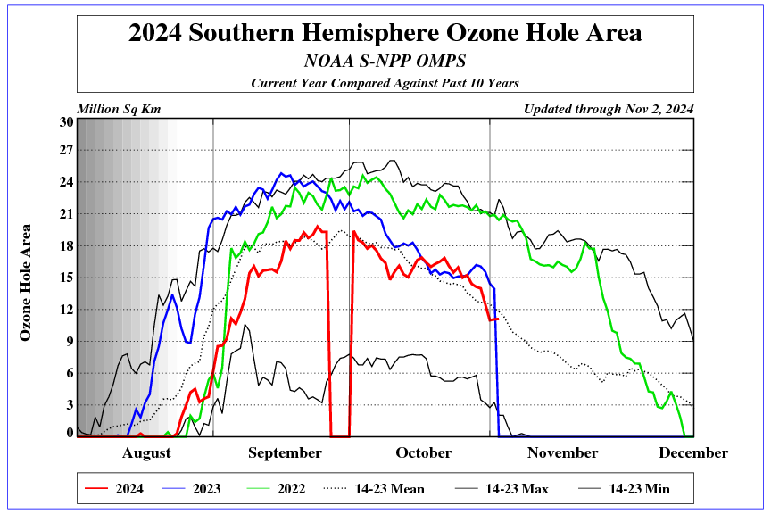
In the northern hemisphere, CO2 levels are rising rapidly due to home heating and the end of the growing season. Will this ensure high winter temperatures? North America seems to be responding poorly to the winter increase in CO2.
That red down at Antarctica is soon to turn blue.
But that blue in both Houses of the U.S. Congress is about to turn red.
I’m hoping the voters throw another tantrum, ala Peter Jennings.
IF the elections are fair your certainly correct. But at this juncture, that is a big IF!
BTW I just got back from voting. Being a on call truck driver I can’t count on being here to vote so I always vote early.
The polling place was only 2.3 miles from my central Indiana home. I walked in and I was the only one voting. Just me and the poll workers.
I really like the system Indiana has now. Upon entering and confirming your identity and registration they issue a paper ballot marked with your vital information.
You place that paper ballot in the machine and through the touch screen menu making your selections. When finished it prints your selections on the paper ballot. You then put the paper ballot into the provided envelope and drop it in the box.
I really like seeing a hard copy of my votes and knowing that the only hacking that could be done would be in the machine that counts and tabulates.
The whole process took 10 minutes.
La Niña will continue until a clear peak in solar activity (a strong increase in solar wind speed over a long period of time).
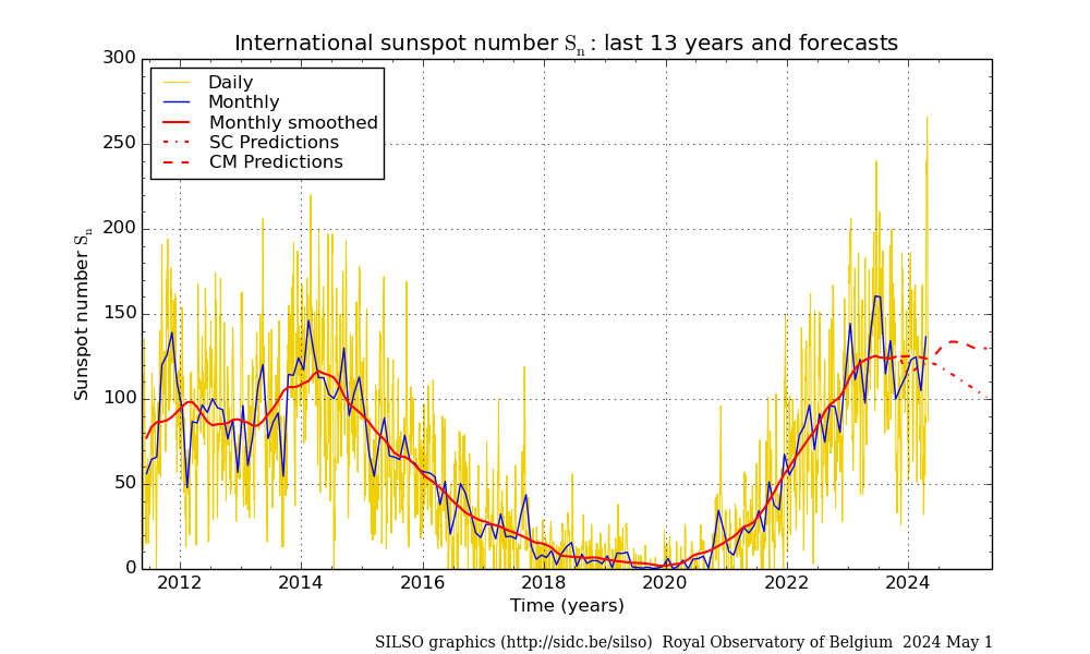
http://www.bom.gov.au/archive/oceanography/ocean_anals/IDYOC007/IDYOC007.202211.gif
Mr Palmowski’s observation is most interesting. Let us see whether he is correct. But a second long Pause would be fatal to the climate Communists.
In other news! Winter Park, considered the top ski resort in the US by many, opened two lifts last weekend. The earliest it has opened in it’s 87 year history. Two other large resorts have also opened!
And there is one heck of a lot more coming out west. The NW US is going to get plastered with snows extending down through California and into Arizona!
It is looking like the US, or at least the western US, is on track to have an excellent ski season just like the Aussies had for their winter this year.
See the current surface temperature trend. A look at the Gulf of Alaska.

Lord Monckton,
Joe Bastardi seems absolutely convinced that the warmer SSTs are being driven by increased geothermal activity along the ring of fire and the mid Atlantic ridge. And that is the source of higher water vapor levels. I was wondering what your thoughts on the subject are?
Rah is quite right to point out Joe Bastardi’s finding. The ranking expert on subocean volcanism, Professor Arthur Viterito, confirms Joe’s analysis. In a normal scientific domain, a simple experiment would be conducted, by which – particularly in the Nino 3-4 region of the tropical Eastern Pacific, where the rate of tectonic divergence driven by magmatic intrusion is an order of magnitude more rapid than anywhere else on the planet – ocean-floor temperatures along the ridges would be continuously monitored.
But such measurements might suggest that variability in subocean volcanism is the chief cause – or, at any rate, a significant cause – of global warming. And that does not fit the Party Line, so the experiments are not funded by the gatekeepers.
The plume from the Tonga eruption reached 57 km. That is into the mesosphere and thus was considerably more powerful than Pinatubo. Think if the tremendous energy released before it reached the surface!
More misleading attacks on climate models from Monckton of Baloney
The IPCC wild guess called ECS are for several centuries from now. The less radical wild guesses for TCS are for the next 70 years. Any comparison of observations and IPCC wild guesses should focus on TCS. In addition, it would be more accurate to use RCP 4.5 rather than RCP 8.5, which is unrealistic. When using TCS and RCP 4.5, the IPCC models would appear to be reasonable. A smarmy Climate Howler named Zeke H. did just that to “prove” the IPCC models were “accurate”.
Model predictions for TCS using RCP 45 may appear tpo be reasonable guesses, but the IPCC goal is to scare people, so they “sell the public” ECS with RCP 8.5 == their worst case wild guess of the climate in several centuries, rather than a reasonable best case wild guess using TCS and RCP 4.5
The latest IPCC guesses:
In several centuries (ECS in AR6): +2.5 to +4.0 degree C.
In 50 to 100 years (TCS in AR6): +1.4 to +2.2 degree C.
Mr Greene here repeats his ill-informed inaccuracy from upthread. If he were to ask his kindergarten mistress to read him page xxiv of IPCC’s 1990 First Assessment Report, he would learn – or, at any rate, hear – that IPCC itself predicted 1.8 K warming from preindustrial times to 2030; but 0.45 K warming had already occurred up to 1990, so that the medium-term prediction was indeed 1.35 K warming from 1990-2030, or about a third of a Kelvin per decade in the medium term. Only a seventh of a Kelvin per decade has occurred since.
In 1990, as in 2021, IPCC’s midrange long-term prediction of warming (ECS) was 3 K. However, given that the transient warming predicted almost a third of a century ago has proven to be little more than 40% of what was then confidently predicted, it is by no means illegitimate to conclude that just as transient or medium-term sensitivity (TCS) was greatly overstated so the long-run sensitivity (ECS) may likewise have been overstated.
CMoB said: “ If he were to ask his kindergarten mistress to read him page xxiv of IPCC’s 1990 First Assessment Report”
It is you that needs to read the IPCC’s 1990 First Assessment Report. It is right there on pg. xxiv. You picked scenario A (Business-as-Usual) even though there were 3 other scenarios B, C, and D with scenario C better representing the choices humans actually made. And because you’ve been told about this multiple times there is no other plausible explanation for your continued misrepresentation than one of intentional deceit.
How’s scenario C getting along?
Scenario C is the scenario closest to matching the emission pathway humans actually choose. It shows 0.55 C of warming from 1990 to 2020. A blend of HadCRUTv5 and UAH shows +0.56 C of warming over the same period. It’s not quite perfect, but it’s pretty close.
So, a completely underwhelming rate of warming. Might as well give up all the hysteria about CO2, yes?
I don’t know if it is underwhelming or not. And it doesn’t really matter because even if it was it does not justify Monckton’s misrepresentation of it.
It is the furtively anonymous “bdgws” who is misrepresenting matters. CO2 emissions have very considerably exceeded IPCC’s 1990 business-as-usual scenario.
“It is the furtively anonymous “bdgws”
Cloud yelling. He told you his name at least twice that I can recall. WUWT is full of non de WUWT’s. Most of whom are better at it than us. bdgwx just blurted his name out and I have given my Oklahoma Professional Petroleum Engineering Registration number out twice. 30 seconds of clever searching would out me.
I could tell blob showed up to support his fellow trenders…
Nonsense. The emissions trajectory is well above IPCC’s business-as-usual scenario, which envisioned holding emissions at their 1990 level. Other scenarios involved cuts in emissions. Annual CO2 emissions are about 50-60% above their 1990 level.
CMoB said: “The emissions trajectory is well above IPCC’s business-as-usual scenario”
You think that CO2 was > 440 ppm in 2020?
You think that CH4 was > 2500 ppb in 2020?
You think that CFC11 was > 325 ppt in 2020?
And YMS—yet more spam.
Scenario A is the one on which IPCC should be judged because it is the business-as-usual scenario, and emissions have exceeded IPCC’s 1990 business-as-usual scenario.
CMoB said: “emissions have exceeded IPCC’s 1990 business-as-usual scenario”
You think that CO2 was > 440 ppm in 2020?
You think that CH4 was > 2500 ppb in 2020?
You think that CFC11 was > 325 ppt in 2020?
A while back I had an exchange with someone (I forget who, it may even have been “Richard Green”) where I referenced Figure A.9 of the FAR, which can be found on page 336 (in the “Annex”).
Comparing both the page xxiv option and Figure A.9 with actual GMST numbers gives the following figure.
NB : With my computer setup I can only add one image file from my local disk per WUWT comment.
Just plotting the (1979 to 2021) trend lines highlights the divergence of the FAR’s “projections” with reality.
For reference, FAR Figure A.9, including its caption.
That’s pretty cool. Can you add a line for FAR “C”?
No point in looking at scenario C. It was scenario A that was closest to what has been observed since 1990. In that scenario, it was envisioned that CO2 concentrations would be held at their 1990 levels. That did not happen: they are now 50-60% above their 1990 levels.
Sorry, but I think you are conflating the IPCC FAR with Hansen et al 1988, which had a “Scenario C” with CO2 levels held constant from the year 2000 onwards (at 368 ppm).
The “projections” for various GHGs in the IPCC FAR can be seen in Figure 5, on page xix of the “Policymakers Summary” (or SPM, as we would now say).
The IPCC FAR‘s “Scenario C” has CO2 levels rising (relatively slowly) to ~500 ppm in 2100.
CMoB said: “No point in looking at scenario C. It was scenario A that was closest to what has been observed since 1990.”
You think CO2 was 440 ppm in 2020?
You think CH4 was 2500 ppb in 2020?
You think CFC11 was 325 ppt in 2020?
More bgwxyz spam…
Yes, but note that these graphs are all derived from “zoom in and hold up a transparent ruler to the computer screen” calculations.
Even though I check the “all the way to 2100” shapes look (at least) “similar” to the originals, they are strictly at the “interested amateur” level.
– – – – –
There is another WUWT article about the media (and the IPCC, and others) hyping up the climate “crisis”.
When people look back at the legacy of the FAR, how many times do they mention “Business as Usual (BaU)” and how many times do they talk about “Scenario C” ?
Mark BLR said: “Yes, but note that these graphs are all derived from “zoom in and hold up a transparent ruler to the computer screen” calculations.”
Yeah. I know. It’s a lot of work, but much appreciated.
Mark BLR said: “When people look back at the legacy of the FAR, how many times do they mention “Business as Usual (BaU)” and how many times do they talk about “Scenario C” ?”
Probably a lot…especially here on WUWT. That’s why we need to educate people.
HAHAHAHAHAAHAHAHAHAHAAH!
[ Wince … ]
You were doing so well up to there.
I am trying to inform people with what can be, at best, described as my “idle musings” or “spreadsheet graffiti”.
I have even occasionally qualified my comments in the past with something along the lines of :
“NB : It is always possible that I might be wrong !”
When was the last time you typed something like that before hitting the “Post Comment” button ?
I have been wrong more often than I can count. That doesn’t change the fact that I’ve yet to see Monckton mention the other scenarios in his pause articles or any article he’s written for that matter. Educating people that these scenarios exist isn’t what I describe as a taboo cause.
You forgot to spam your IPCC graphs for the fiftieth time.
La Nina is now strengthening and will remain for many months, or perhaps another year? That would be a disaster in many parts of the world.
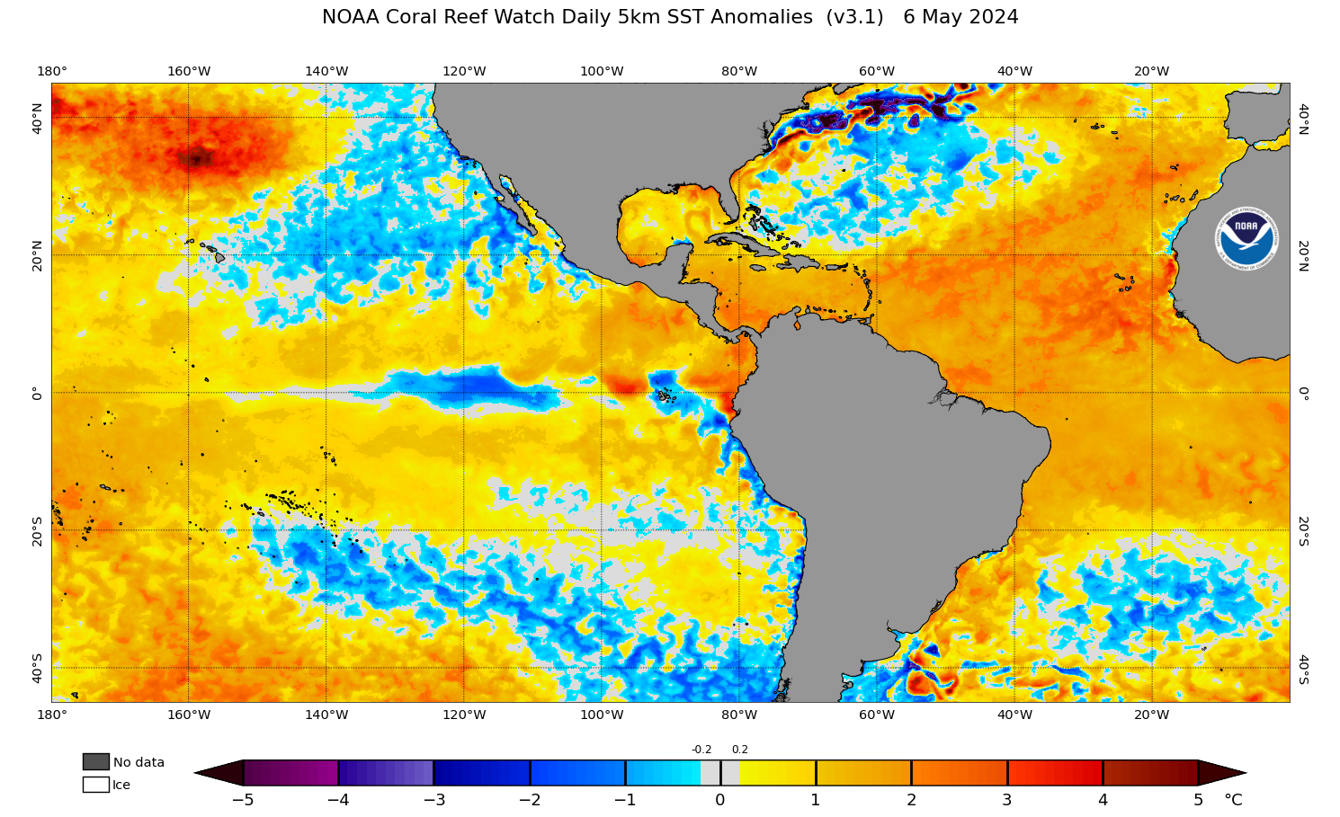
Notice where the warm spots are. It is a system trying to achieve a balance it can never obtain. Every jump in the UAH global temperature set corresponds to increased SSTs at places along the Ring of fire.
Joe Bastardi goes through it, looking back through the years in his last Saturday Summary video. Scroll down to the free video:
WeatherBELL Analytics
The question arises: do the increases in subocean volcanism occur merely randomly, or is there an identifiable causative agent? For instance, is the interaction between the Earth’s mantle, the orbit of the Moon and the motion of the Sun about the gravitational barycenter of the solar system contributing to additional flexing of the tectonic plates? So far, I have not seen an answer to that question.
Arthur Viteriro has several papers on that matter, although I remain skeptical.
Even though even the UN admits that the ENSO cycles are not a result of “climate change” caused by increased CO2 levels, you know darn well that when the disasters come it will be “global warming” that will be screamed by every major media source.
Lord Monckton
You write
“China has also been quietly buying up lithium mines and processing plants all over the world. When I recently pointed this out at a dinner given by a U.S. news channel at London’s Savoy Hotel, a bloviating commentator who was present said that Britain would be all right because we had a large deposit of lithium in Cornwall. “Yes,” I snapped back, “and China owns 75% of that mine.” The bloviator had no idea.”
I live in next door Devon so hear frequent references to the Cornish mine but never to the Chinese connection. Do you have a reference for that please?
tonyb
In response to Tony B, it was reported in the Daily Telegraph in December 2021 that China was acquiring Cornwall’s largest lithium mine, and that the Government – at that time wholly unaware of the threat posed by China’s dominance not only in lithium carbonate and lithium hydroxide production but also in other rare metals such as neodymium – did nothing to hinder the acquisition, as far as I can discover.
I have read about the Chinese takeover of a British lithium mining company (Bacanora) but I don’t believe they run any mines in Cornwall. Perhaps the good lord could provide more information, if there is any?
Your Lordship appears to be the only peer of the realm that has his head screwed on correctly. Sadly, the rest of them seem hell bent on the destruction of the country.
https://committees.parliament.uk/publications/30146/documents/174873/default/
None of this has anything to do with science, the environment or “saving the planet”, it’s all about forcing us plebs into smaller, shorter, more miserable lives. Do you think any of them will adopt the “behavioural changes” proposed for the rest of us?
The Right-Handed Shark is correct: Their Lordships would not dream of inflicting upon themselves the miseries they wish the mere proletariat to endure.
The long-term forecast shows the division of the polar vortex in the lower stratosphere into two centers in line with the geomagnetic field to the north.

Huh? It was the Ukrainian Russians who were being massacred by the Ukie Nazis…
In Donbas (from 2014-22, i.e. 8 years), officially recognised and verified deaths of at least 3,901 civilians, about 4,200 Ukrainian servicepersons, and about 5,800 Russian-backed militants.
From Feb-Oct this year (i.e. 8 months) the UN has registered 6,430 civilians killed and 9,865 injured. Those totals are only provisional and will undoubtedly end up being much, much higher.
Who is doing the massacring?