Guest Post by Willis Eschenbach
Through what in my life is a typical series of misunderstandings and coincidences, I ended up looking at the average model results from the Climate Model Intercomparison Project 5 (CMIP5). I used the model-by-model averages from each of the four scenarios, a total of 38 results. The common period of these results is 1860 to 2100 or some such number. I used the results from 1860 to 2020, so I could see how the models were doing without looking at some imaginary future. The CMIP5 analysis was done a few years ago, so everything up to 2012 they had actual data for. So the 163 years from 1860 to 2012 were a “hindcast” using actual forcing data, and the eight years from 2013 to 2020 were forecasts.

Figure 1. CMIP5 scenario averages by model, plus the overall average.
There were several things I found interesting about Figure 1. First was the large spread. Starting from a common baseline, by 2020 the model results ranged from 1°C of warming to 1.8°C of warming …
Given that horrible inter-model temperature spread in what is a hindcast up to 2012 plus eight years of forecasting, why would anyone trust the models for what will happen by the year 2100?
The other thing that interested me was the yellow line, which reminded me of my post entitled “Life Is Like A Black Box Of Chocolates“. In that post I discussed the idea of a “black box” analysis. The basic concept is that you have a black box with inputs and outputs, and your job is to figure out some procedure, simple or complex, to transform the input into the output. In the present case, the “black box” is a climate model, the inputs are the yearly “radiative forcings” from aerosols and CO2 and volcanoes and the like, and the outputs are the yearly global average temperature values.
That same post also shows that the model outputs can be emulated to an extremely high degree of fidelity by simply lagging and rescaling the inputs. Here’s an example of how well that works, from that post.

Figure 2. Original Caption: “CCSM3 model functional equivalent equation, compared to actual CCSM3 output. The two are almost identical.”
So I got a set of the CMIP5 forcings and used them to emulate the average of the CMIP5 models (links to models and forcings in the Technical Notes at the end). Figure 3 shows that result.

Figure 3. Average of CMIP5 files as in Figure 1, along with black box emulation.
Once again it is a very close match. Having seen that, I wanted to look at some individual results. Here is the first set.

Figure 4. Six scenario averages from different models.
An interesting aspect of this is the variation in the volcano factor. The models seem to handle the forcing from short-term events like volcanoes differently than the gradual increase in overall forcing. And the individual models differ from each other, with the forcing in this group ranging from 0.5 (half the volcanic forcing applied) to 1.8 (eighty percent extra volcanic forcing applied). The correlations are all quite high, ranging from 0.96 to 0.99. Here’s a second group.

Figure 5. Six more scenario averages from different models.
Panel (a) at the top left is interesting, in that it’s obvious that the volcanoes weren’t included in the forcing for that model. As a result, the volcanic forcing factor is zero … and the correlation is still 0.98.
What this shows is that despite their incredible complexity and their thousands and thousands of lines of code and their 20,000 2-D gridcells times 60 layers equals 1.2 million 3-D gridcells … their output can be emulated in one single line of code, viz:
T(n+1) = T(n)+λ ∆F(n+1) *(1-exp( -1 / τ ))+ ΔT(n) exp( -1 / τ )
OK, now lets unpack this equation in English. It looks complex, but it’s not.
T(n) is pronounced “T sub n”. It is the temperature “T” at time “n”. So T sub n plus one, written as T(n+1), is the temperature during the following time period. In this case we’re using years, so it would be the next year’s temperature.
F is the radiative forcing from changes in volcanoes, aerosols, CO2, and other factors, measured in watts per square metre (W/m2). This is the total of all of the forcings under consideration. The same time convention is followed, so F(n) means the forcing “F” in time period “n”.
Delta, or “∆”, means “the change in”. So ∆T(n) is the change in temperature since the previous period, or T(n) minus the previous temperature T(n-1). Correspondingly, ∆F(n) is the change in forcing since the previous time period.
Lambda, or “λ”, is the scale factor. Tau, or “τ”, is the lag time constant. The time constant establishes the amount of the lag in the response of the system to forcing. And finally, “exp (x)” means the number 2.71828 to the power of x.
So in English, this means that the temperature next year, or T(n+1), is equal to the temperature this year, T(n), plus the immediate temperature increase due to the change in forcing, λ F(n+1) *(1-exp( -1 / τ )), plus the lag term, ΔT(n) exp( -1 / τ ) from the previous forcing. This lag term is necessary because the effects of the changes in forcing are not instantaneous.
Curious, no? Millions of gridcells, hundreds of thousands of lines of code, a supercomputer to crunch them … and it turns out that their output is nothing but a lagged (tau) and rescaled (lambda) version of their input.
Having seen that, I thought I’d use the same procedure on the actual temperature record. I’ve used the Berkeley Earth global average surface air temperature record, although the results are very similar using other temperature datasets. Figure 6 shows that result.

Figure 6. The Berkeley Earth temperature record (left panel) including the emulation using the same forcing as in the previous figures. I’ve included Figure 3 as the right panel for comparison.
It turns out that the model average is much more sensitive to the volcanic forcing, and has a shorter time constant tau. And of course, since the earth is a single example and not an average, it contains much more variation and thus a slightly lower correlation with the emulation (0.94 vs 0.99).
So does this show that forcings actually rule the temperature? Well … no, for a simple reason. The forcings have been chosen and refined over the years to give a good fit to the temperature … so the fact that it fits has no probative value at all.
One final thing we can do. IF the temperature is actually a result of the forcings, then we can use the factors above to estimate what the long-term effect of a sudden doubling of CO2 will be. The IPCC says that this will increase the forcing by 3.7 watts per square meter (W/m2). We simply use a step function for the forcing with a jump of 3.7 W/m2 at a given date. Here’s that result, with a jump of 3.7 W/m2 in the model year 1900.

Figure 7. Long-term change in temperature from a doubling of CO2, using 3.7 W/m2 as the increase in forcing and calculated with the lambda and tau values for the Berkeley Earth and CMIP5 Model Average as shown in Figure 6.
Note that with the larger time constant Tau, the real earth (blue line) takes longer to reach equilibrium, on the order of 40 years, than using the CMIP5 model average value. And because the real earth has a larger scale factor Lambda, the end result is slightly larger.
So … is this the mysterious Equilibrium Climate Sensitivity (ECS) we read so much about? Depends. IF the forcing values are accurate and IF forcing roolz temperature … maybe they’re in the ballpark.
Or not. The climate is hugely complex. What I modestly call “Willis’s First Law Of Climate” says:
Everything in the climate is connected with everything else … which in turn is connected with everything else … except when it’s not.
And now, me, I spent the day pressure-washing the deck on the guest house, and my lower back is saying “LIE DOWN, FOOL!” … so I’ll leave you with my best wishes for a wonderful life in this endless universe of mysteries.
w.
My Usual: When you comment please quote the exact words you are discussing. This avoids many of the misunderstandings which are the bane of the intarwebs …
Technical Notes:
I’ve put all of the modeled temperatures and forcing data and a working example of how to do the fitting as an Excel xlsx workbook in my Dropbox here.
Forcings Source: Miller et al.
The forcings are composed of:
- Well mixed greenhouse gases
- Ozone
- Solar
- Land Use
- Snow Albedo & Black Carbon
- Orbital
- Troposphere Aerosols Direct
- Troposphere Aerosols Indirect
- Stratospheric Aerosols (from volcanic eruptions)
Model Results Source: KNMI
Model Scenario Averages Used: (Not all model teams provided averages by scenario)
CanESM2_rcp26
CanESM2_rcp45
CanESM2_rcp85
CCSM4_rcp26
CCSM4_rcp45
CCSM4_rcp60
CCSM4_rcp85
CESM1-CAM5_rcp26
CESM1-CAM5_rcp45
CESM1-CAM5_rcp60
CESM1-CAM5_rcp85
CNRM-CM5_rcp85
CSIRO-Mk3-6-0_rcp26
CSIRO-Mk3-6-0_rcp45
CSIRO-Mk3-6-0_rcp60
CSIRO-Mk3-6-0_rcp85
EC-EARTH_rcp26
EC-EARTH_rcp45
EC-EARTH_rcp85
FIO-ESM_rcp26
FIO-ESM_rcp45
FIO-ESM_rcp60
FIO-ESM_rcp85
HadGEM2-ES_rcp26
HadGEM2-ES_rcp45
HadGEM2-ES_rcp60
HadGEM2-ES_rcp85
IPSL-CM5A-LR_rcp26
IPSL-CM5A-LR_rcp45
IPSL-CM5A-LR_rcp85
MIROC5_rcp26
MIROC5_rcp45
MIROC5_rcp60
MIROC5_rcp85
MPI-ESM-LR_rcp26
MPI-ESM-LR_rcp45
MPI-ESM-LR_rcp85
MPI-ESM-MR_rcp45
What! No solar activity forcing?
In the voice of Arnold Schwarzenegger, “No, it’s kah-bun.”
I envisage Ol Sol peeping up over the horizon every morning and spying the latest climate equation, which gives him a good laugh to start his day’s work.
He probably has another chuckle about climate equations before he shuts up shop for the day, knowing there will be a new one tomorrow morning to keep the comedy coming.
Because –
“That lucky old sun
has nothin’ to do
but rolll around heaven all day”
Absolutely, sun is the big dog, insolation energy + GCR control valve. Its minor detructor is the Earth itself via magnetic field and volcanic eruptions. Four variables none predictable, but all within a reasonably well defined range, keeping the planet’s climate relatively stable on the centenary to millennial range. On longer time scale Milankovic cycles and possibly galactic transit come to force.
Fortunately for us, the Sun never shuts up shop for the day.
Thanks, Leif. Actually, the solar forcings are included. The total forcings are
WMGHG
Ozone
Solar
Land_Use
SnowAlb_BC
Orbital
TropAerDir
TropAerInd
StratAer
I’ve added that to the head post in the technical notes.
w.
Thanks.
But the ‘solar forcing’ does not match the modern sunspot record.
IMO, it does. Just not immediately.
The LIA was characterized by repeated solar minima.
The Medieval and Modern Warm Periods, and their antecedants, ie the Holocene Climatic Optimum, Egyptian, Minoan and Roman WPs, enjoyed solar maxima.
But I liked your initial comment.
The minima back then were not any deeper than now.
The radiation we get from the sun (TSI) is determined as the sum of dark sunspots and bright magnetic background fields. The latter dominates and overwhelm the sunspots. With no sunspots, it is very possible that TSI was higher during the LIA than now…
But TSI doesn’t rule.
What matters is UV flux.
which is 10 times smaller…
Yet UV effect isn’t just energy, but quality of effect. It makes and breaks ozone and rule air ptessure, influencing the trade winds, which account for ENSO fluctuations.
Ten times on average, but it swings wildly.
Almost certainly not, but it doesn’t matter. What does matter is UV flux.
Now that thar’ is funny.
Hi doc
.. and why would anyone expect that the single partly subjective visual assessment (modern or historic) of one of a number of aspects of the solar activity, would always be a dominant factor of the planet’s climate quasi periodic oscillations.
lots of people expect that…
Thanks, Leif. I hadn’t looked closely at the solar forcing because it’s so tiny … but you’re right.
Most curious … no idea what they’ve done.
w.
Right now you can see on satellite how important a single geographic feature like the Isthmus of Tehuantepec can be to global climate. Positioning of the oceans/continents is one of the primary forcings, some of these others are noise.
If we want to really experiment with geoengineering wouldn’t the be all and end all (likely “end all”) be to open the ithsmus of Panama?
Biggest earth moving project in history, completely alter ocean currents just to see what could happen?
What could go wrong.
Are you saying that the canal did that already? Any references, sorry if it it sounds like a rude challenge or something, but the canal is tiny in comparison to the landmasses around it.
The global warming panic, the climate emergency that is driving people batty is built on a lousy 1-2°C warming over the past ~200 years which is similar to the swing in temperatures from previous warm or cold periods, so basically, situation normal on planet Earth, regardless of the Panama Canal.
Now, if you were talking about REALLY opening wide the Isthmus of Panama so a significant opening is created, enough to affect weather and climate, well that would be interesting to talk about!
I thought there was a difference in sea levels between the 2 sides . . could stick a few turbines in the flow and global energy problem solved.
Easy
Solar forcing is coupled with clouds.
As Willis E well has described.
Solar brightening and solar dimming is a fact and not well explained.
We have 20% more sun(h) today compared to 1980
Nice job, Willis. Like many WUWT denizens, I look forward to your articles, and I learn a lot from them.
I also learn quite a bit from the responses, even the critical ones. Some responses make me think. Some responses make me think the author is a pretentious prat. Takes all kinds.
Hope your back feels better soon.
Somehow models supposed to be skillful and fit for policy purposes out to AD 2100 missed the past six years’ global cooling and the 1998-2014 Pause.
Thus, 21st century warming was due to Super El Niño of 2015-16.
Indeed warming since the 1977 PDO shift is largely the story of three Super Los Niños, ie 1982-83, 1997-98 and 2015-16. And they are driven by solar variations.
https://www.sciencedaily.com/releases/2021/04/210405075853.htm
https://aip.scitation.org/doi/abs/10.1063/1.4930679?journalCode=apc
https://journals.ametsoc.org/configurable/content/journals$002fatsc$002f69$002f10$002fjas-d-12-0101.1.xml?t:ac=journals%24002fatsc%24002f69%24002f10%24002fjas-d-12-0101.1.xml
https://www.issibern.ch/teams/interplanetarydisturb/wp-content/uploads/2015/01/Asikainen_03_2014.pdf
Yes! That’s exactly what the more impartial satellite temperature record looks like: step change in temps after an El Nino followed by steady periods – not something expected from steady CO2 increases.
“That same post also shows that the model outputs can be emulated to an extremely high degree of fidelity by simply lagging and rescaling the inputs.”
We’ve been through this before. The forcings are not the inputs to the models. They are deduced from the outputs, or possibly from some intermediate steps. The “one single line of code” is very close to what was used to calculate F. So of course the output temperatures “follow” the forcings. It is just using the formula by which they were deduced in reverse.
“The forcings are not the inputs to the models. They are deduced from the outputs, or possibly from some intermediate steps.”
No? Then what are the inputs?
Gas concentrations, as per scenario. Plus, of course, aerosols, insolation, etc.
“Gas concentrations, as per scenario.”
Like CO2 and CH4? What’s the difference between inputting a forcing in terms of w/m^2 and inputting a change in gas concentration that the GCM, or some subroutine thereof , will directly convert to w/m^2?
“What’s the difference between inputting a forcing in terms of w/m^2 and inputting a change in gas concentration that the GCM”
The important difference is that the former is not done. The reason is that it can’t be. The forcing cited here is a global aggregate. What a GCM needs is a distribution to determine each cell value. With gases you can do that, because they are well-mixed. Maybe not perfectly, but any corrections needed are small. A number for global aggregate forcing can’t provide cell values.
Yes, but the gas concentrations are easily convertible to forcings, eg 2XCO2 = 3.7 W/m2, etc. using the IPCC formulas from Myhre et al 1988. And in fact, if we use the historical GHGs specified in the scenarios, we get the forcings I used.
Next, I don’t think the models are using their own internal physics and parameters to determine say the forcings from the change in snow albedo due to black carbon …
Next, I’ve used one set of forcings for all of the models, and gotten extremely good results. This is despite the fact that you are correct that each model is using slightly different forcings.
Finally, it’s a black-box experiment, so the direction of causation doesn’t matter in the slightest. It doesn’t make any difference whether the forcings are being calculated from the temperatures or the temperatures are being calculated from the forcings. The point, and the surprising fact, is that despite the insane complexity of the models, the two are inter-calculable by means of a simple one-line equation.
Thanks,
w.
Let me note also that the MAGICC program is used to emulate the models … and it uses specified forcings.
w.
Nick is playing the usual deflection games .. ignore him.
A further note. There’s a discussion here of the GISS CMIP5 model runs. In that it is clear that many of the forcings are NOT calculated by the model, as Nick states, but are calculated externally and imposed on the model.
w.
” In that it is clear that many of the forcings are NOT calculated by the model”
No, the link (Miller et al) makes clear that they are. Here is their familiar plot of forcings
And here is what they say about how the plot was calculated.
In Table 2 they even list the model runs that were used.
Nick, in the MAGICC model, the following radiative forcings are calculated outside the model:
Black carbon-burning
Black carbon-industrial
Black carbon snow albedo
Landuse
NOx
Organic carbon-burning
Organic carbon-industrial
SOx
Volcanic
Solar
The rest (well-mixed greenhouse gases) are input as emissions.
Again I say, the point is that you can use a one-line equation that is physically well-grounded to calculate the model output from the radiative forcing, or the other way around.
w.
DATA
Yes, but MAGICC is not a GCM. It is a simple model using hemispheric averages. So it doesn’t help your contention that “(GCM) model outputs can be emulated to an extremely high degree of fidelity by simply lagging and rescaling the inputs”.
Thanks, Nick. You are still missing the point.
The point is the extremely simple relationship between the forcings and the temperatures. This is unexpected, whether the forcings are specified a priori or the emissions are specified a priori.
Take CO2 as an example. Yes, you are right that the models use CO2 emissions rather than CO2 forcing as their input. But the atmospheric concentration is easily calculated from the emissions, and the forcing is easily calculated from the atmospheric concentration.
But let’s assume that both the forcings and the temperatures are totally the output of the models, and are not calculatable without them. We know that’s not true because e.g. CO2 forcing is calculatable from emissions, but for the sake of discussion.
It is STILL surprising that such a bog-simple relationship exists between forcings however calculated and model temperatures.
I’m taking another look at this question, and I’ll post up on it when done.
Finally, thanks for all of your comments here. They push me to reconsider my own assumptions and conclusions, which is always a good thing.
w.
Top notch job as always! Love it when I see a new article from you is posted on WUWT.
If it is purely circular in construct, then why does the CMIP model ensemble average run 1.5ºC to 3.0ºC higher than the emulation Willis shows here?
hint: I know the answer. Are you willing to admit it Nick?
This is how it so often goes here:
“Look how a forcing formula emulates temperature so well!”
“But that is because forcings were calculated from that formula”
“So why does the formula emulate temperature so badly?”
In fact Willis’ formula determines temperature differences. It does not determine the offset.
“Look how a forcing formula emulates temperature so well!”
“But that is because forcings were calculated from that formula”
“So why does the formula emulate temperature so badly?”
PS – I see you’re getting downvotes. For the record, I appreciate your willingness to debate the issues on WUWT, but understand why some might find your responses a bit slippery.
I do, too. Nick’s comments are important to this blog, IMHO.
“Who said this?”
Me
“Again, who said this?”
Joel: “why does the CMIP model ensemble average run 1.5ºC to 3.0ºC higher than the emulation Willis shows here?”
Nick Stokes February 3, 2022 11:06 am
Whoa, whoa, back up. Up above you said the forcings were calculated by unknown processes within the climate models.
Now you’re claiming the forcings were calculated from the formula.
Pick a story and stick to it, please.
w.
I was paraphrasing the to and fro
The smoking gun, so to speak, of why the models run too hot (an ECS 2X to 4X higher than observed) and thus ‘why they fail’ is diagnosed by the lack of observation of the CMIP ensemble predicted mid-tropospheric hotspot. That failed prediction is diagnostic of the fact that all the important water vapor physics of cloud formation and precipitation related to convective heat transport in the models is fudged with hand tuning to get the ECS answer the modellers expect.
They might be able to fool the general public and lapdog media journalist, but they can’t fool Mother Nature (a.k.a. the real world).
“The forcings are not the inputs to the models.”
They effectively are when they’re built into the parameterisations.
This is all devils sitting on the head of a pin. The relevant forcings can be found by asssuming the system is stochastic and fitting a regression model to various observed time series of global average temperature, greenhouse gas concentrations etc. My paper on this was recently rejected by Proc. Roy. Soc. A. because it was “too simple”. Evidently they had never heard of Occam’s Razor. See https://www.amazon.com.au/Fluid-Catastrophe-John-Reid/dp/1527532062 .
The link should be https://blackjay.net.au/measuring-climate-change/
There is a wide range of climate models, from the simplest “0-D energy balance models” to the largest and most complex 3-D AOGCM “climate models”.
You have failed to specify which variant(s) of “the models” you had in mind when you were typing your OP here.
My understanding (which may well be wrong in the details !) is that “the (climate) models” can be classified as either :
1) “Full-blown” 3-D AOGCMs, which use GHG emissions as inputs and then “calculate” atmospheric concentrations as outputs (from which RF values are only a simple algebraic formula away…); or
2) “Models of intermediate complexity”, typically 2-D or 3-D, which use atmospheric GHG concentrations as inputs; or
3) “Simple” climate models, from 0-D to 2-D, which use RF numbers “directly” as inputs.
– – – —
I repeat, “the models” is not limited to “GCMs”.
Instead of Willis’s standard “When you comment please quote the exact words you are discussing” request a famous quote (by Voltaire ?) may well be applicable :
– – – —
PS : I completely agree with this sentiment (by “Frank from NoVA” below).
Reading comprehension is a necessity for this site – Willis is not saying that the models use one line of code, but one gets the same result as all those thousands of lines of code running for hours on supercomputers by using his one formula based on lagging the inputs. Just read the article again, his meaning was plainly indicated and everyone else here got the same idea.
Again we see support for ECS in the range of 1.4ºC to 1.5ºC per CO2 doubling. Turn-off the alarms. There is no climate crisis. As HL Mencken would put it, it’s is an imaginary hobgoblin meant to scare the public in order to concentrate power in the hands of a few.
It’s all bullsh*t.
I’ve seen this time and time and time again. The modelling boffins think they know but what they don’t know (yet) is that they don’t know. Climate is a complex (possibly chaotic), dynamic, non-linear, multi-variate system. The clowns don’t even know what all the damn independent variables are.
The modellers don’t have a frickin’ clue.
All nonlinear dynamic systems are mathematically chaotic (a well defined term with several characteristics including but not limited to sensitive dependence on initial conditions and strange attractors in N-1 Poincare space).
That climate is nonlinear is proven by feedbacks like water vapor.
That climate is dynamic is proven by the fact that feedbacks operate with some time lag.
That is just not true. Firstly it is easy to show that no two dimensional system can be chaotic. Secondly there are plenty of nonlinear systems that are strongly dissipative and thus are not chaotic since all trajectories will evolve to some fixed point. Then even if you restrict yourself to driven dissipative systems then often chaos can only be found in restricted parameter regions. The Lorenz system for example is only chaotic for a restricted set of parameter values.
Alright, if it is easy, it shouldn’t be asking too much for you to show it.
It’s hard to show you from flat land.
It is an immediate consequence of the Poincare-Bendixson theorem which was proved in 1901. Have a look on wikipedia.
I’m not very bright so I was hoping that you could explain it in a manner that I could understand, not just provide a link.
Were you perhaps referring to the statement, “However the theorem does not apply to discrete dynamical systems, where chaotic behaviour can arise in two- or even one-dimensional systems.”?
Clyde,
The simple non technical answer is that there is just not enough room in 2 dimensions for chaos to occur.
A 2D dynamical system is defined by a set of equations (dx/dt = f(x,y), dy/dt=g(x,y)) where f and g are smooth continuous functions. There is thus a single trajectory that passes through any point and so in phase space (x,y) trajectories cannot cross.
Thus in 2D, trajectories correspond to paths you can draw on a piece of paper that never self intersect. Now try to draw a curve that remains inside a finite square is smooth (i.e. no sharp turns) and which never crosses itself. If you do this you will see that either the curve approaches a fixed point or a periodic orbit. There is no other option.
The only other option is that your curve goes off to infinity.
In 3D the situation becomes different since when a curve comes close to self intersection it can swerve around itself in the 3rd dimension.
Adding additional
dimensions to a problem allows new dynamics to arise. In 1D for example solutions to d x/d t = f(x)
can not be periodic and must either go to infinity or
to a fixed point.
Am I to assume that this is an example of chao in 2 dimensions since even a double pendulum swings in a plane?
Mike,
That is a 4 dimensional system. There are 4 degrees of freedom — the angle of each pendulum and its velocity. Thus the motion can be chaotic.
He is playing stupid word games like Nick Stokes does with “dimension” he is using the mathematical version.
He’s using the correct version. Chaos requires at least three degrees of freedom.
How is this any different than the ocean or the atmosphere? Neither of these are 2 dimensional. In both you have at least x, y, z, and t (time) as dimensions.
no two dimensional system can be chaotic.
But thin films can – don’t forget the Belousov-Zhabotinski reactions. Plenty of chaos and emergent pattern there. There’s a large literature on chaotic and fractal dynamics in thin films, e.g.
https://www.sciencedirect.com/science/article/abs/pii/003040189190037E
https://iopscience.iop.org/article/10.1088/1742-6596/1141/1/012004/meta
You can hardly deny that turbulence – that is, high dimensional chaos, is not a prominent, even dominant feature of ocean circulation, which is where climate comes from (in case you were wondering).
https://earth.nullschool.net/#current/wind/surface/level/orthographic=-345.00,0.00,128
But what is more interesting than chaos per se in climate is where chaos decreases in dimensionality from turbulence toward borderline chaos, the regime where the interesting emergent spatiotemporal patterns and oscillations arise.
Two things can give chaotic climate fluid flow systems the dimensional haircut that brings them toward the borderline chaos regime of emergent pattern: internal feedbacks, and external periodic forcings. There are plenty of these both in the earth system.
Ocean driven oscillations based on oceanic feedbacks (often associated with upwelling or downwelling) together with astrophysical forcing include the ENSO on short time scales and “stadium wave” oscillations such as PDO and AMO on longer ones.
https://ptolemy2.wordpress.com/2021/11/13/climate-pandemonium/
Phil,
Looking at the papers you cite. For the first the system is three dimensional not two and so chaos is possible. The second paper describes solving a nonlinear partial differential equation which has an infinite number of degrees of freedom and so again doesn’t count.
I am not denying that nonlinear dynamics plays an important role in lots of areas. Again my point was that the fact that a system is nonlinear does not imply that it is chaotic. There are a lot of nonlinear systems out there that are not chaotic. Just as there are a lot that are.
“Firstly it is easy to show that no two dimensional system can be chaotic”
So there are 3 and 4 dimensional (Gravity and EM ) non-linear chaotic systems and analysis which don’t exist according to you.
So you are clearly using special Izaak Walton physics and probably you need to take that dribble to a physics forum.
LdB,
Giving an example of a 3 or 4 dimensional system that is chaotic does not disprove the claim that 2 dimensional systems cannot be chaotic.
Exactly what in the system we know as Earth is two-dimensional?
“Firstly it is easy to show that no two dimensional system can be chaotic.”
What kind of strawman is this?
You know the context in which the statement was made, right?
You’ve got me there. Non-linear implies > 1 dimension, and dynamic implies another.
The Earth and the biosphere are at least 4 dimensions.
It’s worse than you think. The temperature anomalies that the models are ‘tuned’ to hindcast are based on spatially sparse temperature records that have been heavily tampered to show warming since the onset of the industrial era.
THIS a 1000 gazillion times
What happens when they have to “correct” the past temperature record upon which their hindcasted models are based?
Heck, even if it were 5°C per doubling CO2, it wouldn’t be a bad thing. W.E. has given good evidence that tropical temperatures won’t change much which supported by IPCC as well, so warmunists have no case. And a much warmer north polar region would be a gift to the biosphere there, regardless of any rising of water levels – the extra water is much needed in the biosphere elsewhere. The south polar region would barely notice I think, though the penguins would appreciate the improvement in their living conditions and survival rates.
Anyways, historically the Earth has been warmer than now on average, and it’s insanity to think we could stop it returning to that level.
“T(n+1) = T(n)+λ ∆F(n+1) / τ + ΔT(n) exp( -1 / τ )”
Isn’t the ability to emulate the output of the “complex” GCMs as a simple function of the “forcings” similar to Pat Frank’s findings? If so, would you agree with his conclusion that the models are essentially meaningless because the temperature impact from errors in cloud forcing at all time scales far exceeds the modeled change in surface temperature?
A link to “Pat Frank’s findings” would be useful here …
Thanks,
w.
One link:
https://wattsupwiththat.com/2019/09/11/critique-of-propagation-of-error-and-the-reliability-of-global-air-temperature-predictions/
Pat and I have differed on some issues, but my admiration for him and his work on error propagation, so devastating to the CACA “consensus”, is unlimited.
PS: The man is fearless and honest as the day is long, traits sorely lacking in the CACA cabal.
Thanks for your kind words, John.
If I recall this past low value discussion, here is error propagation: You can’t keep your car on the road. Because all steering input contain errors. So at any time because of error propagation, you are in the ditch. But here’s the problem with that failed theory. The system feeds back. Everytime something is off you don’t veer into a ditch. Sorry. That’s the way it works.
Another example: There is no life on Earth. Because all errors have led us and everything else to extinction. Life and certain models can feedback to keep things stable enough.
Another example: Goats actually cannot walk on the side of steep mountains. Because every step has an error in it. So they all died centuries ago. Wait, there’s feedback to make up for that.
Not at all comparable to Pat’s work on CACA.
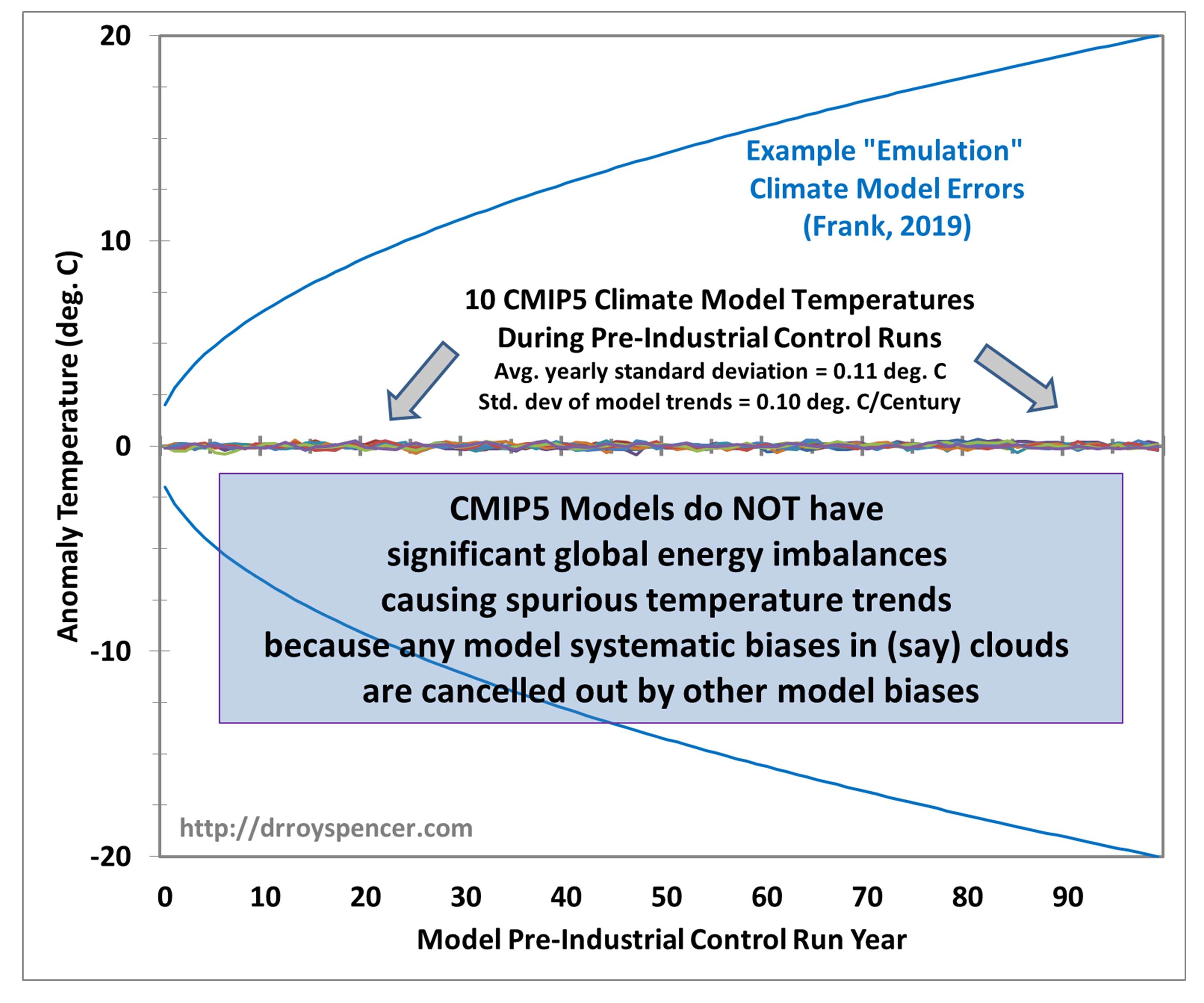
Maybe you’re right. Here’s Spencer: “The reason is that the +/-4 W/m2 bias error in LWCF assumed by Dr. Frank is almost exactly cancelled by other biases in the climate models that make up the top-of-atmosphere global radiative balance. It doesn’t matter how correlated or uncorrelated those various errors are with each other: they still sum to zero, which is why the climate model trends in Fig 1 are only +/- 0.10 C/Century… not +/- 20 deg. C/Century. That’s a factor of 200 difference.”
What I am saying is the models act as if they feedback. For instance, they still disburse El Nino events and recover from huge volacanoes. They feedback like the climate does, like your body does. Like my goat on a mountain does. Spencer says more or less, apply the right math. I predict you can’t keep any car on the road with my Dr. Frank math. Because all steering inputs have errors. Spencer says also, if they didn’t the CMIPs would show like 20 C warming. You might be technically right. But I am on the right path I think.
The map is never the territory.
“I predict you can’t keep any car on the road with my Dr. Frank math. Because all steering inputs have errors”
I think the analogy with driving on a road needs to start with…the road is the path that is unknown.
So imagine driving in a massive car park and making whatever steering corrections you like and then afterwards put in the “road” as the path in that car park and see how well you did driving down it.
It’s almost certain the car quickly left where the road was and went on its own merry way around the car park.
Roy Spencer says the propagation errors don’t occur because there are compensating errors in the models. Oh, so it’s all good then?
No, it’s not! That just makes it so much worse. That is an admission that there so many errors in the model that aren’t even being uncovered and measured.
Ragnaar,
What you describe is how weather forecasting is done with weather models. Weather forecasters make new model runs every 6 or 12 hours using the latest set of observations, that is they are constantly corrected with observables.
This is not how climate modeling is done. Climate models frequently run into the ditch because they rely on estimating non-observables (via parameters and finite precision measured inputs). Those in-the-ditch runs just never see the light of day beyond the trash can in the climate team computer center.
Bad analogies to the issue of error propagation. Taking the first example to illustrate; yes, any competent driver can easily compensate for the tracking error in a typical car, because this error is relatively minor compared to the lock-to-lock range of the car’s steering mechanism. But tell me honestly, would you drive, or allow a loved one to drive, a car in which the steering error was so large that a mere second of driver inattention would allow the car to rapidly veer into the oncoming lane or a concrete bridge abutment? Maybe you or your loved one consider yourselves skilled enough drivers to compensate for the errors of such a defective steering system, but why would either of you voluntarily take the risk?
The fact that a GCM can somehow ‘offset’ errors in cloud cover, the temperature equivalent forcing impact of which far exceeds that of the GHG additions during the same period, against other model errors doesn’t mean these errors don’t matter. While they don’t show up, or rather, are not allowed to cause the model’s temperature outputs to attain clearly unphysical values, they are still inherent to the model, which means that these outputs still have no physical basis no matter how reasonable they may seem.
Frank from NoVA:
It doesn’t happen right away. But it happens. Then we see it happening, and adjust. AI vehicles can do the same thing. But the answer is not you move 1 foot to the right or left every 15 minutes. I am assuming this skill the models have. But if this problem does happen, the accident reports would show us that. When we drive, we iterate. It’s mostly corrections. How about this: The CMIPs model a heat engine. The front end impacts the back end. If a signal from the front end misfires, the thing doesn’t blow up. The back end ramps up once it actually sees what really happened at the front end.
I think the point Pat Frank is making isn’t about errors in the result, its about the propagation of uncertainty that comes about with the errors propagating with each iteration of the model’s run.
Yes, GCMs are constrained to stay within believable results (when they’re not blowing up that is) but the propagation of errors (ie accumulating uncertainty) means that whatever result is returned, its within the propagated error limits which have become enormous.
So the models can return any value they like (they’re tuned to return believable ones) and its within their enormous error range.
It makes any result returned by a GCM utterly useless as a projection.
You pretty much nailed it. The problem with the driving example is that it doesn’t cover the situation where the uncertainty of the input to the steering mechanism is additive. A better analogy would be trying to correct the direction of the car while skidding on ice. Usually any corrections are additive to the amount of skidding, the car just keeps on swapping direction in an ever increasing amount, left and right, till it spins out of control and where you wind up is no longer under your control.
An even better example would a tank slapper wobble on a motorcycle. Once that wobble starts almost anything you do with the handlebars will make it worse till you “slap the ground with your tank”! With each iteration of the wobble whatever you do just makes it worse. (there is one thing you can try but I’m not going to give away the secret here)
I think a clear example would be modelling the tattslotto balls rolling around in their cage. Very quickly the accumulating errors in their modelled positions mean that the modelled results no longer reflect reality and the modelled result won’t be the same as the actual result.
So at any time because of error propagation, you are in the ditch. But here’s the problem with that failed theory. The system feeds back.
========
That is incorrect because the feedback is in the future and not available at the start of the journey.
The models are trying to predict the traffic and potholes on the road in the future using averages from today.
The same problem affects all inertial navigation systems. They need mid course corrections based on future data that is not available in the present.
See the plot:
This is not a plot of the possible GMST outcomes of a CMIP run.
The plot looks like chaotic bifurcations.
Uncertainty is not error!
That plot has nothing to do with error propagation, Ragnaar. It merely shows that Roy Spencer got it completely wrong.
It prima facie conveys an impossibility. Look at the two lines. Roy has them predicting temperatures that coincidentally both rise and fall.
Somehow he didn’t notice that impossibility built right into his figure. And neither did you.
See my analytical comment here: https://wattsupwiththat.com/2019/10/15/why-roy-spencers-criticism-is-wrong/
Here’s another link.
Pondering. Has anyone attempted to construct a GCM without GHG components? Not saying GHGs don’t influence but since none of the current models work all running too hot, why not try to make one the runs too cool? Edison knew 999 ways how not to make a light bulb. He also made a light bulb because of that.
You mean, if someone took a fully parameterized GCM and then zeroed out the future increases in GHG concentrations, would the earth then cool over time? I’ve wondered that myself.
The answer that I will offer to your question is;
Nope, no cooling.
Same end result, Same “ball court” result finale, as all others… a projection, of Atmospheric thermal expansion at ~3C warming equivalent, with a 200-220 ppm CO2 upswing correlation.
But with a Delta Time reaching at some 2K years+ (or even more),instead of decades or a century or two.
The main thing that actual GCM simulations (free of extra extrapolation) diverge from each other, is Time factor. Basically GCM simulations perform and do the same steps and cycles, almost, but in a different delta T.
That is my understanding, which you should not take it for granted…obviously.
cheers
Rob_Dawg-
In Hason’s 1988 paper he ran a 100 year baseline (starting in 1958) with the GHG’s held at constant 1958 values. The results are presented as Figure 1 in the paper. It surprises me that you don’t see this figure quoted more often. If I were more computer savvy, I would include it here, but alas I am not.
Interestingly, the temp anomaly peaks around 2008 and then decreases for the next 30 years.
Today that result would be streng verboten!
Thanks for the reference. It (Figure 1) looks like a random walk. Was the so-called ‘control run’ a single iteration of Hansen’s model or the average of many runs?
old engineer
Technically speaking, GCM(s) do not do either the absence or the constant of GHG’s.
Even when water vapor, the most potent GHG, due to parameterizing could end up and considered constant at some given point… to a given degree.
Eschenbach demonstrates the net forcings factor and constant has no physical basis and is a simple function of the temperature series. An empirical fit with many (unlimited) degrees of freedom. The limit is only bound by the analysts imagination. This statistical relationship has no need for knowledge of mechanisms and so we have learned nothing about how the climate works.
It is irrelevant what anyone may believe about the physics of greenhouse theories or the partitioning of forcings, or what they believe about feedbacks. Radiation budget diagrams are imaginary, like cartoons, and so is anything gleaned from their computational GCMs. The output is merely a series impressive pictures, figments.
Regardless of what anyone believes might be happening the atmosphere has only one degree of freedom, the ratio of absorbed solar to non-radiation flux density. LW radiation equilibrium is not a free variable. The ratio of surface upward flux and OLR has not changed as predicted by current forcing hypotheses, in fact, it has barely changed at all (and in the wrong direction).
“IF the temperature is actually a result of the forcings”
The AMO doesn’t directly follow forcings, it is cooler when the solar wind is stronger and warmer when the solar wind is weaker.
You have basically done a curve fitting using the known data. This is rather easy for any set of data. But how does that curve fit help in predicting the future path? Whether the models are good or bad, that is their function, to try to predict the future.
The fact that curve fitting is easier than writing millions of lines of code is immaterial here. All forecasts have errors, which is why in the real world developing cost functions are important. Whether it’s WE’s emulator, or a GCM, you don’t ‘bet the ranch’ on a forecast unless you can afford the likelihood that it’s wrong.
I am a professional meteorologist and forecaster. I know full well about model error. I have written atmospheric models. We always use them with healthy skepticism. That is what I get paid for. Unlike climate modelers who seem to think their models are truth.
WE, a most interesting analysis. An observation and a question.
The Berkeley Earth result in your last figure is well within the error bounds of the revised Lewis and Curry energy budget method, which also relies on observed past temperatures. So that is in a way an observational triangulation.
The question is why the last figures Model ECS (1.4) is less than half of the CMIP5 average (3.2). My speculation is that Pat Frank’s compounding error issue is a root cause, as the models play out to 2100 and we know from the 8 year predictive results to 2020 that CMIP5 has a built in warm bias from unavoidable parameterization that drags in the natural variation attribution problem. Your method of deriving lambda and tau largely avoids that compounding error issue.
Hey, Rud, glad as always to hear from you. I trust you’re well.
I’m not sure why the ECS value I got was much smaller than theirs. It may be related to the fact that the data I have only rolls out to 2012.
I’m looking at the MAGICC data to see if I can get a longer set of forcings. Not sure the required data is there
w.
Willis
I got stuck for a while on your fig. 6 left panel. The caption says “Berkeley Earth Average Temperature…” and the legend in the figure says “CMIP Average Temperature”. I assume (after pondering it for the duration of a tea break) that the caption is right and that the legend is actually inherited from Fig.3.
Any chance that you could redo this exercise using actual temperatures from the CMIPs rather than anomalies?
I seem to recall another post a few years back saying that you could reproduce the CMIP ensemble with a hand-held calculator. Was it Pat Frank? But just think of the prestige attached to having a supercomputer in your lab! Who cares if it generates meaningful results? It probably impresses the heck out of the graduate students…
As the caption says, the left panel is the Berkeley Earth Average Temperature, and the right panel is the CMIP average temperature. I’ve changed the caption to more clearly reflect this.
w.
I have never received an answer to these questions from any Climate Scare Alarmist: What should the earth’s perfect temperature be and has it ever been and for how long; and what should the correct level of CO2 be and do you believe like some that CO2 is a dangerous pollutant, and most important, if so, who amongst us should be forced to hold our breath to stop CO2 from getting into the atmosphere???(considering that we inhale 400ppm and exhale approximately 20,000ppm)
Last but not least, is there a published or otherwise empirical paper or experiment linking CO2 to the Earth’s temperature? I think
NOT.
ALSO
To my limited knowledge the last glaciation ended about 12,000 years ago and according to scientific records the earth’s temperature has been declining (negative trend line) with a number of ups and downs ever since and will continue to do so until the next glaciation.
Anyone think we can stop it?
I read this blog for fun and education,. I am 77 years old and as yet no one can answer my questions. If given the chance I would love to confront Mann, Kerry, Gore,et all
“ What should the earth’s perfect temperature be and has it ever been and for how long; and what should the correct level of CO2 be and do you believe like some that CO2 is a dangerous pollutant, and most important, if so, who amongst us should be forced to hold our breath to stop CO2 from getting into the atmosphere???(considering that we inhale 400ppm and exhale approximately 20,000ppm)”
Good luck
I understand John Tyndall was the first to demonstrate the ‘greenhouse effect’ in a laboratory experiment in 1861.
I’d also like to know of other more recent lab experiments that demonstrate the effect, the ‘science
guyclown’ Bill Nye excepted.Doesn’t matter if the effect is demonstrated or not – that’s just a limited lab experiment. Showing that CO2 can absorb and re-emit, in any random direction, wavelengths/frequencies of infrared radiation in a lab, is a long way from showing it does anything meaningful in the real world atmosphere – filled with much more water vapour absorbing and emitting at the same and more wavelengths, amongst other variables in the climate.
Climate scientists are fixated on this CO2, and can’t be bothered to think about anything else.
The earth’s perfect temperature depends on what you are and what you want from life.
If you are a thermophile and want to hang around in hot springs you probably don’t want a temperature lower than 40°C. If you are a polar bear you probably don’t want the temperature to be above 0°C for long periods. If you want a temperature where people compose Baroque chamber music a range from about -10°C to 25°C is probably OK.
All excellent questions because there are no answers
“Last but not least, is there a published or otherwise empirical paper or experiment linking CO2 to the Earth’s temperature? I think
NOT.”
There is this from NASA’s climate change site:
https://climate.nasa.gov/causes/
So, they are saying that they have developed climate models that they know are correct because when they increase GHGs, the past temperature history is replicated. Isn’t this circular reasoning?
ja. ja .
I told you.
Eventually you come where I am….
Click on my name
Is that like “pull on my finger”?
Thanks!
Still TCR, not ECS.
Climate models are simply driven by the input forcings. So the result of a climate model is completely dependent on the input forcings. And nothing else. The climate models add no information whatsoever to our understanding of climate.
How do we know?
(a) because the mean climate model output can be linearly constructed from the input forcings (as Willis so ably demonstrates here) and
(b) if we subtract the mean model output from the individual model runs the residuals are uncorrelated random noise.
And the fact that AR6 (and all preceding AR’s) show the mean model shows the above to be a true and valid exercise. Basically averaging all the models simply returns the low frequency input constraint aka the input forcings.
I could run off and cite acres of literature on inverse problems and stochastic literature but its so blindingly obvious I shouldn’t need to. Climate models do nothing more than convert the input forcings via a linear transform and lag to temperature. And the only reason they can do that is that the input forcings are a linear match for temperature a priori.
Its not physics, its bollocks.
+1
Many thanks Willis for sharing the Excel file and the data!
This is the level of documentation and transparency that’s needed.
So does this show that forcings actually rule the temperature? Well … no, for a simple reason. The forcings have been chosen and refined over the years to give a good fit to the temperature … so the fact that it fits has no probative value at all.
This is quite a significant revelation. Despite the pseudo sophistication of the models, the outcome appears to be tuned by the selection of forcings. And knowing those forcings, the outcome can be simply replicated.
Well if climate modelling goes out of fashion, the modellers needn’t worry – they can probably find work as piano 🎹 tuners.
“The forcings have been chosen and refined over the years to give a good fit to the temperature … so the fact that it fits has no probative value at all”
This is the only reason why climate models appear to “work” and reproduce temps.
If your prior is already reproducing your output then your climate model is adding no information. This result is well known in forward and inverse modelling. Without the input forcings climate models would not do anything.
There is a further glaring problem as well – the model forcings post-1950s are 3x larger than the forcings over the period 1910-1945 and yet the warming in that early C20th is almost identical in magnitude to the warming 1975-2010.
This is why in AR6 they fudge the fit of CMIP6 to the temperature data by fitting it along the whole time period 1850 – present. If you look closely you can see the fit in the C20th century is poor – it undershoots for a long time. If you re-baseline the CMIP6 output to the 1961-1990 period (previously used for AR5) the problem becomes very obvious. See picture below. Original from AR6 left panel, re-baselined comparison (plus UAH) right panel.
I’m (guardedly) impressed that “the physics” can be reduced down to such a solid simple expression – it has the look of reverse engineering from a result that is supposed to be the object of the research.
I recall another mathematical finding of yours that revealed the iconic climate equation could be replaced by a simple linear equation.
Could it be that the models are input into the algorithm that is used to continuously make temperature adjustments to fit the desired result. Also over time, do they indicate what recalcitrant stations are identified for cutting out of the loop or marked for a station “move”.
And it’s reverse engineered to the adjusted “data”.
Willis, I don’t think your equation, meaning this:
proves anything, or invalidates the models (not that I am a fan of them).
It is a clever way to produce the output with a lot less fuss, but because you get the same answer as the other models doesn’t mean the other models are wrong. You both get the same answer!
What it proves is that the model outputs are merely a simple transformation of the inputs.
Period.
w.
Absolutely true.
And is also why the fit to temperature only appears to look good when the models are averaged together: “the ensemble average”.
Each model output is basically forcings+random fluctations. By averaging the model outputs the random part is cancelled out and, lo and behold, the model output is revealed which matches temperature. But the priors (input forcings) already do that.
The further test is to subtract the model mean from the individual model runs. And then you will find that the model residuals around the collective mean are simply random and uncorrelated.
Climate models are not physics, they are bollocks.
To demonstrate that Model Output = inputForcings + randomNoise
Here are the residuals of the 39 models in CMIP5 ensemble. The models have the mean model subtracted from them to show what’s left over after you take out what is effectively just the input prior (the forcings).
Note (a) the uncorrelated random noise of every model and (b) the huge spread of the models (+2.0 to -1.5 degK). I haven’t done this yet for CMIP6 but note John Christy has pointed out the new models have even greater internal variance.
X-axis is year, Y-axis is temperature residual in degK (or degC!).
Mr. .1: Mr. E’s article clearly indicates what is proven, why are you so determined not to get it?
The equation assumes T_(n+1) is a function of T_n — what if this assumption is not accurate?
Then you are down the rabbit hole following Alice in Wonderland.
I appreciate Willis’ very nice demonstration of how and why CO2 warming looks straight-forward and believable, even though the models’ physics are entirely backward.
What is really going on is the rise in CO2 is a function of the ocean CO2 outgassing temperature threshold and area ≥25.6°C, which grew warmer and bigger since the 1850s, enhancing CO2 outgassing and limiting CO2 sinking of both man-made and natural CO2.
The 12m∆ in ML CO2 lags the 12m∆ in SST≥25.6°C by 5 months, r=.84. The 12m∆ in ML CO2 also has a period of 3.6±1 yr, in the range of Willis’ models tau values.
The warmists’ trick is to ignore the real 5 month lag of CO2 vs SST shown in my model by smoothing it over in various ways, especially if they didn’t know about the lag and believed the opposite, this can give the appearance of ‘models that work’, like Willis has shown, when in fact they are physically, causally backwards, temporally, by ignoring Henry’s Law.
My CO2 outgassing model has an r=.99 vs ML CO2, and r=.96 vs JMA OHC because it’s based on ocean temperature leading CO2 outgassing/sinking via Henry’s Law of Solubility.
The observed increase in SST≥25.6°C would drive an increase in convection and clouds, according to Willis’ evaporation/clouds work, however I am at a loss to understand how the thunderstorm SST thermo-regulation system he proposes would by itself give rise to the temperature rise in SST≥25.6°C when ostensibly more clouds are thereby generated.
The SST≥25.6°C growth was a response to high solar activity, driving CO2 growth.
I’m not a scientist, but from what I know it seems impossible that a 1 degree rise in atmospheric temperature can raise the temperature of the ocean in anything less than geologic timescale if even then.
Certainly not in a couple decades.
My own simple observation seemed to prove that two summers ago. We have a lake house in southern Saskatchewan and 2020 was awful, cold and crappy right through 3rd week of July, rarely above 20c even though the lake temp rose to its normal 76F as always
Then it turned hot and we had one of the most beautiful Augusts in memory, hot days many +30c or more, warm nights, perfect lake time.
And near the end of that hot period the lake was down to 63F.
Because the sun keeps getting lower.
For what little it’s worth.
Bob, if you look at the ice core data, it’s obvious (since CO2 lags temperature) that the increase in CO2 ppmv is due to ocean outgassing.
The problem with your claim is that in the ice core data, an increase of ~ 10°C or so leads to a rise of ~100 ppmv of CO2 … or on the order of 10 ppmv/°C.
To be conservative, let’s assume that the number is fifty percent more than that, 15 ppmv/°C. Since pre-industrial times, CO2 has risen by ~ 120 ppmv. If it came from the ocean, the ocean would have to have warmed by 120/15 = 8°C …
… and there’s no way that’s happened since 1800 or so.
w.
I don’t understand why people think that the CO2 we’re putting into the atmosphere isn’t the cause of the increase of CO2 in the atmosphere.
Willis says “Bob, if you look at the ice core data, it’s obvious (since CO2 lags temperature) that the increase in CO2 ppmv is due to ocean outgassing.”
And I want to add my own opinion that historically warming will have outgassed, as you say, and the thriving biosphere will have locked some of that up each season and ratcheted up the CO2 levels behind the warming. It’s not only about the outgassing IMO.
Your misunderstanding arises from the fact that “people” don’t think that (anthropogenic) CO2 emissions are “the cause” (singular) of the current (since 1750-ish) rise in atmospheric CO2 levels, some (/ many ?) of us “think that” they are “one factor among several, exact proportions still TBD“, instead.
Historically the CO2 was from outgassing and I think the mechanism I described, and it naturally lagged temperature increase. Today we’re putting the CO2 out there ahead of the warming induced outgassing.
So given the warming, the CO2 would have got there eventually without us adding it – although it would have been much less and much more slowly.
We’ve directly caused the bulk of the additional CO2 we’re seeing. A small amount will be natural as a result of warming induced outgassing.
I believe you have assumed I thought the atmospheric CO2 increase wasn’t also related to manmade emissions. It’s a factor, but not the major factor by far.
Your calculations must also include the warm ocean area changes and the CO2 atmospheric residence time. The atmosphere holds CO2 for hundreds of years while the ocean either allows more CO2 to stay in the atmosphere or sinks more depending on temperature, like a temperature controlled ball valve, within months of temperature changes – two vastly different time scales.
When the ratio of ocean CO2 outgassing to sinking Temp*area grows higher with a warmer ocean, the sinking of manmade and natural CO2 is reduced, allowing for more manmade emissions and natural CO2 to remain in the atmosphere, creating the upward CO2 trend.
However, I did look at two correlations of manmade emissions vs CO2, and found they aren’t very much related. The ML CO2 derivative trend is 5.7x MME, with the MME derivative lagging ML by 2 years (annual data).
Large-scale bulk changes are completely out of phase, with MME lagging again:
Therefore I conclude that MM CO2 is a smaller portion of the total CO2 increase.
I don’t use ice core data for ML CO2 analysis, they are temporally incompatible.
You have to do better than ‘no way’ in explaining how the r=.84 happens from the 12m∆ in SST≥25.6°C and how it isn’t related.
Amazing how you can believe in your evaporation SST thermo-regulation system but not the CO2 SST thermo-regulation system when presented with such solid evidence, and you still haven’t answered how the ocean warmed while producing more clouds.
I never said it was only about outgassing, the other r=.16 came from somewhere.
I suspect that the dominant source of CO2 changes over time, particularly with temperature and vegetation. Currently, it looks to me that respiration and bacterial decomposition is dominant during the Winter ramp-up phase, and photosynthesis is dominant during the Summer draw-down phase.
Willis, wondering why you would use all scenarios when looking at the range of model outcomes?
I consider that there are two major sources of errors in the prognostications of the models. One is the model architecture itself. The other is the assumptions input into the model, controlled by the scenarios.
Would the four RCP scenarios not be considered mutually exclusive and splitting out each scenario a better way of determining the error range?
Dean, since this is the historical period, there should be no difference in the scenario forcings, and thus no difference in the scenario outcomes, from 1850 – 2012.
w.
Thanks a lot ! I was almost laughing when I read your post. I really liked it.
Seems as if IPCC can save a lot of money by selling all supercomputers and fire the modelers.
Since your “black box” model agrees extremely well with CIMP I guess that your equation actually catches the basic logic in the climate models.