Reposted from Dr. Judith Curry’s Climate Etc.
Posted on May 29, 2021 by curryja
by Thomas Anderl
Simple models are formulated to identify the essentials of the natural climate variabilities, concentrating on the readily observable and simplest description. The results will be presented in a series of five articles. This first part shows an attempt to determine the climate role of CO2 from the past. Observations on 400 Mio. years of paleoclimate are found to well constrain the compound universal climate role of CO2, represented by a simple formula.
1. Introduction
Earth presently receives on average 240 W/m2 of insolation (planetary albedo taken into account) [1]. In equilibrium, Earth radiates the same amount back to space, corresponding to -18 °C in the blackbody approximation. The actual surface temperature is far higher with an average of about +15 °C. Therefore, something must be delivering heat to the surface in addition to insolation. When looking for the sources, a hint comes from a well-known experience: clear-sky nights exhibit relatively low Earth surface temperatures while cloudy nights remain relatively warm. Thus, the atmosphere is contributing to the heat variability at the surface, with water molecules as the dominant components.
However during the current geologic eon, the water content in the atmosphere is a passive reactant to otherwise driven temperatures, acting as an amplifier. When looking for the temperature driving processes, key candidates are the insolation (in particular the varying solar activity and modulation by the planetary albedo), tectonic movements (e.g. with their impact on ocean and wind currents), large volcanic activities, forms of life, extra-terrestrial events (bolide impacts, cosmic rays), and atmospheric composition beyond water content. Apparently through history, all these components have played their role in driving Earth’s near-surface atmospheric temperature.
Regarding the atmospheric composition, CO2 is recognized as a temperature driving agent. A clear sign comes from the well-known transmission spectrum of infrared radiation from Earth’s surface into space: It reveals strong absorption by atmospheric CO2 which to all existing knowledge, is contributing to the atmospheric heat.
The present analysis is devoted to the search for the empirically obvious related to the climate role of CO2, including its relation to the further driving forces. Starting points are the paleo-reconstructions on surface temperature and atmospheric CO2 concentration, with focus on the period 50-35 Mio. years before present (Ma BP) [2, 3], 400 ka BP (Vostok ice core data [4]), and the entire past 400 Ma BP [5,6]. These measurement data are found to be well reproduced by a simple model concentrating on the climate driving forces, basically identified as modulated insolation and CO2. From this observation-based approach, the CO2 contribution to equilibrium climate is judged universally well constrained in its compound effect, i.e. with all related effects taken into account, and is clearly disentangled from the opposite causation, the CO2 concentration following temperature variabilities.
2. The climate contribution of CO2
2.1. Eocene, 50-35 Ma BP
First let us think of designing an experiment to measure the impact of the atmospheric CO2 concentration onto the surface-air temperature. The CO2 concentration needed to be changed and for each change, its value and the corresponding temperature recorded. Other temperature influences needed to be negligible or well controlled. It turns out that Earth has performed such an experiment in the past. During the Eocene, in the period 35-50 Ma BP, atmospheric CO2 has steadily been removed by sequestration while recording its concentration and the corresponding temperature via proxies. Other temperature influences are judged negligible. This assumption is considered a first-order approximation subjected to potential amendment as the time horizon and the data base widen in the course of the further analysis. The span of the CO2 concentration has been from 1600 to 500 ppmv in the considered period, the temperature span from about 28 to 20 °C.
An interpretation of the ‘measurement’ data (i.e. the proxy reconstructions) has previously been presented [2, 3]. In the present studies, these reconstruction data are found to follow a simple relationship between the CO2 concentration (hereafter 𝑝CO2 in the unit ppmv) and the entailed temperature (TCO2), in the further course referred to as the Eocene (CO2-temperature) relationship:
TCO2 = ln(𝑝CO2/22) * 6.68 °C. (1)
From the historical CO2 concentrations of [3] (here used in course representation), the related temperatures are determined according to the preceding Eocene relationship. A slight correction is applied to account for the steady solar luminosity increase with time (ΔTsol) by approximating [5] via
ΔTsol = -0.01514 * t °C, (2)
with t the time from present into the past in million years, and by applying 0.75 °C/(W/m2) for the radiative forcing-to-temperature sensitivity (see e.g. [3]).
In Figure 1, the resulting T = TCO2 + ΔTsol (smooth blue line) is compared with the ‘measured’ data given in [2] (orange wiggly line). The simple logarithmic function (equation 1) for the temperature impact from the atmospheric CO2 concentration is well able to reproduce the temperatures of the considered period 50-35 Ma BP and beyond, extending to 60 Ma BP. As a sensitivity test, the two coefficients in TCO2 (equation 1) are changed by ±1 % and the resulting temperature boundaries depicted in Figure 1 by the dotted bright-blue lines.

Figure 1. Mean global annual near-surface air temperature trend for the Eocene as published by [2] (wiggly orange line) and computed from the Eocene CO2-temperature relationship, T = TCO2 + ΔTsol, of the present work (smooth blue line); dotted bright-blue lines: boundaries for changes of coefficients in TCO2 by ±1 %
Conclusion from the Eocene: As the primary change process, the atmospheric CO2 concentration was steadily reduced in the period of 50 to 35 Ma BP. Roughly, a difference of 1100 ppmv in the CO2 concentration is followed by a temperature difference of 8 °C. This causal relationship is well explained by simulation programs [2, 3]. At the same time, the simple 2-parameter logarithmic function of equation (1), the Eocene relationship, is able to reflect the compound effect of all underlying processes.
2.2. Late Quaternary, 420 ka BP until present
To explore the general applicability of the simple Eocene relationship, it is examined for a period with heavy disturbances to the pure CO2 influence: the Late Quaternary with its dominant waxing and waning ice sheets, in cause alternating the surface albedo and thus, the absorbed surface insolation. The present study is based on the Vostok ice core data [4]. The herein reported CO2 concentrations are used to derive the CO2-effected temperature contributions according to the Eocene relationship (TCO2). The albedo effect (ΔTice-Quaternary) is approximated with help of the also reported proxy-determined temperature variabilities (ΔTVostok) of [4] by adapting the linear δ18O-sea level-albedo relationship of [3] via:
ΔTice-Quaternary = (0.2 * ΔTVostok – 2.5) °C. (3)
The factor 0.2 has the meaning of αT/αp where αp the polar amplification (in this work taken as 2) and αT the proportionality factor for the global mean surface temperature, hence 0.4.
In Figure 2, the resulting temperatures T = TCO2 + ΔTice-Quaternary are compared with the proxy-measured temperatures. The computed temperatures T (orange solid curve) are in good accordance with the measured temperatures (long-dashed dark blue from [4] and short-dashed bright blue from [2]).

Figure 2. Surface temperatures for the Late Quaternary; ‘T (CO2, albedo)’: computed as T = TCO2 + ΔTice-Quaternary in the present work (orange solid line); ‘T Petit’ (long-dashed dark blue line): course representation of [4] as derived from the Vostok ice core proxies, multiplied by 0.5 to transform local temperature anomalies into mean global values (as in [3]), plus a 14 °C offset to translate from anomalies into absolute temperature (treated as fit parameter to match the computed temperatures, and being approximately the pre-industrial surface temperature); ‘Ts (Hansen)’ (short-dashed bright blue line): temperature values of [2]
The two contributions to the computed temperature T, originating from CO2 and predominantly ice albedo, are depicted in Figure 3. Each, CO2 and ice albedo, influence the surface temperature at similar size. In a more general (and correct) view, ΔTice-Quaternary represents all terms not covered by TCO2. From Figure 2, it is inferred that the aggregate non-CO2 temperature contribution largely follows a linear relationship to the global mean surface temperature.

Figure 3. Surface temperature contributions to ‘T(CO2, albedo)’ of Figure 2; from CO2: TCO2 according to the Eocene relationship (dashed blue line, with an arbitrary offset for presentation purposes); from ice albedo: ΔTice-Quaternary (solid grey line)
Conclusion from the Late Quaternary, part 1: By switching on ice albedo as a massive second temperature determinant in addition to CO2, the observed temperatures are also well reproduced with help of the Eocene CO2-temperature relationship. The Eocene relationship is indicated as independent of other temperature-driving forces.
This raises the question about the CO2-temperature relationship in the other direction: It is well known that temperature is viably directing the atmospheric CO2 concentration. On the sceptics’ side, there is remarkable supposition that the CO2 concentration is predominantly driven by temperature, rather than by human emissions during the industrial age. For an examination, let us think of an experiment to measure the CO2 concentration entailed by different temperatures. Again, nature has done such an experiment: in the Late Quaternary. By increasing and reducing ice coverage, albedo is being varied, by this the absorbed surface insolation and in turn, the surface temperature. Temperature and CO2 concentration have been recorded via proxies educed from ice cores (see before), and the associated time via the ice core depth. During the Late Quaternary, temperature is considered the predominant CO2 change agent, other CO2-determining processes judged disregardable.
Looking at the Vostok ice core data [4], the local temperature has varied by about 10 °C between glacial and inter-glacial maxima, and the CO2 concentration by 100 ppmv. 10 °C temperature difference in the Vostok ice core data roughly relate to 5 °C in the global average temperatures (see factor of 0.5 in Figure 2). Thus, a change of 1 °C of the global annual mean temperature is followed by a change of 20 ppmv in CO2 concentration. This is a factor of 2 higher then resulting from theoretical research [7], where the CO2 concentration (pCO2) varies per 1 °C of temperature change according to pCO2/27 (ppmv). For pre-industrial pCO2, this roughly results in 10 ppmv CO2 concentration change caused by a 1 °C temperature change.
Application of this theorical relationship to the temperature variabilities in the Vostok ice core data results in the CO2 concentrations as depicted by the dashed orange and dotted gray lines of Figure 4, for Vostok temperatures times 0.5 and raw Vostok temperatures, respectively; the solid blue line shows the CO2 concentrations as reported from the ice cores.

Figure 4. Atmospheric CO2 concentration in the Late Quaternary; solid blue line: course representation of proxy reconstruction [4]; dashed orange line: computed as caused by the temperature variabilities (proxy data of [4] times 0.5) according to theory [7]; dotted gray line: as before, temperature variabilities of proxy data without factor for translation from local to global mean temperature
Conclusion from the Late Quaternary, part 2: Nature reveals different CO2-temperature relationships for either direction: (a) temperature driving CO2, (b) CO2 driving temperature. In direction (a), the atmospheric CO2 concentration follows temperature changes by 10-20 ppmv per 1 °C temperature change. In direction (b), a change of 10 ppmv in CO2 concentration causes a temperature change of about 0.07 °C. Regarding for instance a CO2 concentration increase of 100 ppmv, the Eocene relationship indicates an induced temperature increase of 0.7 °C. Since this temperature increase, in turn, causes a concentration change of 7-14 ppmv, about 7-14 % of the 100 ppmv-increase is to be attributed to the entailed temperature increase.
2.3. PETM, 56 Ma BP, and Devonian to Triassic, 400-200 Ma BP
So far, the Eocene CO2-temperature relationship has proven applicable for two geological ages, the Eocene and the Late Quaternary. The next sections shall turn to other eons with yet different conditions. The first is the time of the Paleocene-Eocene Thermal Maximum (PETM), circa 56 Ma BP. In a previous computer simulation study [8], temperature and CO2 conditions have been analyzed by varying the CO2 concentration up to 9 times pre-industrial levels. In Figure 5, the results of the simulation study (blue dots connected by the solid line) are compared with the Eocene relationship results, corrected by ΔTsol (equation 2) for 56 Ma (orange dots connected by the dashed line); the black circle depicts the PETM condition according to [8].
Conclusion from the PETM-study: The simple Eocene CO2-temperature relationship is well able to reflect the comprehensive understanding of nature as implemented in simulation programs.

Figure 5. Surface temperature for PETM in dependence upon the atmospheric CO2 concentration, computation results as dots connected by straight lines; blue (solid connection): simulation results of [8]; black open circle: PETM condition [8]; orange (dashed connection): temperature following the CO2 concentration according to the Eocene relationship, corrected by ΔTsol for 56 Ma (this work)
In a further earlier study [9], the period of 400 to 200 Ma BP has been analyzed. Based on observed CO2 concentrations [5], the related radiative forcings have been determined. In Figure 6, these forcings (solid blue line) are compared to those given by the Eocene relationship (dashed orange line) by applying a sensitivity of 1.2 °C/(W/m2).

Figure 6. CO2 radiative forcing in the period 400-200 Ma BP; solid blue line: radiative forcing from [9] in course representation; dashed orange line: radiative forcing from the Eocene CO2-temperature relationship (this work) with 1.2 °C/(W/m2) as sensitivity
Conclusion from the 400-200 Ma-period: The pattern of the radiative forcing from earlier computer studies is well reproduced by the simple Eocene relationship. It is noted that a sensitivity of 1.2 °C/(W/m2) is required for the agreement, whereas 0.75 °C/(W/m2) are perceived as a generally applicable standard. At this point, no interpretation can be given on the sensitivity specifics of this case; as hypothesis, the difference may predominantly be attributed to water vapor.
2.4. Late Paleozoic, 420 Ma BP until present
So far, the considerations have each focused on rather specific periods. In the various periods, the Eocene CO2-temperature relationship has proven as a viable tool to quantify the CO2-induced temperature variabilities. In this paragraph, the entire Late Paleozoic from 400 Ma BP to present will be analyzed utilizing the Eocene relationship. The CO2 data are now taken from [5] (as in the previous 400-200 Ma study, context of Figure 6), and the temperature data from [6]. Either data are judged coherent state-of-the-art reconstructions for the considered period. Both data are shown together in Figure 7, the blue (mostly upper) line for the temperature and the orange line for the CO2 concentration.

Figure 7. Reconstructed surface temperatures (course reconstruction of [6]) and CO2 concentrations [5] for the Late Paleozoic; blue (mostly upper) line: temperature, left scale; orange line: CO2 concentration, right scale
From visual impression, the extremes exhibit rather consistent patterns: nearly the same CO2 concentrations correspond to the respective temperatures at the minima and maxima (except at the maxima of 90 and 55 Ma BP). In between, CO2 may lead temperature by circa 20 Ma (400-320 Ma BP) or lag by 20 Ma (280-220 Ma BP). From this, it is expected improbable to extract a statistically significant correlation between the two variables – if not artificially adapted for the 20 Ma-time shifts. Since there is no explanation in sight for a potential time lead / lag of this order, such statistical analysis is disregarded.
Instead, the Eocene relationship is applied to the CO2 concentrations. The resulting temperatures are depicted in Figure 8 (dashed orange line) with a constant subtraction of 3 °C, and compared to the reconstructed (measured) temperatures (solid blue line). Besides the artificial 3 °C-offset, the agreement between the two curves is perceived remarkably good. One may infer that the Eocene relationship represents the major temperature driving force.
However, it is known that the absorbed insolation is subject to modulations with time. Significant variability is to be expected from the constantly increasing solar luminosity (see ΔTsol of equation 2), from surface albedo via snow and ice coverage (e.g. regarding the Late Paleozoic icehouse at around 300 Ma), and proposedly from the cyclic cosmic ray intensities [10]. Further significant temperature influence is expected from tectonic changes (the entire considered period covered by supercontinent Pangea assembly to break-up).

Figure 8. Surface temperatures; solid blue line: geologic reconstruction, as in Figure 7; dashed orange line: temperature determined from the CO2 concentrations [5] via the Eocene CO2-temperature relationship minus 3 °C (this work)
The cosmic ray intensity φ(t)/φ(0) is taken from [10] and its temperature influence approximated via fit by
ΔTcrf = -4 * φ(t)/φ(0) °C. (4)
The resulting variability of ~ 3 °C is found in consistency with [10].
The tectonic changes are apparent in the paleogeographic evolvement; Figure 9 shows a course reconstruction of [11]. The temperature impact is approximated via multiplying the coverages (in percent) of landmass, mountains, and ice sheets by -0.2 °C/%, and the coverages of water (shallow waters and deep ocean) by +0.2 °C/%, and applying a constant offset of -7 °C:
ΔTtec =(Σifi* Ci -7)°C, (5)
with i indicating the tectonic types, fi the coverage-temperature impact described before, and Ci the respective coverages (Figure 9).

Figure 9. Paleogeographic evolvement with time; Earth coverages in % from top to bottom: deep ocean (dashed blue), landmass (solid brown), shallow waters (dashed bright blue), mountains (solid ochre), ice sheets (dotted violet)
This approach means for instance: if land gives 1 % to water, then 0.2 °C is contributed by the reduction of land coverage and another 0.2 °C by the simultaneous increase of the water area, in total 0.4 °C. Originally introduced to explore the tectonic influences, ΔTtec in its given form is interpreted as predominantly reflecting albedo variabilities and in addition, overall land/water-driven climate variabilities (shift in the coverage ratio of continental vs. warm-humid climates).
To put this into perspective, a 1 % land increase from today’s tectonics – with ocean and land coverages 0.71 and 0.29, respectively, the ocean and land solar surface absorptions of [1], and a sensitivity of 0.75 °C/(W/m2) – results in a temperature reduction of 0.26 °C. More qualitatively, the albedo of water clouds is about 10 % higher over land than over oceans, 0.46 versus 0.42 [12], contributing to higher surface insolation at oceans than at land. In conclusion, the albedo interpretation of ΔTtec and the chosen parameter set are viewed as principally supported by separate studies. For further instance, in the Late Paleozoic icehouse at around 300 Ma BP, the ice sheet contribution to ΔTtec is -2.9 °C if the ice area is recruited from water areas.
In summary, the total temperature is determined by
T = TCO2 + ΔTsol + ΔTcrf + ΔTtec. (6)
The result is depicted in Figure 10 by the dashed orange line and compared to the reconstructed (measured) temperatures (solid blue line). The agreement is perceived fair, particularly regarding the extensive period of about 400 Ma covering a large variety of disparate conditions. The pattern of the agreement remains principally unchanged (not shown) if considering the 68 % confidence boundaries for the CO2 concentrations of [5], the temperature discussion of [6], and a potential sensitivity dependency on the climate state by varying the non-CO2-terms in equation (6) by ±1⁄3. The agreement of the present high-level consideration with observations is seen as confirmation that the major temperature-determining components have been identified and that their respective contributions can be quantified by simple approximations.

Figure 10. Surface temperatures; solid blue line: geologic reconstruction, as in Figure 7 and Figure 8; dashed orange line: determined by equation (6) of this work based on the Eocene CO2-temperature relationship; dotted gray line: as before, with cosmic ray influence switched off and ΔTtec adapted; dot-dashed green line: as before (no cosmic ray influence), with ΔTtec replaced by a snow/ice albedo approximation and continental coverage (sea level)-to-temperature proportionality (see text)
By nature of the approximations, the regarded contributions subsume all relevant underlying processes. This particularly applies to the Eocene CO2-temperature relationship comprising e.g. atmospheric water vapor variations with temperature, changing ocean-atmosphere interaction with varying atmospheric CO2 concentration and temperature, and the temperature influence on the CO2 concentration (see above, Late Quaternary). TCO2 in equation (6) gives the near-surface temperature if CO2 was the only forcing. The further components of equation (6) act as correction terms, each again subsuming all underlying processes. These are explicitly incorporated in ΔTsol (equation 2) by applying the sensitivity of 0.75 °C/(W/m2) and implicitly incorporated via the factors -4 and fi in ΔTcrf (equation 4) and ΔTtec, (equation 5), respectively. Dependency of the sensitivity on the climate state is approximated as zero, cross-terms and higher-order terms in the forcing-to-temperature relationship are interpreted to be partly contained as averages in the insolation components of equation (6) (i.e. ΔTsol, ΔTcrf, ΔTtec) and to be partly attributed to the residuals.
To examine model alternatives, variations have been applied to equation (6). (A) First, the contribution from the cosmic ray flux is set to zero. With the parameters of ΔTtec changing from -0.2 to -0.3 °C/%, from +0.2 to +0.3 °C/%, and the constant to -15 °C, the temperatures are given as depicted by the dotted gray line in Figure 10. (B) From here, ΔTtec is replaced by two components. (i) Snow/ice albedo is approximated by a linear relationship to temperature: for TCO2 + ΔTsol > 17 °C, the relative albedo contribution is +3 °C; for lower temperatures, the contribution is (TCO2 + ΔTsol – 11.5) ∙ 0.545 °C. (ii) A temperature contribution is introduced proportional to the ocean continental coverage [13], which is a measure for the eustatic sea level; this temperature contribution is taken proportional as 0.2 °C per 1 % continental coverage difference with a constant offset of -6 °C. This temperature contribution is interpreted to originate from albedo variabilities. The resulting temperatures are shown in Figure 10 by the dot-dashed green line. (C) Introduction of effects from atmospheric oxygen variabilities leads to temperatures within the ranges exhibited in Figure 10 (therefore not shown).
In general, the pursued selective and simple driving-force consideration cannot cater for the entirety of all related processes. Major contributions to the temperature variabilities are expected from strong volcanic activities (beyond the CO2 effects) as well as from wind and ocean currents. The latter may be the cause for the deviations between about 50 and 30 Ma BP in Figure 10 which decrease by circa -4 °C during this period (differences between solid blue and dashed orange lines in Figure 10). Such progressive cooling may well be ascribed to changes in the ocean currents [14]. Also the model-to-reconstruction deviations before and after the center of the late Paleozoic icehouse (at about 300 Ma BP) are proposed to be predominantly attributed to warming contributions from – tectonically determined – ocean current specifics, these being largely reduced in the presence of wide-spread glaciation (i.e. at the center of the icehouse).
The proxy reconstructions used for the Late Paleozoic in this paragraph exhibit deviations from those used for the derivation of the Eocene relationship in § 2.1. Nevertheless, the original relationship of equation (1) reveals as best fit through the Late Paleozoic-analysis.
From comparison of Figure 10 (dashed orange line) with Figure 8, the summed effect of insolation variabilities (particularly from solar luminosity (ΔTsol) and albedo) roughly acts as a constant temperature reduction of 3 °C. As example for detailed insight, the single temperature contributions to T (equation (6), dashed orange line in Figure 10) are depicted in Figure 11.

Figure 11. Surface temperature contributions to dashed orange line of Figure 10: TCO2 (solid blue) with 14 °C-subtraction for presentation purposes, ΔTsol (dotted gray), ΔTcrf (dash-dotted green), ΔTtec (dashed orange)
For an illustration of reconstruction uncertainty effects, the 68 %-pCO2 confidence envelope is used for TCO2 of the dotted gray line in Figure 10 and the results depicted by the dotted gray lines of Figure 12. The relative temperature uncertainties are emulated as 0.3 times the relative pCO2 uncertainties (68% confidence). By this, the uncertainty increase with depth into the past is accounted for; the absolute height (factor 0.3) has intuitive character. It is interpreted that detailed error treatment cannot substantially alter the preceding considerations.

Figure 12. Uncertainty consideration for reconstructed temperature and dotted gray model of Figure 10; gray: TCO2 computed with 68%-low/high confidence envelope for pCO2 instead of maximum probability pCO2; blue: temperature envelope by emulating uncertainties from the pCO2 data via 0.3 times their relative 68%-confidence deviation from the maximum probability value
Conclusion: The attempt is perceived successful to describe the fundamental climate determinants by simple means. The Eocene CO2-temperature relationship is revealed to be applicable throughout (at least) the past 400 Ma, as resulting from comparisons with paleo-reconstructions (Eocene, Late Quaternary, Late Paleozoic) together with plausibility considerations on the further major climate determinants. CO2 delivers the major contribution to the climate variabilities. The second major influence stems from the modulation of the absorbed insolation by the sun’s luminosity, the planetary albedo (via paleogeography/tectonics, or snow/ice and sea level), and potentially cosmic rays. The Milankovitch-cycles turn out to play a subordinate role for understanding the climate variabilities on the high level pursued in this study. However, there is room for other important contributions, particularly from ocean currents. At the very least, the benefit of the present analysis is to have a handy tool for estimates, particularly to quickly size risk from the CO2-temperature relationship.
3. Interpretation
Methodologically, the present study is based on the principle that the determining forces of a certain natural phenomenon are (1) few and (2), clearly visible. The focus has been the search for the clearly visible on nature’s interplay between CO2 concentration and temperature.
With this focus, a sophisticated error calculation is regarded subordinate. Remarks on error consideration are included (Late Paleozoic) and sensitivity studies performed (Eocene relationship, Late Paleozoic). In general, the presented studies are based on long-term trends. The approach presumes that the degree of agreement between approximation and observation is clearly visible in the long-term patterns. It is perceived that a sophisticated error analysis would basically leave the degree of conclusiveness unchanged.
The major goal, uncovering reproducibility from the abundant scientific results in an 80:20 approach, is considered achieved – strongly observation-based (Eocene, Late Quaternary, Late Paleozoic), and extracting simple descriptions. The analysis recruits a single value from previous modelling: Earth’s climate sensitivity for its response to the steadily increasing solar luminosity (sensitivity in the present definition as the transformation of radiation change into surface temperature change).
Due to the long time span considered in the initial derivation (15 Mio. years), the Eocene CO2-temperature relationship reflects equilibrium climate states. Beyond conformance with measurements, the simple relationship agrees well with sophisticated simulation results (Eocene, PETM, Devonian to Triassic) offering itself as a handy tool for further analysis, and testifying reproducibility of the complex models.
The interdependency between CO2 and Earth’s climate is clearly crystallized. Either direction in the temperature relationship – CO2 or temperature in the driver’s seat – is quantified by simple means. From this analysis, the sceptics’ argument seems difficult to be maintained that the CO2-temperature relationship reflects a spurious correlation. At the very least with societal responsibility, the risk must be assumed that nature treats any atmospheric CO2 concentration change according to the Eocene relationship.
Furthermore, the role of CO2 is put into perspective with other major climate determinants, mainly those causing insolation variabilities (particularly solar luminosity and planetary albedo), with a note to the anticipated role of the ocean currents. The hope is that this will facilitate differentiation in the discussions.
Supplementary Material: All data and code are available: Simplified climate modelling.
References
- Wild M., Folini D., Hakuba M.Z., Schär C., Seneviratne S.I., Kato S., Rutan D., Ammann C., Wood E.F., König-Langlo G.. The energy balance over land and oceans: an assessment based on direct observations and CMIP5 climate models. Clim Dyn 2015, 44, 3393–3429. https://doi.org/10.1007/s00382-014-2430-z.
- Hansen J., Sato M., Russell G., Kharecha P. Climate sensitivity, sea level and atmospheric carbon dioxide. Phil. Trans. R. Soc. A 2013, 37120120294. http://doi.org/10.1098/rsta.2012.0294.
- Hansen J., Sato M., Kharecha P., Beerling D., Berner R., Masson-Delmotte V., Pagani M., Raymo M., Royer D.L., Zachos J.C. Target Atmospheric CO2: Where should Humanity Aim?. The Open Atmospheric Science Journal 2008, 2. http://dx.doi.org/10.2174/1874282300802010217.
- Petit J. R., Jouzel J., Raynaud D., Barkov N. I., Barnola J.-M., Basile I., Bender M., Chappellaz J., Davis M., Delaygue G., Delmotte M., Kotlyakov V. M., Legrand M., Lipenkov V. Y., Lorius C., Pépin L., Ritz C., Saltzman E., Stievenard M. Climate and Atmospheric History of the Past 420,000 Years from the Vostok Ice Core, Antarctica. Nature 1999, 399, 429-436. https://doi.org/10.1038/20859.
- Foster G.L., Royer D.L., Lunt D.J. Future climate forcing potentially without precedent in the last 420 million years. Nat Commun 2017, 8, 14845. https://doi.org/10.1038/ncomms14845.
- Scotese C. A NEW GLOBAL TEMPERATURE CURVE FOR THE PHANEROZOIC. 2016. doi:10.1130/abs/2016AM-287167. Herein: Scotese, Christopher. PhanerozoicGlobalTemperatureCurve_Small. 2016.
- Omta A.W., Dutkiewicz S., Follows M.J. Dependence of the ocean‐atmosphere partitioning of carbon on temperature and alkalinity. Global Biogeochem. Cycles 2011, 25, GB1003. https://doi.org/10.1029/2010GB003839.
- Zhu J., Poulsen C.J., Tierney J.E. Simulation of Eocene extreme warmth and high climate sensitivity through cloud feedbacks. Sci. Adv. 2019, 5, eaax1874. https://doi.org/10.1126/sciadv.aax1874.
- Soreghan G.S.; Soreghan M.J.; Heavens N.G. Explosive volcanism as a key driver of the late Paleozoic ice age. Geology 2019, 47, 600–604. https://doi.org/10.1130/G46349.1.
- Shaviv N.J., Veizer J. Celestial driver of Phanerozoic climate? GSA Today July 2003, 13, 7, 4. doi: 10.1130/1052-5173(2003)013<0004:CDOPC>2.0.CO;2.
- Cao W., Zahirovic S., Flament N., Williams S., Golonka J., Müller R.D. Improving global paleogeography since the late Paleozoic using paleobiology. Biogeosciences 2017, 14, 5425–5439. https://doi.org/10.5194/bg-14-5425-2017.
12. Han Q., Rossow W.B., Chou J., Welch R.M. Global Survey of the Relationships of Cloud Albedo and Liquid Water Path with Droplet Size Using ISCCP. J. Climate 1998,11, 1516-1528. https://doi.org/10.1175/1520-0442(1998)0111516:GSOTRO2.0.CO;2.
- Keller C.B., Husson J.M., Mitchell R.N., Bottke W.F., Gernon T.M., Boehnke P., Bell E.A., Swanson-Hysell N.L., Peters S.E. Neoproterozoic glacial origin of the Great Unconformity. Proceedings of the National Academy of Sciences 2018, 116, 201804350. DOI: 10.1073/pnas.1804350116.
- Yang S., Galbraith E., Palter J. Coupled climate impacts of the Drake Passage and the Panama Seaway. Clim Dyn 2014, 43, 37–52. https://doi.org/10.1007/s00382-013-1809-6.
That’s a lot packed into Part 1. Well done!
“Earth presently receives on average 240 W/m2 of insolation (planetary albedo taken into account).” That’s an average over the planet. How do we measure the albedo of the night side?
You can get a really good flashlight from Target.
Really good? You can’t get ”really good” anything anymore.
Albedo is zero if there is no solar in to reflect. Bounce back light cannot be measured if it is not present.
Thats alot of ignored factors to get to a simplified model … i.e. and one big faulty assumption, that CO2 drives temperature sometimes but not others … i.e. pure BS wrapped up in citations and formulas … Classic appeal to authority …
Yup, it’s circular logic applied in spades.
“TCO2 = ln(𝑝CO2/22) * 6.68 °C. (1)” what is that in temperature rise per CO2 doubling?
See my comment below. I ran the numbers and it is 4.7C.
Thank you Rud, that is a very high value for equilibrium sensitivity.
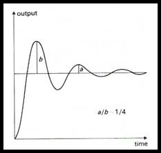
Each time I see these charts, (Fig 2.) I can’t help but be reminded of a control system tuned for quarter decay. See here for an example response:
 ?w=500
and
With the base temperature being around 10 degrees and some cataclysmic event bumps it up to 15 degrees then it oscillates back to 10. Ready for the event to repeat.
Is the second graph correct? Critically and overdamped systems approach their final state asymptotically so do not cross the SP line.
If I have to read a sentence three times, and still have no idea what the author is saying….. ….. I give up!
I highly recommend George Orwell’s ‘Politics and the English Language’ to see what went wrong and goes wrong in so many scientific papers. Sometimes the defect lies in misunderstanding the role of the written word (clear communication), but most often these days it’s because they’re trying to force too much politics into the science … or perhaps the reverse. Other times they’re just trying to baffle you with BS.
Like all of Orwell, it’s a good read with sound advice and insight with an added bonus. After each reading one’s own writing improves.
https://www.orwellfoundation.com/the-orwell-foundation/orwell/essays-and-other-works/politics-and-the-english-language/
And the phrase “judged universally well constrained” & similar is used WAY too often. A dead giveaway.
For me, there were a lot of those sentences.
The basis of paleo Temperature vs. CO2 calcs is the O18 to 016 isotope ratios in foraminifera layers in geologically dated ocean sediment samples. This is very sciency sounding, but shows by proxy that the deep ocean has been as much as 12 C warmer than present at about 50 million years ago. Such a high temperature at that time seems geologically unlikely unless you start from an “I-believe-the-isotope-ratios” viewpoint. And the possibility of the isotope ratio variation being caused by something other than deep ocean temperature is seldom delved into.
Changes over 50 My in ocean salinity, pH, or water soluble trace elements, maybe even background cosmic rays come to mind as items that Temp to Isotope ratio correlation researchers might have assumed to be constant, but maybe aren’t …..Do modern, more sensitive instruments corroborate those curves of the 1970’s ?
1) The figure generally used for Albedo is nonsense. That figure (0.30) is after ‘Climate’ has modified it.
The ‘start’ figure should be that of the Moon, circa 0.12
(Do note here that the Main Green House Gas (water) always and everywhere does everything in its considerable power to cool the Planet Earth)
2) It is not warm under a night-time (or any other time) cloud because of the cloud. The cloud is there as a consequence of a raft of warm air having rolled in from somewhere else. It happens constantly here in the UK, It is called ‘Weather’ and occasioned by anti-cyclonic systems passing over, systems containing cold polar air and warm tropical air
3) The ‘average power’ calculation is garbage. Huge amounts more power arrive at the Equator and Tropics than near the poles and the Equator & Tropics have massively greater area.
Do a proper integration involving sines and cosines, a proper Albedo figure and using a ‘raw’ solar power of 1,372 Watts, the average power landing on the surface of Earth is 370 Watts per square metre
4) It is child-like mathematical naivety to imagine you can average things when one varies as the fourth power of the other.
We know that CO2 was not the primary feedback involved in the modulation of ice ages, because when CO2 concentrations were high the world cooled, and when CO2 was low the world warmed.
That is why I deduced that the primary feedback controlling ice ages, was ice sheet albedo.
Modulation of Ice Ages via Dust and Albedo.
https://www.sciencedirect.com/science/article/pii/S1674987116300305
Ralph
The difference between Ice sheet Albedo and Cloud Albedo being indistinguishable is something worth pondering for you.
I have not factored in atmospheric albedo, because there is a lack of a modulation mechanism that would match the known ice-age cycle.
However, there is a definite and obvious mechanism controlling ice-sheet albedo, and that is dust. Dust is not only inversely proportional to CO2, during all the ice ages, it also peaks just before every interglacial.
Ralph
Ralf, I enjoyed your papers on paleoclimate. I agree that M-cycles are the forcing and ice sheet albedo is the primary amplifying feedback. With those two having predictable forcings has anyone to your knowledge tried to model CO2 feedback forcing through the last 500ka where we have high resolution temperature proxy data? If not what is the variable that prevents the quantification of CO2 forcing there?
We had a disagreement on CO2 feedbacks.
They were saying that the CO2 forcing-feedback was 4 W/m2. But that is over the full 5 ky of an interglacial. The true CO2 forcing is actually 0.008 W/m2 per decade, which is not going to assist anything. And the climate needs to get from one decade to a slightly warmer next decade, with just 0.00’ W/m2. It is not going to happen.
Conversely, dirty ice sheets can provide 240 W/m2 every year, when measures regionally. Now that can and will make a difference .
They said I was crazy.
R
Thanks Ralph. I am going to cite your comment on CE where we are having the same post. I hope you can stop by there too.
And I realized after thinking that they don’t know the forcing for ice sheet albedo if they didn’t factor in the dust effect. Your theory explains the glacial collapse better than any other.
CE? I am not familiar.
.
Climate Etc. or Judith Currydot com
Color me skeptical, but I will reserve judgement until having read the rest.
My skepticism derives from basic equation 1. If I did the math correctly, it yields an ECS of 4.7C. That is far too high. Present ECS can be derived at least three different ways. Callendar’s 1938 curve produces 1.67C. Energy budget models (Lewis and Curry) produce a best estimate of about 1.65C. Bode curve plus observational feedbacks produce 1.7C (a guest post expanding previous comments with reference links was sent to Charles last night).
The reason I reserve judgement is that it is possible that climatic conditions during the time period equation 1 was derived from were sufficiently different that a different ECS pertained. For example, Antarctica was not yet squarely over the south pole.
Not science, just observation: You can be damned sure ECS < 3 when the UN IPCC CliSciFi AR5 had to arbitrarily reduce projected model (average ECS = 3.2) temperatures because the majority of the models were running way too hot.
“Callendar’s 1938 curve produces 1.67C”
Callendar’s 1938 curve held water vapour constant (at 7.5 mm Hg). He never intended it as an estimator of ECS.
Can you show your math please so I can follow to the 4.7 ECS? I saw 1100 ppm and 8 C. The author failed to give the banner statement, the ECS they find.
log(2*A)=log(2)+log(A)
so multiple log(2) by 6.68 and you get Rud’s value.
Thanks.
Willis Eschenbach mentioned in his paper, the idea that climate sensitivity is not a constant, but is dependent itself on temperature (https://wattsupwiththat.com/2021/04/28/a-request-for-real-peer-review/). Maybe one should try to include his observations into this model…
Regards the albedo compliment to feedback, Hansen’s calculations are wrong. He assumed ice-sheet extent as being proportional to sea-level, and thus he smeared the albedo factor out across the entire globe.
This is incorrect, because albedo is a regional feedback. We know this because every ice age began with a northern hemisphere (NH) Great Winter (Milankovitch minimum), and every interglacial began with a NH Great Summer (Milankovitch Maxumum). These temperature changes are NOT initiated by SH Great Summers or Winters.
Thus ice ages are hemispherically asymmetric. Thus it is highly unlikely that the ice age temperature feedback mechanism is CO2, as that is a global gas and would modulate interglacials in either NH or SH Great Summers. And this is not what the data shows.
Likewise, ice albedo feedbacks are regional, not global. Annual winter snow in Canada is melted by insolation (and albedo) on the snow in Canada, not by the temperature in Argentina. And the same is true for Great Winter snows and ice sheets during the ice ages – it is the insolation and albedo of the northern ice sheets that promote interglacial modulation, not a global CO2, and not a misconceived global albedo factor.
This is important, because Hansen’s albedo factor was a lowly globally smeared 4 W/m2. But a regional albedo factor, as measured upon the ice sheets, can be up to 240 W/m2. So what is more likely to melt the vast ice sheets – Hansen’s 4 W/m2 or my 240 W/m2.
Modulation of Ice Ages via Dust and Albedo.
https://www.sciencedirect.com/science/article/pii/S1674987116300305
Ralph
On the sceptics’ side, there is remarkable supposition that the CO2 concentration is predominantly driven by temperature, rather than by human emissions during the industrial age.
This is an unremarkable straw man argument. A minority of skeptics hold that current CO2 increase is temperature driven only. But mostly it is a false characterisation of the skeptical position. Most skeptics – myself included – accept that currently rising CO2 levels are anthropogenic. Recent anthropogenic CO2 is irrelevant to this study owing to the long historic time scales up to hundreds of millions of years.
The paper omits any mention of the robustly and consistently observed lag of several thousand years between temperature and CO2 over the Pleistocene successive glaciations and interglacials, the period covered by the ice core records, with temperature leading CO2. This glaring omission argues against impartiality of this study and instead shows yet another study irresistably motivated to confirm the dogma of CO2 driving temperature. The obvious mechanism for this – solubility of gas in the ocean depending on temperature, is not mentioned, again pointing to huge bias and practically discrediting the study.
Wrote about this. The lag (depending on proxy) is between 800 and 1200 years. This makes sense, since it approximates the estimated deep ocean overturning period.
Thanks Rud!
Which means one cannot develop a consistent theory of the causes of climactic variations based upon land and ocean configurations significantly different from today’s geography. The number of assumptions one must stack up on top of each other leads to madness; nobody can agree on them.
Yeah, that’s why I went from reading mode to scanning mode, my presupposition buffer got full….
A minority of skeptics hold that current CO2 increase is temperature driven only.
It only takes one to be right.
I weigh these empirical relationships more heavily than anything else:
The EPICA CO2 lag is 400-600 years, with a millennial sensitivity of 7.8ppm/°C.
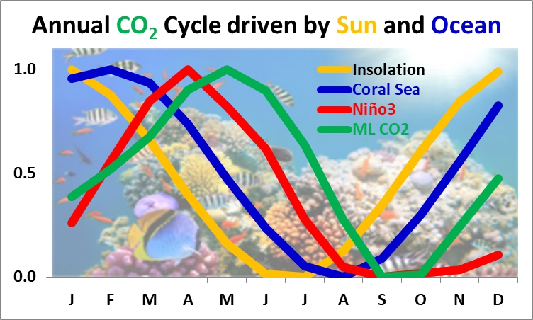
ML CO2 lags ocean temperatures by 10 months with a transient sensitivity of 2.34ppm/°C.
The growth of atmospheric CO2 is a linear function of the temperature and ocean area increase above 25.6°C since the 1850s, not from man-made emissions.
BW, partly agree and partly disagree. The reason is time scales. Plainly there is natural variability as you posit and show, so agree in part. See previous posts here on attribution.
But on short time scales (specifically post 1975) it is easy to prove that most of the Keeling Curve rise in CO2 must be anthropogenic from burning fossil fuels. The proof lies in the changing 12C/13C isotope ratios, as photosynthesis energetically favors the lighter 12C, so more of it is sequestered as fossil fuel, raising relative C13 in the atmosphere. Since both are stable isotopes, if the C13 ratio falls it can only mean 12C rises, and that can only come from burning fossil fuels.
Something is weird there. In the top graph (paleo) you regress ppm CO2 against ΔT. In the bottom graph, you regress (annual Δppm) against ΔT. If you had regressed ppm against ΔT, you would get something over 100, not 2.34.
Appreciate it Rud. The last chapter on CO2 isotopes hasn’t been written.
Thanx Nick I’ll look at it again; if I recall correctly from a few years ago the time period(s) account for this. I was responding to the point about lags, which are correct in both my plots. CO2 changes lag temperature changes without fail, not man-made emissions.
The natural variability is real and misunderstood. Every year ML CO2 follows tropical ocean temperatures like clockwork.
The derivative of Man-Made CO2 emissions follows the derivative of ML CO2 by 2 years, and the ML derivative trend is 5.7X that of MM, meaning MM emissions are not driving the ML CO2 bus:
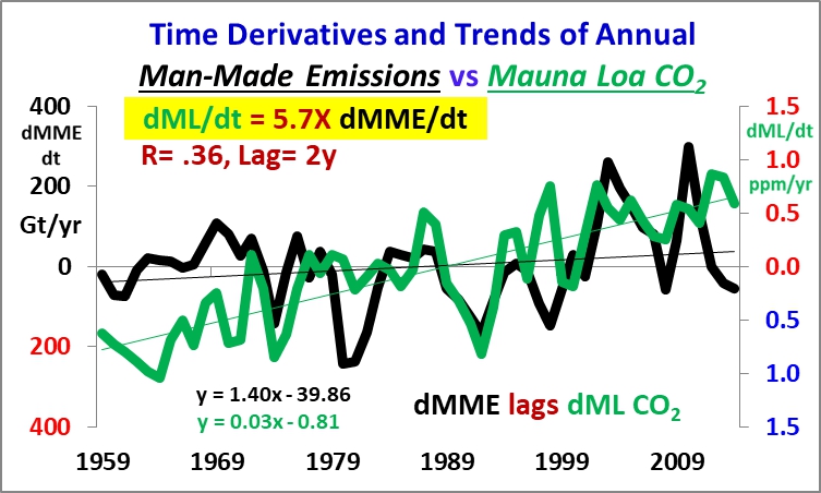
Using departure from average of detrended integrated annual change on both timeseries (MME and ML CO2) reveals the truth- MME don’t drive ML CO2 at all:

These facts are strong evidence that ML CO2 growth is natural.
Science reference books have tables which well document the very substantial variability of the solubility of CO2 in water as the temperature of water changes. Also note the following facts: the temperature of water changes more slowly than the temperature of earth, and the amount of earth covered by water is substantially greater than the amount covered by land. Obvious conclusion – as the temperature of earth changes, it takes a while for the temperature of the oceans to follow, and therefore a lag for the amount of CO2 absorbed by the oceans to follow the change in earth’s temperature. Therefore, the lag in observed change in the amount of CO2 in the atmosphere.
Obvious conclusion – given constant availability of CO2, the amount of CO2 in the atmosphere will follow a change in temperature of earth. CO2 does NOT control earth’s temperature to any substantial degree, it is the other way around!
The amount of CO2 in the atmosphere has increased by about 40% over the past 100 years or so. Earth started warming somewhat prior to the year 1800, BEFORE there was any significant change in CO2 in the atmosphere. Current reports now indicate global cooling while CO2 is still increasing.
“Obvious conclusion – given constant availability of CO2, the amount of CO2 in the atmosphere will follow a change in temperature of earth. CO2 does NOT control earth’s temperature to any substantial degree, it is the other way around!”
That is true, more or less, if you interpret availability as total amount in circulation. But we have greatly increased the availability, by burning CO2. And that will control the temperature.
Burning FF to produce CO2 will have an undetermined positive effect on temperature. The small positive theoretical effect (without positive or negative feedbacks) is less than the uncertainty in our measurements of the vast flows of energy into, within and out of Earth’s climatic system. In no way may one assert that anthropogenic CO2 “will control the temperature.” I’ll need conclusive proof that CO2 is anything but a bit player; UN IPCC CliSciFi modeling games are not proof.
It’s interesting that the author cites Soreghan et al 2019.
These authors get into all sorts of trouble trying to explain the Palaeozoic glaciations from 360-260 Mya. They recognise glaring mis-matches with CO2 and the need to posit low levels of CO2 that would drive plant based life to extinction – and many other inconsistencies also:
The cult of carbon dioxide is leading palaeo-climate research on a road to nowhere – Odyssey (wordpress.com)
In the end they just invoke a string of volcanoes. Volcanoes can only cool climate for a short time – less than a century, so they require a string of volcanoes – millions of them – happening serially. This is hardly plausible except possibly for flood basalt eruptions, of which none occurred during this time.
Particularly acute is the difficulty of attributing the end-Ordovician (Saharan-Andean) glaciation to CO2, in view of the detailed geo-chronology showing that CO2 levels increased during the inception of this profound glaciation and remained high throughout it:
The Ordovician glaciation – glaciers spread while CO2 increased in the atmosphere: a problem for carbon alarmism – Odyssey (wordpress.com)
If Anderl wishes to adequately model the strong influence of tectonic shift and continental configuration on climate and temperature, the factors to focus on would include:
– Total land area
– Amount of land around the equator
– Amount of land at the poles
– Collisions and separations
– Mountain uplift from collisions e.g. Himalayas from India collision
– A meridionally bounded ocean i.e. the Atlantic
– Area of shallow seas
The current fashion to ignore all aspects of continental movement except for silicate weathering (since it influences CO2) is not helpful.
To tectonic factors I should add:
This paper clearly shows that CO2 and temperature are related and that relationship is very strong. However, what it ignores is causation. It assumes since they are related then one must cause the other. It is not only likely, but most probable that both are driven by other related factors. For example during periods of high volcanism both large amounts of CO2 and ash are injected into the atmosphere. CO2 would go up and temp would go down. As the ash cleared, the temp would go up and the CO2 would slowly disapate. The overall effect would depend on the global level of this activity and the period of time involved. It is clear from the recent geologic past that there is yet much to be learned and it is way to early to say it is settled science. Just the ocean chemistry alone is mind numbing.
No it just shows they are playing the tuning game
Younger dryas, predicted? Big asteroid that killed off dinosaurs predicted? Three/four glaciation predicted?
Color me just a bit skeptical. Something tells me just a few tuned parameters are be played with.
“However during the current geologic eon, the water content in the atmosphere is a passive reactant to otherwise driven temperatures, acting as an amplifier. “
Ummm, what? Did water content just stop doing what it’s always been doing??
“the water content in the atmosphere is a passive reactant to otherwise driven temperatures, acting as an amplifier. “
Or maybe water content acts as a damper instead. Moeller estimated that a two percent increase in cloud cover (which reflects more sunlight) would offset all of the temperature increase caused by human-derived CO2.
I see lots of hand waving.
Thomas, I can only conclude that with such a high model climate sensitivity you are simply modeling a spurious correlation of outgassing CO2 CAUSED by rising temperatures, and not the other way round.
I skimmed the paper and thought huh? That must yield an ECS of close to 5 deg C! So Rud saved me the trouble and did the math… 4.7 C. If ECS was 4.7 C there would be NO debate about CO2’s effects, they would be LEAPING out of the temperature data screaming look at me! look at me! They’re not. Probably why they didn’t spell out the results of their calculations it instantly calls the results into question.
The real hint that the fix was in though is the straw man not so cleverly hidden in the text. The begin with “skeptics say X” and proceed with an argument that I suppose some skeptics do in fact make, but its not exactly pervasive or even central to the skeptic viewpoint. So they start by putting words into skeptic’s mouths and finish by concluding they are wrong while quietly burying out of site that their own math yields a sensitivity calculation that is absurd.
Here is something on how salinity can affect ocean deep water formation to be either a warming or cooling influence on global climate, and could explain globally equable climates of the past.
https://core.ac.uk/download/pdf/33671934.pdf
In my case some of that “scepticism” arose about 15 or 20 years ago when I looked at the detail of the falling curve from the Eemian interglacial using the Vostok data.
The attached image is an updated version with EPICA Dome-C data added.
After checking for yourself I hope you will agree there is nothing “remarkable” about that particular “supposition” (only questions about the justification for adding the “predominantly” qualifier without clarifying what timescale[s] you’re talking about).
Notes
The time resolution for the CO2 data (from gas bubbles, subject to diffusion during formation …) is much lower than for temperature (“directly” from deuterium ratios in the ice in each slice of the ice-cores).
EPICA actually re-used the Vostok CO2 data from 22 to 393 kya.
They only extracted and analysed new “gas bubble” contents from 22kya to “0” (Monnin et al, 2001, with finer time resolution) and from 800 to 393 kya (Lüthi et al, 2008 and Siegenthaler et al, 2005).
Vostok (D-ratio temps –> GMST) scaling = 0.5 (as used in the ATL article).
EPICA scaling = 0.44 (to match the “glacial-min to interglacial-peak” delta of ~6°C).
From 128 to 133kya CO2 levels bounced around between 260 and 280ppm (right-hand axis).
Temperatures did a “fall from peak + a long, slow dead-cat bounce” instead.
NB : The “break to the downside” for CO2 occurred around 112 or 113kya, when (global mean) temperatures had already fallen by around 2.5°C (Vostok) or 3°C (EPICA) from the “Anomaly = +0.5°C” level common to both ice-cores between 124 and 127kya.
Vostok and EPICA temperatures diverge between 107 and 98kya, and there is an apparent “phase shift” from roughly 95kya (?) to the end-date shown (they realign for the Holocene glacial-to-interglacial transition around 20-12kya).
I’m guessing this is covered in other scientific papers I am (currently) unaware of.
Just looking at the graph, many of the “rebounds” (especially around 87-83kya and 78-72kya) clearly show CO2 lagging temperature, whichever “phase shift” (/ age model) is used.
CO2 levels in the attached graph never go above the 285-290ppm range.
The additional effects from CO2 levels above 300 (or 350, or 400, or …) ppm, especially their timing / delay parameters, are very much TBD.
This kind of excellent comment is why I come to WUWT.
I’m including you in there, too, Rud. 🙂
From the article: “Regarding the atmospheric composition, CO2 is recognized as a temperature driving agent.”
Yes, but the question is: which way does it drive temperature? Up or down? A second question is: By how much?
Additonal CO2 in the atmosphere may result in net atmospheric cooling (Moeller).
The “CO2 Science” is not settled.
The Inconvienient facts:
https://imgur.com/q4RTtDw
I will just comment in simple street-talk English.
There really is little need to resort to using paleoclimatology proxies, or much real benefit to be gained by debating whether lower atmospheric temperature drives atmospheric CO2 concentration or CO2 atmospheric concentration drives lower atmospheric temperature when considering the following.
Nature and the progress of time test climate models for us.
So far, as concerns CO2 driving global lower atmosphere temperature (GLAT), there is a null result.
Simply put, Earth has experienced two significant periods of nearly-constant GLAT (approximately, from 1940-1975 and from 1997-present) based on accurate scientific measurements; this DESPITE global atmospheric CO2 levels having a smooth, continuously-increasing exponential trend, also accurately measured, over these same time periods . . . and there being a very significant 35% total CO2 ppm increase from 1940 to present.
Note that both NASA and NOAA define “climate” as being weather averaged over a specified geographic area for a period of 30 years or more. The span of 1940-1975 meets this criteria; the timespan from 1997 to present is just 6 years short of this.
But also note much more CO2 (on a volume basis) has been put into the atmosphere in this latter time span than was put into the atmosphere during the span of 1940-1975.
As Nobel prize-winning physicist Richard Feynman is famously quoted as saying, ““It doesn’t matter how beautiful your theory is, it doesn’t matter how smart you are. If it doesn’t agree with experiment, if it doesn’t agree with observation, it’s wrong. That’s all there is to it.”
I appreciate the time and effort expended to create and report on Part 1 of “Simplified climate modelling”, and I expect to have similar appreciation for subsequent parts of what is sure to be a magnum opus by Mr. Anderl. Adding to human understanding is always important. However, I also believe there are short paths to traverse a given forest.
A lot of words strung together telling us very little