By Christopher Monckton of Brenchley
This is a long and technical posting. If you don’t want to read it, don’t whine.
The first scientist to attempt to predict eventual warming by doubled CO2, known to the crystal-ball gazers as equilibrium doubled-CO2 sensitivity (ECS), was the Nobel laureate Svante Arrhenius, a chemist, in 1896. He had recently lost his beloved wife. To keep his mind occupied during the long Nordic winter, he carried out some 10,000 spectral-line calculations by hand and concluded that ECS was about 5 C°.
However, he had relied upon what turned out to be defective lunar spectral data. Realizing this, he recalculated ten years later and, in 1906, published a second paper, in which he did what climate “scientists” refuse to do today: he recanted his first paper and published a revised estimate, this time in German, which true-believing Thermageddonites seldom cite:

His corrected calculation, published in the then newly-founded Journal of the Royal Nobel Institute, suggested 1.6 C° ECS, including the water-vapor feedback response.
Guy Stewart Callendar, a British steam engineer, published his own calculation in 1938, and presented his result before the Royal Society (the Society’s subsequent discussion is well worth reading). He, too, predicted 1.6 C° ECS, as the dotted lines I have added to his graph demonstrate:

Then there was a sudden jump in predicted ECS. Plass (1956) predicted 3.6 C° ECS. Möller (1963) predicted a direct or reference doubled-CO2 sensitivity (RCS) of 1.5 C°, rising to as much as 9.6 C° if relative humidity did not change. He added an important rider: “…the variation in the radiation budget from a changed CO2 concentration can be compensated for completely without any variation in the surface temperature when the cloudiness is increased by +0.006.” Unsurprisingly, he concluded that “the theory that climatic variations are effected by variations in the CO2 content becomes very questionable.”
Manabe & Wetherald (1975), using an early radiative-convective model, predicted 2.3 C° ECS. Hansen (1981) gave a midrange estimate of 2.8 C° ECS. In 1984 he returned to the subject, and, for the first time, introduced feedback formulism from control theory, the study of feedback processes in dynamical systems (systems that change their state over time). He predicted 1.2 C° RCS and 4 C° ECS, implying a feedback fraction 0.7.
In 1988, in now-notorious testimony before the U.S. Senate during a June so hot that nothing like it has been experienced in Washington DC since, he predicted 3.2 C° per century (broadly equivalent to ECS) on a business-as-usual scenario (and it is the business-as-usual scenario that has happened since), but anthropogenic warming is little more than a third of his predicted business-as-usual rate:

In 1988 the late Michael Schlesinger returned to the subject of temperature feedback, and found that in a typical general-circulation model the feedback fraction – i.e., the fraction of equilibrium sensitivity contributed by feedback response – was an absurdly elevated 0.71, implying a system-gain factor (the ratio of equilibrium sensitivity after feedback to reference sensitivity before it) of 3.5 and thus, assuming 1.05 RCS, an ECS of 3.6 C°.
Gregory et al. (2002) introduced a simplified method of deriving ECS using an energy-balance method. Energy-balance methods had been around for some time, but it was not until the early 2000s that satellite and ocean data became reliable enough and comprehensive enough to use this simple method. Gregory generated a probability distribution, strongly right-skewed (for a reason that will become apparent later), with a midrange estimate of 2 C° ECS:

Gregory’s result has been followed by many subsequent papers using the energy-balance method. Most of them find ECS to be 1.5-2 C°, one-third to one-half of the 3.7-4 C° midrange that the current general-circulation models predict.
In 2010 Lacis et al., adhering to the GCMs’ method, wrote:
“For the doubled-CO2 irradiance forcing, … for which the direct no-feedback response of the global surface temperature [is] 1.2 C° …, the ~4 C° surface warming implies [a] … [system-gain factor] of 3.3. … “
Lacis et al. went on to explain why they thought there would be so large a system-gain factor, which implies a feedback fraction of 0.7:
Noncondensing greenhouse gases, which account for 25% of the total terrestrial greenhouse effect, … provide the stable temperature structure that sustains the current levels of atmospheric water vapor and clouds via feedback processes that account for the remaining 75% of the greenhouse effect.
Unfortunately, the above passage explicitly perpetrates an extraordinary error, universal throughout climatology, which is the reason why modelers expect – and hence their models predict – far larger warming than the direct and simple energy-balance method would suggest. The simple block diagram below will demonstrate the error by comparing erroneous (red) against corrected (green) values all round the loop:

Let us walk round the feedback loop for the preindustrial era. We examine the preindustrial era because when modelers were first trying to estimate the influence of the water-vapor and other feedbacks, none of which can be directly and reliably quantified by measurement or observation, they began with the preindustrial era.
For instance, Hansen (1984) says:
“… this requirement of energy balance yields [emission temperature] of about 255 K. … the surface temperature is about 288 K, 33 K warmer than emission temperature. … The equilibrium global mean warming of the surface air is about 4 C° … This corresponds to a [system-gain factor] 3-4, since the no-feedback temperature change required to restore radiative equilibrium with space is 1.2-1.3 C°.
First, let us loop the loop climatology’s way. The direct warming by preindustrial noncondensing greenhouse gases (the condensing gas water vapor is treated as a feedback) is about 8 K, but the total natural greenhouse effect, the difference between the 255 K emission temperature and the 287 K equilibrium global mean surface temperature in 1850 is 32 K. Therefore, climatology’s system-gain factor is 32 / 8, or 4, so that its imagined feedback fraction is 1 – 1/4, or 0.75 – again absurdly high. Thus, 1 K RCS would become 4 K ECS.
Now let us loop the loop control theory’s way, first proven by Black (1934) at Bell Labs in New York, and long and conclusively verified in practice. One must not only input the preindustrial reference sensitivity to noncondensing greenhouse gases into the loop via the summative input/output node at the apex of the loop: one must also input the 255 K emission temperature (yellow), which is known as the input signal (the clue is in the name).
It’s the Sun, stupid!
Then the output from the loop is no longer merely the 32 K natural greenhouse effect: it is the 287 K equilibrium global mean surface temperature in 1850. The system-gain factor is then 287 / (255 + 8), or 1.09, less than a third of climatology’s estimate. The feedback fraction is 1 – 1 / 1.09, or 0.08, less by an order of magnitude than climatology’s estimate.
Therefore, contrary to what Hansen, Schlesinger, Lacis and many others imagine, there is no good reason in the preindustrial data to expect that feedback on Earth is unique in the solar system for its magnitude, or that ECS will be anything like the imagined three or four times RCS.
As can be seen from the quotation from Lacis et al., climatology in fact assumes that the system-gain factor in the industrial era will be about the same as that for the preindustrial era. Therefore, the usual argument against the corrected preindustrial calculation – that it does not allow for inconstancy of the unit feedback response with temperature – is not relevant.
Furthermore, a simple energy-balance calculation of ECS using current mainstream industrial-era data in a method entirely distinct from the preindustrial analysis and not dependent upon it in any way comes to the same answer as the corrected preindustrial method: a negligible contribution from feedback response. Accordingly, unit feedback response is approximately constant with temperature, and ECS is little more than the 1.05 K RCS.
Why, then, do the models get their predictions so wrong? In the medium term (top of the diagram below), midrange projected anthropogenic medium-term warming per century equivalent was 3.4 K as predicted by IPCC in 1990, but observed warming was only 1.65 K, of which only 70% (Wu et al. 2019), or 1.15 K, was anthropogenic. IPCC’s prediction was thus about thrice subsequently-observation, in line with the error but not with reality.

Since the currently-estimated doubled-CO2 radiative forcing is about the same as predicted radiative forcing from all anthropogenic sources over the 21st century, one can observe in the latest generation of models much the same threefold exaggeration compared with the 1.1 K ECS derivable from current climate data (bottom half of the above diagram), including real-world warming and radiative imbalance, via the energy-balance method.
The error of neglecting the large feedback response to emission temperature, and of thus effectively adding it to, and miscounting it as though it were part of, the actually minuscule feedback response to direct greenhouse-gas warming, is elementary and grave. Yet it seems to be universal throughout climatology. Here are just a few statements of it:
The American Meteorological Society (AMS, 2000) uses a definition of feedback that likewise overlooks feedback response to the initial state –
“A sequence of interactions that determines the response of a system to an initial perturbation”.
Soden & Held (2006) also talk of feedbacks responding solely to perturbations, but not also to emission temperature–
“Climate models exhibit a large range of sensitivities in response to increased greenhouse gases due to differences in feedback processes that amplify or dampen the initial radiative perturbation.”
Sir John Houghton (2006), then chairman of IPCC’s climate-science working party, was asked why IPCC expected a large anthropogenic warming. Sir John replied that, since preindustrial feedback response accounted for three-quarters of the natural greenhouse effect, so that the preindustrial system-gain factor was , and one would thus expect a system-gain factor of
or
today.
IPCC (2007, ch. 6.1, p. 354) again overlooks the large feedback response to the 255 K emission temperature:
“For different types of perturbations, the relative magnitudes of the feedbacks can vary substantially.”
Roe (2009), like Schlesinger (1988), shows a feedback block diagram with a perturbation ∆R as the only input, and no contribution to feedback response by emission temperature –

Yoshimori et al. (2009) say:
“The conceptually simplest definition of climate feedback is the processes that result from surface temperature changes, and that result in net radiation changes at the top of the atmosphere (TOA) and consequent surface temperature changes.”
Lacis et al. (2010) repeat the error and explicitly quantify its effect, defining temperature feedback as responding only to changes in the concentration of the preindustrial noncondensing greenhouse gases, but not also to emission temperature itself, consequently imagining that ECS will be times the
degree direct warming by those gases:
“This allows an empirical determination of the climate feedback factor [the system-gain factor] as the ratio of the total global flux changeto the flux change that is attributable to the radiative forcing due to the noncondensing greenhouse gases. This empirical determination … implies that Earth’s climate system operates with strong positive feedback that arises from the forcing-induced changes of the condensable species. … noncondensing greenhouse gases constitute the key 25% of the radiative forcing that supports and sustains the entire terrestrial greenhouse effect, the remaining 75% coming as fast feedback contributions from the water vapor and clouds.”
Schmidt et al. (2010) find the equilibrium doubled-CO2 radiative forcing to be five times the direct forcing:
“At the doubled-CO2 equilibrium, the global mean increase in … the total greenhouse effect is ~20 W m-2, significantly larger than the ≥ 3initial forcing and demonstrating the overall effect of the long-wave feedbacks is positive (in this model).”
IPCC (2013, p. 1450) defines what Bates (2016) calls “sensitivity-altering feedback” as responding solely to perturbations, which are mentioned five times, but not also to the input signal, emission temperature:
“Climate feedback: An interaction in which a perturbation in one climate quantity causes a change in a second, and the change in the second quantity ultimately leads to an additional change in the first. A negative feedback is one in which the initial perturbation is weakened by the changes it causes; a positive feedback is one in which the initial perturbation is enhanced … the climate quantity that is perturbed is the global mean surface temperature, which in turn causes changes in the global radiation budget. … the initial perturbation can … be externally forced or arise as part of internal variability.”
Knutti & Rugenstein (2015) likewise make no mention of base feedback response:
“The degree of imbalance at some time following a perturbation can be ascribed to the temperature response itself and changes induced by the temperature response, called feedbacks.”
Dufresne & St.-Lu (2015) say:
“The response of the various climatic processes to climate change can amplify (positive feedback) or damp (negative feedback) the initial temperature perturbation.”
Heinze et al. (2019) say:
“The climate system reacts to changes in forcing through a response. This response can be amplified or damped through positive or negative feedbacks.”
Sherwood et al. 2020 also neglect emission temperature as the primary driver of feedback response –
“The responses of these [climate system] constituents to warming are termed feedback. The constituents, including atmospheric temperature, water vapor, clouds, and surface ice and snow, are controlled by processes such as radiation, turbulence, condensation, and others. The CO2 radiative forcing and climate feedback may also depend on chemical and biological processes.”
The effect of the error is drastic indeed. The system-gain factor and thus ECS is overstated threefold to fourfold; the feedback fraction is overestimated tenfold; and the unit feedback response (i.e., the feedback response per degree of direct warming before accounting for feedback) is overstated 30-fold at midrange and 100-fold at the upper bound of the models’ predictions.
The error can be very simply understood by looking at how climatology and control theory would calculate the system-gain factor based on preindustrial data:

Since RCS is little more than 1 K, ECS once the sunshine temperature of 255 K has been added to climatology’s numerator and denominator to calm things down, is little more than the system-gain factor. And that is the end of the “climate emergency”. It was all a mistake.
Of course, the models do not incorporate feedback formulism directly. Feedbacks are diagnosed ex post facto from their outputs. Recently an eminent skeptical climatologist, looking at our result, said we ought to have realized from the discrepancy between the models’ estimates of ECS and our own that we must be wrong, because the models were a perfect representation of the climate.
It is certainly proving no less difficult to explain the control-theory error to skeptics than it is to the totalitarian faction that profiteers so mightily by the error. Here, then, is how our distinguished co-author, a leading professor of control theory, puts it:
Natural quantities are what they are. To define a quantity as the sum of a base signal and its perturbation is a model created by the observer. If the base signal – analogous to the input signal in an electronic circuit – is chosen arbitrarily, the perturbation (the difference between the arbitrarily-chosen baseline and the quantity that is the sum of the baseline and the perturbation) ceases to be a real, physical quantity: it is merely an artefact of a construct that randomly divides a physical quantity into multiple components. However, the real system does not care about the models created by its observer. This can easily be demonstrated by the most important feedback loop of all, the water vapour feedback, where warming causes water to evaporate and the resulting water vapour, a greenhouse gas, forces additional warming.
Climatology defines feedback in such a way that only the perturbation – but not also the base signal, emission temperature – triggers feedback response. The implication is that in climatologists’ view of the climate the sunshine does not evaporate any water. In their models, the 1363.5 W m-2 total solar irradiance does not evaporate a single molecule of water, while the warming caused by just 25 W m-2 of preindustrial forcing by noncondensing greenhouse gases is solely responsible for all the naturally-occurring evaporation of water on earth. This is obvious nonsense. Water cares neither about the source of the heat that evaporates it nor about climatology’s erroneous definitions of feedback. In climatology’s model, the water vapour feedback would cease to work if all the greenhouse gases were removed from the atmosphere. The Sun, through emission temperature, would not evaporate a single molecule of water, because by climatologists’ definition sunshine does not evaporate water.
Heat is the same physical quantity, no matter what the source of the heat is. The state of a system can be described by the heat energy it contains, no matter what the source of the heat is. Temperature-induced feedbacks are triggered by various sources of heat. The Sun is the largest such source. Heat originating from solar irradiance follows precisely the same natural laws as heat originating from the greenhouse effect does. All that counts in analysing the behaviour of a physical system is the total heat content, not its original source or sources.
Climatology’s models fail to reflect this fact. A model of a natural system must reflect that system’s inner workings, which may not be defined away by any “consensus”. The benchmark for a good model of a real system is not “consensus” but objective reality. The operation of a feedback amplifier in a dynamical system such as the climate (a dynamical system being one that changes its state over time) is long proven theoretically and repeatedly demonstrated in real-world applications, such as control systems for power stations, space shuttles, the flies on the scape-shafts of church-tower clocks, the governors on steam engines, and increased specific humidity with warmer weather in the climate, and the systems that got us to the Moon.
Every control theorist to whom we have shown our results has gotten the point at once. Every climatologist – skeptical as well as Thermageddonite – has wriggled uncomfortably. For control theory is right outside climatology’s skill-set and comfort zone.
So let us end with an examination of why it is that the “perfect” models are in reality, and formally, altogether incapable of telling us anything useful whatsoever about how much global warming our industries and enterprises may cause.
The models attempt to solve the Navier-Stokes equations using computational fluid dynamics for cells typically 100 km x 100 km x 1 km, in a series of time-steps. Given the surface area of of the Earth and the depth of the troposphere, the equations must be solved over and over again, time-step after time-step, for each of about half a million such cells – in each of which many of the relevant processes, such as Svensmark nucleation, take place at sub-grid scale and are not captured by the models at all.
Now the Navier-Stokes equations are notoriously refractory partial differential equations: so intractable, in fact, that no solutions in closed form have yet been found. They can only be solved numerically and, precisely because no closed-form solutions are available, one cannot be sure that the numerical solutions do not contain errors.
Here are the Navier-Stokes equations:

So troublesome are these equations, and so useful would it be if they could be made more tractable, that the Clay Mathematics Institute is offering a $1 million Millennium Prize to the first person to demonstrate the existence and smoothness (i.e., continuity) of real Navier-Stokes solutions in three dimensions.
There is a further grave difficulty with models that proceed in a series of time-steps. As Pat Frank first pointed out in a landmark paper of great ingenuity and perception two years ago – a paper, incidentally, that has not yet met with any peer-reviewed refutation – propagation of uncertainty through the models’ time-steps renders them formally incapable of telling us anything whatsoever about how much or how little global warming we may cause. Whatever other uses the models may have, their global-warming predictions are mere guesswork, and are wholly valueless.
One problem is that the uncertainties in key variables are so much larger than the tiny mean anthropogenic signal of less than 0.04 Watts per square meter per year. For instance, the low-cloud fraction is subject to an annual uncertainty of 4 Watts per square meter (derived by averaging over 20 years). Since propagation of uncertainty proceeds in quadrature, this one uncertainty propagates so as to establish on its own an uncertainty envelope of ±15 to ±20 C° over a century. And there are many, many such uncertainties.
Therefore, any centennial-scale prediction falling within that envelope of uncertainty is nothing more than a guess plucked out of the air. Here is what the uncertainty propagation of this one variable in just one model looks like. The entire interval of CMIP6 ECS projections falls well within the uncertainty envelope and, therefore, tells us nothing – nothing whatsoever – about how much warming we may cause.

Pat has had the same difficulty as we have had in convincing skeptics and Thermageddonites alike that he is correct. When I first saw him give a first-class talk on this subject, at the World Federation of Scientists’ meeting at Erice in Sicily in 2016, he was howled down by scientists on both sides in a scandalously malevolent and ignorant manner reminiscent of the gross mistreatment of Henrik Svensmark by the profiteering brutes at the once-distinguished Royal Society some years ago.
Here are just some of the nonsensical responses Pat Frank has had to deal with over the past couple of years since publication, and before that from reviewers at several journals that were simply not willing to publish so ground-breaking a result:
Nearly all the reviewers of Dr Frank’s paper a) did not know the distinction between accuracy and precision; b) did not understand that a temperature uncertainty is not a physical temperature interval; c) did not realize that deriving an uncertainty to condition a projected temperature does not imply that the model itself oscillates between icehouse and greenhouse climate predictions [an actual objection from a reviewer]; d) treated propagation of uncertainty, a standard statistical method, as an alien concept; e) did not understand the purpose or significance of a calibration experiment; f) did not understand the concept of instrumental or model resolution or their empirical limits; g) did not understand physical uncertainty analysis at all; h) did not even appreciate that ±n is not the same as +n; i) did not realize that the ± 4 W m–2 uncertainty in cloud forcing was an annual mean derived from 20 years’ data; j) did not understand the difference between base-state error, spatial root-mean-square error and global mean net error; k) did not realize that taking the mean of uncertainties cancels the signs of the errors, concealing the true extent of the uncertainty; l) did not appreciate that climate modellers’ habit of taking differences against a base state does not subtract away the uncertainty; m) imagined that a simulation error in tropospheric heat content would not produce a mistaken air temperature; did not understand that the low-cloud-fraction uncertainty on which the analysis was based was not a base-state uncertainty, nor a constant error, nor a time-invariant error; n) imagined that the allegedly correct 1988-2020 temperature projection by Hansen (1988) invalidated the analysis.
Bah! We have had to endure the same sort of nonsense, and for the same reason: climatologists are insufficiently familiar with relevant fields of mathematics, physics and economics outside their own narrow and too often sullenly narrow-minded specialism, and are most unwilling to learn.
The bottom line is that climatology is simply wrong about the magnitude of future global warming. No government should pay the slightest attention to anything it says.
Discover more from Watts Up With That?
Subscribe to get the latest posts sent to your email.
I THINK I understand this for the first time! Thank you, Christopher.
“The Sun is the largest such source.”
Surely the sun is the only heat source.
As I understand it over land, radiative gases keep the terrestrial IR from solar input close to the ground (where actual summer dry surface temperatures easily reach 55ºC) to create instability for convection to cool the surface and warm the boundary layer with sensible heat and add latent heat above it up to the tropopause.
At night, radiation mainly from the boundary layer that was warmed by that daytime convection resists radiative cooling of the surface. Cooling by CO2 occurs above the tropopause.
Overall more solar energy has been converted into sensible and latent heat than would otherwise have been be the case, but atmospheric dynamics moves that extra energy from the tropic to the poles, cooling the former and warming the latter.
Earth itself is also a source of heat, both latent from its creation and due to radioactive decay. At its present age, those two causes produce about equal amounts of heat.
Practically true.
But there is another nuclear reactor inside the Earth that keeps spewing out heat though volcanoes.
David Douglass did an interesting paper some years ago showing that the warmth from the Earth’s interior was not negligible and should be explicitly taken into account.
There are other sources than the sun. There are sub-surface sources like volcanoes. And there are releases from stored solar energy (plants, etc.) that are excess heat from their use (combustion, etc.). The calculations typically refer to the sun as a source only for immediate heat not stored. I maintain that the sun is ultimately almost the only source as sub-surface contributions are relatively minimal.
A minor point.. on your block diagram you have written “non-consensing GHG’s”..
Many thanks for spotting this one. Perhaps I should have written “non-consenting GHGs”.
Fantastic! I love the lord.
I also figured out long ago that warming by (more) CO2 must lead to a higher minimum temperature. Guess my surprise: nobody wants to look at minima!
My own results back in 2015 showed that minima were dropping:
https://documentcloud.adobe.com/link/track?uri=urn:aaid:scds:US:1ca524a0-7733-4918-ba6d-e0b37f01a553
Read my graph from right to left. In 2015, minima were dropping by 0.01K /annum. Over the past 20 years minima must have dropped by ca. 0.2K.
(the sample of weather stations was balanced on latitude and 70/30 @sea/inland
Looks like I was right…after all. As usual, it feels a bit like pissing in your own (black) pants: it gives a warm feeling, but nobody notices it.
Tony also exposes NASA data tampering which hides the minima … https://newtube.app/TonyHeller/hpBtSRL
I also picked up tempering with minima by MET. The results in Gibraltar don’ t tie up with the data of surrounding stations in Spain and Marocco.
Henry,
My analysis indicates that there is a sinusoidal variation in the long-term changes, with a general upwards trend; they are approximately in phase with a period of about 70 years. However, there has recently been a change in the trend of the difference in the two temp’s, starting about 1983. It appears that the increase in the highs was outpacing the lows, possibly a contamination resulting from UHI
https://wattsupwiththat.com/2015/08/11/an-analysis-of-best-data-for-the-question-is-earth-warming-or-cooling/
The sinus is there. You are seeing about half of it in my picture. Sorry. I dont trust any of the official data sets.
Why dont they look at minima, anyway.
I strongly agree with the article. This is not the first time this has been discussed on WUWT. Monckton has made a similar point.
The problem is that climate science and control theory use the word “Feedback” differently and they should have different names.
Feedback in climate science is the first derivative of Feedback in control theory.
Feedback in control theory is the integral of Feedback in climate science.
Think of the steering wheel on a car. When you turn, negative feedback tries to resist the turn and return you to a straight line. Control theory says that the feedback is proportional to how far you turn away from a straight line.
Climate science on the other hand says that feedback is proportional to a change in the position of the steering wheel, regardless of starting value. So a turn of 1 inch to the right will generate the exact same feedback, regardless of whether you are going straight or already in a hard turn to the right.
Control theory says the climate science approach is in error, and would only generate the correct answer in very special cases, confined to cars that are either parked or with very dangerous steering. The sort of car that could be expected to drive you into a ditch if you turned the wheel past the “tipping point”/
This illustration is very clear.
Thank you.
Well stated. This was why I kept getting confused with feedback discussions. Glad you made these distinctions.
You forgot the scenario with positive feedback where when you turn an inch the car actually turns 2 inches which then goes to 4 more inches. Maybe that is your tipping point?
Runaway positive feedback.
My admiration to Christopher for his extraordinary work, and my deep appreciation to him for discussing my own.
I also greatly appreciate Christopher’s tenacious treatment of the feedback issue as updated and re-stated here. And yes, it was great to see your work (Pat Frank) credited and characterized appropriately.
Many thanks to Pat Frank and to David Dibbell for their kind remarks. Pat Frank’s paper is of enormous importance: it demonstrates formally that, whatever value models may have in other directions, models’ predictions of global temperature change are no better than guesswork.
Now the Navier-Stokes …, one cannot be sure that the numerical solutions do not contain errors..
==========
You can be guaranteed they contain errors, even if they calculate the value correctly, simply due to “loss of precision” and similar errors that build up at each iteration. As a result grid cells will leak or gain energy over time, making the long term forecast unreliable.
These errors are not subject to the law of large numbers, climate politicians to the contrary. Otherwise you could use “pin the tail on the donkey” as a model to forecast the future. Increase the number of players, and you will get more tails on the donkey, then take the “ensemble mean” (IPCC).
I learned this in a graduate class in the late 1980’s on parallel computing. The weather/climate models were a great example for “we still need a bigger/better computer” that had to be tempered with the understanding of numerical computing errors. Unfortunately climate model makers know this is still true, but the climate propagandists claim the models are a success today by either ignoring the latter or proclaiming the former has been solved. I’m guessing all the conscientious climate model makers left the business long ago as they couldn’t stand their work being so evilly misrepresented.
Read the book from Mototaka Nakamura, “Confessions of a Climate Scientist”. It is available on Kindle for free.
Right you are, as Dr. Christopher Essex so thoroughly explained.
Digital computers are fundamentally incapable of representing the real world, because all digital computers are inherently deterministic, which the real world is not. The real world is made of quanta which interact with some degree of non-determinism. It isn’t just the inherent ability to measure, it’s also the fact that the act of measurement influences the result. This cannot happen, or even be approximated, in a deterministic system like a digital computer.
I have often wondered if AI is inherently limited because of this. The idea that there could be a sentient digital computer looks to me like science fiction just on this basis.
-BillR
Not sure I entirely agree with BillR. At the quantum level, we cannot make accurate predictions and have to rely upon probabilities because the behavior of particles is chaotic. But chaotic is not the same thing as random. A chaotic system – such as the climate – is not random: it is deterministic but indeterminable in the absence of perfect information, particularly about the initial conditions.
I once co-authored a paper with the late Fred Singer on this subject, but the editor of the journal refused to publish it if I were named as a co-author (even though it was I who had supplied the chaos-theory analysis in the paper). So it was published under Fred’s name alone. The intolerance of the far-Left climate-change establishment is endearingly pathetic.
Well, it certainly makes for an interesting discussion.
Chaos involves self-interaction with (as I recall) a minimum of three paths; this may or may not look like random behavior. A truly random process exhibits Normal probability distribution. The universal example of random behavior in nature is radioactive decay of a single atom.
I am not aware of any process that can affect radioactive decay rates that does not also involve nuclear reactions such as electron capture, muon capture, nuclear fission, or transmutation. I don’t think these processes are chaotic, but perhaps in some way they are.
-BillR
According to Dr Happer Greta is the great granddaughter of Svante Arrhenius, imagine!
Greta isn’t descended from Arrhenius. Her dad is named for him, as a distant relative.
“How Climate Science Gets Distorted”5/5/2021
“Alex Epstein interviews economist Ross McKittrick, famous for debunking Michael Mann’s once-ubiquitous “hockey stick,” about how climate science gets distorted–so that what the public hears about climate science is a wild exaggeration of what most climate scientists actually believe. McKittrick explains: – How the “hockey stick” became ubiquitous despite widespread concerns about its (in)validity. – The real track record of climate models. – Why climate economists are coming under attack for rejecting climate catastrophism. – Why climate catastrophists face a reckoning over the next 10 years. – What we can expect from the UN IPCC’s upcoming AR 6. – Why we almost never discuss the benefits of fossil fuels, including their role in driving progress.”
Soon everything will be cleared up and the global warming spook will be over once and for all. Interesting times ahead. Till then however, I suggest to play a little bit with modtran, as it brings up quite significant insights.
http://climatemodels.uchicago.edu/modtran/modtran.html
With the default setting for a tropical atmosphere emissions are 298.52W/m2 with a surface temperature of 299.7K
If we double CO2 emissions will sink to 295.151W/m2. To hold emissions constant, we will have add a temperature offset. Holding vapor constant an offset of 0.76K is enough to be back at 298.52W/m2.
If we hold relative humidity constant, the offset will need to be larger as a vapor feedback will be included. Now, with plus 1.21K we are back to 298.52W/m2 in emissions. That is an ECS of only 1.21K.
Something weird happens however if we add clouds to the model. Not that we have all too realistic options here, but it should work to outline the problem. Again, we go back to default values. Now we add “Altostratus Cloud … Top 3.0km”. Reality differs in the way that clouds reach up much higher (especially in the tropics), multiplying their impact, while of course we do not have a monolithic constant cloud cover. Overall this scenario still understates the actual impact of clouds. Anyhow..
With this scenario we have 269.004W/m2 in emissions at 400ppm. If we double CO2 they are down to 266.398W/m2. But now with a temperature offset of only 0.84, that is while holding relative humidity constant, we are back up to 269.004W/m2. So adding this specific cloud scenario has dropped ECS from 1.21K to 0.84K. The question is why?
I know why it is and it points out a much more profound problem (actually just one of many). And just to give a little hint: it has nothing to do with “cloud feedback”, cause that is nothing modtran would even try to model.
CMoB:
Regarding the 32/8=4 formulation, to anyone acquainted with solid state physics, this jumps right off the page as the error of failing to use absolute temperatures (Kelvin).
Regarding ECS values in the IPCC #5 tables, a histogram of all 30+ plus reported values is tri-modal over the ~1-5K range, which leads me to suspect ECS is not an output of the models, but is rather another adjustable input. In contrast, a histogram of the TCR values is roughly Gaussian without outliers.
“Realizing this, he recalculated ten years later and, in 1906, published a second paper, in which he did what climate “scientists” refuse to do today: he recanted his first paper and published a revised estimate, this time in German, which true-believing Thermageddonites seldom cite:”
This has been refuted so often, it must now have the status of an outright lie. Arrhenius did not “recant”. This story comes from people who read until they find a phrase they like, and then stop. The quoted section in fact looks like this:
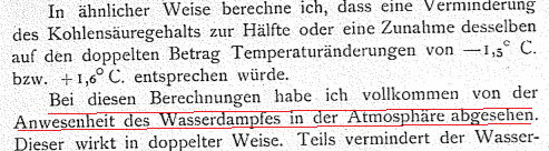
He immediately says (red underline) that the calculation to date ignored the water vapor feedback.
“In these calculations, I completely neglected the presence of water vapour emitted into the atmosphere”
He then goes on to calculate that effect, just as he did in his earlier paper. He concludes

“For this disclosure, one could calculate that the corresponding secondary temperature change, on a 50% fluctuation of CO2 in the air, is approximately 1.8 degrees C, such that the total temperature change induced by a decrease in CO2 in the air by 50% is 3.9 degrees (rounded to 4 degrees C). “
The sensitivity is 4°C per doubling, the result that has been consistently quoted since.
The most recent refutation of this fake story is here
“Guy Stewart Callendar, a British steam engineer, published his own calculation in 1938, and presented his result before the Royal Society (the Society’s subsequent discussion is well worth reading). He, too, predicted 1.6 C° ECS, as the dotted lines I have added to his graph demonstrate:”

This too, does not survive examination of the original, which is
Note the caption, wv 7.5mm Hg. This too is a fixed water vapour content calculation.
Rud Istvan, further up this thread, concludes that Callendar’s estimated ECS was 1.68 K.
Lord Monckton,
If you look up Guy Stewart Callendar on Wikipedia you will find under “Research” that it records his assessment of ECS at 2 degrees Celsius with the remark that this “is on the low end of the IPCC range”.
The authority given is Archer,David and Rahmstorf, Stephan ( 2010) “The Climate Crisis: An Introductory Guide”Cambridge University Press, P.8.
I seem to recall reading at Climate Audit that Stephen McIntyre had reworked Guy Callendar’s papers and come up with an ECS of 1.9C.( perhaps 1.8C,I have lost the link).
So Rud Istvan and 1.68 C looks on the money.
But the sensitivity isn’t 4 K per doubling, for that would imply zero feedback response to emission temperature, which is manifestly nonsense.
Feedback systems are extremely difficult to predict. There are many unsolved problems in this field. Even very simple functions are complex, for instance take function f(x) = 4x(1-x). Plug in random x value between 0 and 1. Keep feeding output f(x) back into function as x. Very different behavior is noticed depending on initial x chosen. Now change 4 to 3.839. In this case for any x initial value between 0 and 1 the iteration settles down to repeating pattern of 3 numbers.
Thanks for the article. But I have to say the way feedbacks are calculated is total absolute codswallop. It really hadn’t occurred to me that anyone would ever try to work out the “feedback” using the approach you describe … it just doesn’t have a physical meaning. If it did, your argument would be sound.
For interest, I wondered what my own atmosphere model produced for a doubling of CO2, and I get 0.56C. However, there are a lot of big assumptions in that figure about how water vapour behaves in the atmosphere.
The two big assumptions, are:
1) how changes in temperature and therefore changes in water vapour then affect cloud density and height
2) What limits the level of water vapour in the atmosphere. There are several models that can be used:
a) Constant energy into evaporation
b) Constant humidity
c) humidity controlled via cloud condensation
There are also some interesting problems in the Stratosphere.
And the assumptions you make about these all will affect the surface temperature change for a doubling of CO2.
Mike Haseler says our professor of control theory is wrong about – er – control theory. Perhaps he would be kind enough to get in touch with me and explain what (aside from one or two misprints) he thinks is wrong with the feedback analysis sketched out in the head posting. He should know that we have also had the assistance of a national laboratory, which has confirmed our conclusions. But perhaps they are all wrong.
I would like it very much if someone could post the actual atmospheric CO2 concentrations that go with various model forecasting scenarios, i.e. for the Hansen predictions, scenarios A, B, and C; for IPCC 4th Assessment, RCP2.6, RCP4.5, RCP6, and RCP8.5; for current model scenarios, the various SSP’s. Only by comparing the track of the CO2 for these scenarios into future time can we tell how closely they relate to what has actual happened. My general impression is that CO2 has continued to increase more like the worst case scenarios than any of them that had significant reductions in CO2 emissions.
https://www.google.com/amp/s/judithcurry.com/2018/07/03/the-hansen-forecasts-30-years-later/amp/
Thanks John.
You’re welcome.
Great post!
Dear Christopher Monckton, your work and findings are highly valuable and will, some day, be appreciated broadly.
About water vapor feedback: I believe the “consensus” principle regarding constant relative humidity is a lazy one. Why isn’t R.H. 100%? Because somehow there’s limited transmission from sources at the earth’s surface or the rate of condensation at top of atmosphere goes up when evaporation increases resulting in lower residence time for each unit of water vapor.
If water feedback was that high they think it is runaways would have happened already…
Earth’s atmosphere is self-stabilizing.
I think I understand the core argument. Using an analogy…
At the end of month 1 you have $1000 in your bank account.
You add $10 and at the end of month 2 you have $1015 in your account.
The incorrect but accepted method of computing interest rate would be that $10 added increased the balance by $15 so there must be a 50% interest rate, ignoring the $1000 starting balance.
Is this an accurate analogy?
Sent from my iPhone
In response to Mr Halland, I think his analogy works, but the danger with analogies is that ex definitione they break down at some point.
So look at it this way. We know that surface temperature with no greenhouse gases in the air at the outset (this is called “emission temperature”) is about 255 K. We know that the temperature in 1850 was 287 K. Therefore, the natural greenhouse effect was 32 K. Of this, about 8 K was direct warming forced by preindustrial noncondensing greenhouse gases. That leaves 24 K total preindustrial feedback response.
Climatology assumes that the 255 K emission temperature engendered no feedback response at all. It assumes that all of the 24 K preindustrial feedback response was driven by the 8 K direct greenhouse-gas warming.
And that is daft. How can 8 K generate a feedback response thrice itself, while 255 K generates no feedback response at all? The truth is that nearly all of the 24 K feedback response was driven by emission temperature, not by the greenhouse-gas warming.
<blockquote>“Climatology . . . assumes that all of the 24 K preindustrial feedback response was driven by the 8 K direct greenhouse-gas warming.” </blockquote>
This is a bald assertion for which Lord Monckton provides no evidence. He’s been flogging the same tired old argument for over three years. Repeating it ad nauseam doesn’t make it any more compelling.
The literature Lord Monckton refers to is largely silent about the feedback to the sun’s radiation because the feedback to the sun and the pre-industrial CO2 is (at least assumed to be) already known, so there’s no need to tease out how much of the existing feedback was attributable to which constituent. All that’s of interest is how much additional feedback results from the additional CO2. This doesn’t imply that only CO2 causes feedback.
I explained all this at https://wattsupwiththat.com/2019/07/16/remystifying-feedback/. II summarized that (admittedly long and mathematical) post as follows:
“Christopher Monckton agrees with heavy hitters like Lindzen & Choi that ECS is low. But Lord Monckton says of such researchers that they ‘can’t absolutely prove that they’re right.’ In contrast, ‘we think that what we’ve done here is to absolutely prove that we are right.’
“His absolute proof’s premise? A fact that he says is ‘well established in control theory but has, as far as we can discover, hitherto entirely escaped the attention of climatology’. Specifically, it’s that ‘such feedbacks as may subsist in a dynamical system at any given moment must perforce respond to the entire reference signal then obtaining, and not merely to some arbitrarily-selected fraction thereof.’ He then contends that if this alleged controls-theory tenet ‘is conceded, as it must be, then it follows that equilibrium sensitivity to doubled CO2 must be low.’”
“We demonstrate that, on the contrary, a low ECS value doesn’t necessarily follow from that tenet. We calculate and display the behavior of a dynamical system that not only exhibits a high ECS value but also a tipping point even though the feedbacks that ‘subsist’ in it ‘at any given moment . . . respond to the entire reference signal then obtaining.’”
Mr Born continues to snipe, to no good effect. He refers us back to a long, rambling, diffuse and delightfully wrong-headed posting that he had written a couple of years ago – but he somehow failed to mention that I had answered that silly posting. The res of my response was that Mr Born had not realized the implications of his analysis, which were that feedbacks would respond 90 times more energetically to each degree of greenhouse-gas warming than to each degree of emission temperature.
Mr Born cannot bring himself to read the references in the head posting, or he would not have attempted to assert, falsely and mendaciously as usual, that I had not provided any evidence that official clahmatawlagy imagines that one-quarter of the greenhouse effect – the direct or reference sensitivity – drives a feedback response amounting to the other three-quarters, giving a system-gain factor 4. Yet there was a quotation from a paper saying precisely that, and, for good measure, that paper went on to state that the system-gain factor was 4, which it could only have been if no account had been taken of the large feedback response to the emission temperature.
Next, Mr Born waffles to the effect that climatological papers don’t mention the feedback response to emission temperature because “it is known”. Here, Mr Born catches himself on a Morton’s Fork that all who are not really interested in the objective truth will impale themselves upon.
It is, of course, quite evident from the numerous citations in the head posting that climatology takes no account whatsoever of any feedback response to emission temperature. If Mr Born thinks otherwise, let him find even a single climatological paper that quantifies it and accordingly reduces the preindustrial system-gain factor from the currently-estimated 4 to something a lot smaller.
For if climatology had taken due account of the feedback response to emission temperature, it would not have predicted a system-gain factor as great as 4, unless it made the same mistake that Mr Born unfortunately made in his earlier article – of implicitly assuming a unit-feedback-response ratio that is so excessive as to be untenable.
Mr Born has also failed to appreciate that official climatology treats unit feedback response as near-invariant with temperature, so, in maundering on about nonlinearities, he is criticizing not us but official climatology.
By the method of taking due account of the feedback response to emission temperature, we derive a system-gain factor ~1 for the preindustrial era.
By the entirely distinct energy-balance method, using the latest climatological data, we derive a system-gain factor ~1 for the industrial era. Not much nonlinearity there, then.
Recall that we have the advantage of a more than usually competent professor of control theory, who keeps us straight on his specialist subject. Mr Born has no relevant qualifications or experience, and is unfortunately very much out of his depth.
He has been attempting – and lamentably failing – to prove us wrong ever since he was caught out in a series of outright falsehoods. It seems the Born Liar is still at it.
Showing that Lord Monckton’s theory is just bad extrapolation and that it wouldn’t “check out” in an electronic “test rig.”:
https://wattsupwiththat.com/2021/05/11/an-electronic-analog-to-climate-feedback/
The reason why the ensemble models don’t predict temperature correctly is they all have ‘way too high ECS entered into them, except the Russian INM-CM4 model. The Russians don’t give much truck to the climate activists, so they could actually model climate not write what otherwise is basically a fantasy computer game.
The trouble for the climate activists is wicked though. They can’t include a realistic ECS because if they did that it would prove global warming is harmless.
And if they proved global warming is harmless they’d all lose their jobs when the funding was withdrawn.
We have to fight climate change now. Its an emergency. But since climate is 30 years of average weather, we have to fight weather for 30 years first. You can’t fight the weather that happened in the past. But winning the fight against weather means you have to control the weather. Good luck with that. I heard dancing and tossing virgins into volcanoes doesn’t work.
Arrhenius wasn’t the first to attempt to predict eventual warming by doubled CO2. I believe that honour goes to John Tyndal in 1859. Even then he wasn’t the first to make the climate link. “That prize goes to the American Eunice Foote, who showed in 1856 using sunlight that carbon dioxide could absorb heat. She suggested that an increase in carbon dioxide would result in a warmer planet.” https://theconversation.com/john-tyndall-the-forgotten-co-founder-of-climate-science-143499#:~:text=In%201859%2C%20Tyndall%20showed%20that,emanating%20from%20the%20Earth's%20surface.
Arrhenius was the first to attempt to quantify ECS.
Christopher,
Thank you again for this important contribution.
Again, you emphasise that the feedback has to be calculated on the actual temperature, not a constructed change in temperature. Along similar lines, I have been pondering if they are even using the proper temperature metric.
This is a long and technical posting. If you don’t want to read it, my bad luck.
…………………………..
To provide a neat example, the Australian BOM produced an Annual Climate Statement for year 2020.
http://www.bom.gov.au/climate/current/annual/aus/2020/annual-summary-table.shtml
From its Table of annual rainfall, temperature and sea surface temperature this graph was prepared.http://www.geoffstuff.com/temp_rain.jpg
The graph shows an inverse statistical relation between annual temperature and annual rainfall. In short, rain cools, as expected from known physics of evaporation, sensible and latent heat, etc..
For example, wet bulb thermometers and conventional dry bulb temperatures produce correlated, but dissimilar measurements at the same place and time. Climate analysts have uses for both. Both temperatures are affected by water, one on the bulb and the other in the nearby ground and air. Yet, for expression of temperatures, climate analysts have concentrated mainly on uncorrected-for-rain near-surface temperatures from dry bulb thermometers in surrounds like Stevenson screens.
For an analogy, a surveyor can run a metal tape between 2 points to measure their separation. The metal tape is known to expand with heat. Therefore, a correction is applied for expansion after
Should climate analysis continue to be based on this dry bulb temperature or on a more fundamental version of it corrected for the effect of rainfall? Should rainfall be regarded as a forcing or a feedback that affects the customary temperature?
With regard to physics, The Stefan-Boltzmann law is expressed as W = σT4, where W is the radiant energy emitted per second and per unit area and the constant of proportionality is σ = 0.136 calories per metre2-second-K4. Which is the appropriate temperature to represent T in this equation, the measured-in-practice T or that T corrected for the variable, rainfall? There are significant differences between these, especially when raised to the power of four.
Are current modellers using the wrong temperature metric in physics equations?
Yes, we know what is used mostly, for no better reason than it is was collected historically. But it is wrong. Geoff S
Christopher M – Many thanks for yet another lucid article, though I would have to say that this one excels in lucidity.
A correction (apologies if already picked up by others): “The system-gain factor is then 287 / (255 + 32), or 1.09” should be “The system-gain factor is then 287 / (255 + 8), or 1.09”. It doesn’t affect your analysis.
Many thanks to Mike Jonas for his very kind comments. We have been working hard on keeping the argument very simple. Of course, there are dangers in that approach. For Al Gore’s Komsomol training camps for Thermageddonite fanatics train them to address every serious challenge to the Party Line on climate by saying 1) that the nonlinearities have not been correctly taken into account; 2) that the uncertainties have not been correctly taken into account; and 3) that the complexities have not been correctly taken into account.
At root, though, climatology’s error is a very simple one. And it is increasingly giving peer-reviewers of our paper a headache. On the last two occasions on which it was submitted, the reviewers were not able to dent the main point at all. On the second occasion, one of the reviewers actually wrote that he had read our conclusions, had not liked them and had not, therefore, bothered to read the arguments justifying them. And that was all that his review said.
Our paper has now been before the current journal for six months. If there had been anything as obviously wrong with our argument as one or two of the usual suspects here have tried to suggest, it would have been thrown back at us by now.
“eventual warming by doubled CO2, known to the crystal-ball gazers as equilibrium doubled-CO2 sensitivity (ECS)”
ECS is just the correlation between global mean surface temperature and the logarithm of atmospheric CO2 concentration, not really an “eventual warming by doubled CO2”.
For the 270ppm of pre industrial CO2 to double we would have to wait until it gets to 540 ppm for the doubling measurement.
The time scale for this effect is usually stated as 60+ years so you don’t really have to wait for the CO2 concentration to double to measure ECS. That’s what I thought anyway. I could be wrong I guess.
Correction. Not the correlation but the regression coefficient. That coefficient is the ecs. The correlation or the coefficient, if statistically significant, supports the validity of the ecs.
Thanks, enlightening (what I could follow at least). Question on this:
“Why, then, do the models get their predictions so wrong? In the medium term (top of the diagram below), midrange projected anthropogenic medium-term warming per century equivalent was 3.4 K as predicted by IPCC in 1990, but observed warming was only 1.65 K, of which only 70% (Wu et al. 2019), or 1.15 K, was anthropogenic. IPCC’s prediction was thus about thrice subsequently-observation, in line with the error but not with reality.”
What basis, and who’s was there to claim that the 1.15 was anthropogenic?
Thanks
In response to JBP, Wu et al. (2019), in preparation for AR6, wrote a paper that – instead of dopily counting heads among clahmatawlagists, actually made the attempt to quantify the anthropogenic contribution to warming since 1850 and concluded that it was 70% of the total, the rest being natural.
Our approach is to accept all of official climatology ad argumentum except what we cannot prove to be false, so we use the 70% value.
The models used in the IPCC 2013 report, CMIP5 I think, seem to be doing quite well.
http://blogs.reading.ac.uk/climate-lab-book/files/2021/01/fig-nearterm_all_UPDATE_2020.png
Well, any fool can do a naive extrapolation of recent temperature trends and be in the right ballpark only seven years after the original prediction was made. However, the graph to which TheFinalNail refers stops at the beginning of 2020 and does not, therefore, capture the sharp recent decline in temperatures as the La Nina takes effect.
The truth is that the original IPCC medium-term predictions of anthropogenic warming – the ones that got the climate scare going – have proven to be 2.4 times what has actually happened. The head posting explains why it is that the models are running hot.
As Dr John Christy has recently demonstrated, the models are running hot in the lower troposphere, in the mid-troposphere, in the bulk troposphere and over the sea surface. Wherever you look, reality has not matched prediction. And they’re not just running a little hot – they’re predicting about three times as much medium-term warming as is occurring.
One can only make them appear to fit reality by comparing very short prediction timeframes with observation – as the Reading graph does.
Your nail is getting a little rusty. You forgot to remove the noise. Hence, your chart is meaningless nonsense as a measure of real warming. A good way to remove noise is to look for periods that are reasonably similar. For example, both 2001 and 2021 are years where we have +PDO, +AMO and coming out of La Nina events.
If we look at combined March and April anomalies from UAH satellite data, they are 0.00 and -0.03 over those two months. Essentially, no warming at all.
Another good comparison year is 1990 which also saw La Nina conditions as the last ENSO event. The two month anomaly was -0.13. However, that was back when we had a -AMO.
The total warming comes to about 0.1 C over the time your models projected nearly 1 C. They are off by at least a factor of 10 when you consider the AMO change.
How can models work if they have not included the observations by the British meteorologist A.J. Drummond in 1943*):: :
· “The present century has been marked by such a widespread tendency towards mild winters that the ‘old-fashioned winters’, of which one had heard so much, seemed to have gone forever”.
· The sudden arrival at the end of 1939 of what was to be the beginning of a series of cold winters was therefore all the more surprising. (underline added)
· “Never since the winters of 1878/79, 1879/80 and 1880/81 have there been in succession three so severe winters as those of 1939/40, 1940/41 and 1941/42.”
· “Since comparable records began in 1871, the only other three successive winters as snowy as the recent ones (1939/40, 1940/41 1941/42) were those during the last war, namely 1915/16, 1916/17 and 1917/18…”. ,
*) Drummond, A. J.; (1943); “Cold winters at Kew Observatory, 1783-1942”; Quarterly Journal of Royal Met. Soc., No. 69, pp. 17-32, and ibid; Discussion: “Cold winters at Kew Observatory, 1783-1942”; Quarterly Journal of Royal Met. Soc., 1943, p. 147ff
Discussed in a recent post at: https://oceansgovernclimate.com/the-first-climate-criminal-adolf-hitler-1889-1945/