Reposted from Dr. Roy Spencer’s Blog
February 5th, 2020 by Roy W. Spencer, Ph. D.
Note: What I present below is scarcely believable to me. I have looked for an error in my analysis, but cannot find one. Nevertheless, extraordinary claims require extraordinary evidence, so let the following be an introduction to a potential issue with current carbon cycle models that might well be easily resolved by others with more experience and insight than I possess.
Summary
Sixty years of Mauna Loa CO2 data compared to yearly estimates of anthropogenic CO2 emissions shows that Mother Nature has been removing 2.3%/year of the “anthropogenic excess” of atmospheric CO2 above a baseline of 295 ppm. When similar calculations are done for the RCP (Representative Concentration Pathway) projections of anthropogenic emissons and CO2 concentrations it is found that the carbon cycle models those projections are based upon remove excess CO2 at only 1/4th the observed rate. If these results are anywhere near accurate, the future RCP projections of CO2, as well as the resulting climate model projection of resulting warming, are probably biased high.
Introduction
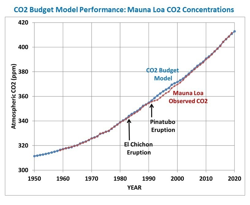
My previous post from a few days ago showed the performance of a simple CO2 budget model that, when forced with estimates of yearly anthropogenic emissions, very closely matches the yearly average Mauna Loa CO2 observations during 1959-2019. I assume that a comparable level of agreement is a necessary condition of any model that is relied upon to predict future levels of atmospheric CO2 if it is have any hope of making useful predictions of climate change.
In that post I forced the model with EIA projections of future emissions (0.6%/yr growth until 2050) and compared it to the RCP (Representative Concentration Pathway) scenarios used for forcing the IPCC climate models. I concluded that we might never reach a doubling of atmospheric CO2 (2XCO2).
But what I did not address was the relative influence on those results of (1) assumed future anthropogenic CO2 emissions versus (2) how fast nature removes excess CO2 from the atmosphere. Most critiques of the RCP scenarios address the former, but not the latter. Both are needed to produce an RCP scenario.
I implied that the RCP scenarios from models did not remove CO2 fast enough, but I did not actually demonstrate it. That is the subject of this short article.
What Should the Atmospheric CO2 Removal Rate be Compared To?
The Earth’s surface naturally absorbs from, and emits into, the huge atmospheric reservoir of CO2 through a variety of biological and geochemical processes.
We can make the simple analogy to a giant vat of water (the atmospheric reservoir of CO2), with a faucet pouring water into the vat and a drain letting water out of the vat. Let’s assume those rates of water gain and loss are nearly equal, in which case the level of water in the vat (the CO2 content of the atmosphere) never changes very much. This was supposedly the natural state of CO2 flows in and out of the atmosphere before the Industrial Revolution, and is an assumption I will make for the purposes of this analysis.
Now let’s add another faucet that drips water into the vat very slowly, over many years, analogous to human emissions of CO2. I think you can see that there must be some change in the removal rate from the drain to offset the extra gain of water, otherwise the water level will rise at the same rate that the additional water is dripping into the vat. It is well known that atmospheric CO2 is rising at only about 50% the rate at which we produce CO2, indicating the “drain” is indeed flowing more strongly.
Note that I don’t really care if 5% or 50% of the water in the vat is exchanged every year through the actions of the main faucet and the drain; I want to know how much faster the drain will accomodate the extra water being put into the tank, limiting the rise of water in the vat. This is also why any arguments [and models] based upon atomic bomb C-14 removal rates are, in my opinion, not very relevant. Those are useful for determining the average rate at which carbon cycles through the atmospheric reservoir, but not for determining how fast the extra ‘overburden’ of CO2 will be removed. For that, we need to know how the biological and geochemical processes change in response to more atmospheric CO2 than they have been used to in centuries past.
The CO2 Removal Fraction vs. Emissions Is Not a Useful Metric
For many years I have seen reference to the average equivalent fraction of excess CO2 that is removed by nature, and I have often (incorrectly) said something similar to this: “about 50% of yearly anthropogenic CO2 emissions do not show up in the atmosphere, because they are absorbed.” I believe this was discussed in the very first IPCC report, FAR. I’ve used that 50% removal fraction myself, many times, to describe how nature removes excess CO2 from the atmosphere.
Recently I realized this is not a very useful metric, and as phrased above is factually incorrect and misleading. In fact, it’s not 50% of the yearly anthropogenic emissions that is absorbed; it’s an amount that is equivalent to 50% of emissions. You see, Mother Nature does not know how much CO2 humanity produces every year; all she knows is the total amount in the atmosphere, and that’s what the biosphere and various geochemical processes respond to.
It’s easy to demonstrate that the removal fraction, as is usually stated, is not very useful. Let’s say humanity cut its CO2 emissions by 50% in a single year, from 100 units to 50 units. If nature had previously been removing about 50 units per year (50 removed versus 100 produced is a 50% removal rate), it would continue to remove very close to 50 units because the atmospheric concentration hasn’t really changed in only one year. The result would be that the new removal fraction would shoot up from 50% to 100%.
Clearly, that change to a 100% removal fraction had nothing to do with an enhanced rate of removal of CO2; it’s entirely because we made the removal rate relative to the wrong variable: yearly anthropogenic emissions. It should be referenced instead to how much “extra” CO2 resides in the atmosphere.
The “Atmospheric Excess” CO2 Removal Rate
The CO2 budget model I described here and here removes atmospheric CO2 at a rate proportional to how high the CO2 concentration is above a background level nature is trying to “relax” to, a reasonable physical expectation that is supported by observational data.
Based upon my analysis of the Mauna Loa CO2 data versus the Boden et al. (2017) estimates of global CO2 emissions, that removal rate is 2.3%/yr of the atmospheric excess above 295 ppm. That simple relationship provides an exceedingly close match to the long-term changes in Mauna Loa yearly CO2 observations, 1959-2019 (I also include the average effects of El Nino and La Nina in the CO2 budget model).
So, the question arises, how does this CO2 removal rate compare to the RCP scenarios used as input to the IPCC climate models? The answer is shown in Fig. 1, where I have computed the yearly average CO2 removal rate from Mauna Loa data, and the simple CO2 budget model in the same way as I did from the RCP scenarios. Since the RCP data I obtained from the source has emissions and CO2 concentrations every 5 (or 10) years from 2000 onward, I computed the yearly average removal rates using those bounding years from both observations and from models.
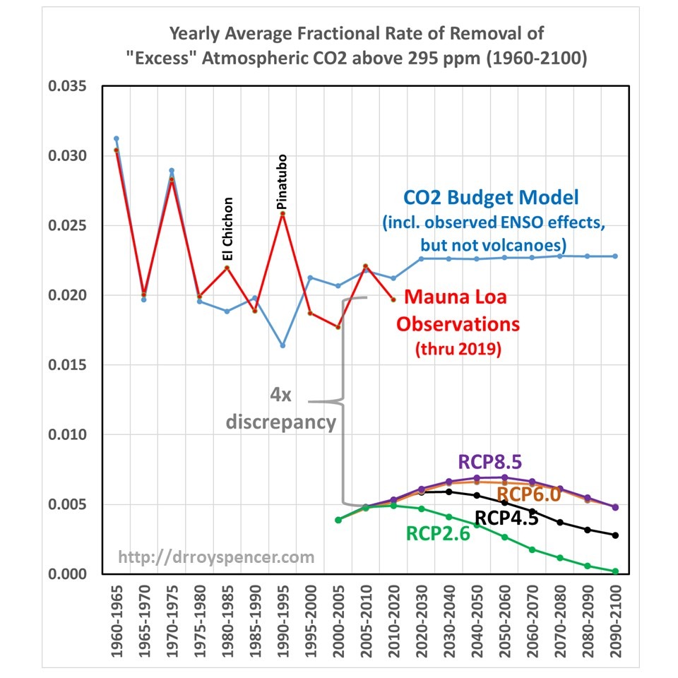
Fig. 1. [fixed] Computed yearly average rate of removal of atmospheric CO2 above a baseline value of 295 ppm from historical emissions estimates compared to Mauna Loa data (red), the RCP scenarios used by the IPCC CMIP6 climate models, and in a simple time-dependent CO2 budget model forced with historical emissions before, and assumed emissions after, 2018 (blue). Note the time intervals change from 5 to 10 years in 2010.
The four RCP scenarios do indeed have an increasing rate of removal as atmospheric CO2 concentrations rise during the century, but their average rates of removal are much too low. Amazingly, there appears to be about a factor of four discrepancy between the CO2 removal rate deduced from the Mauna Loa data (combined with estimates of historical CO2 emissions) versus the removal rate in the carbon cycle models used for the RCP scenarios during their overlap period, 2000-2019.
Such a large discrepancy seems scarcely believable, but I have checked and re-checked my calculations, which are rather simple: they depend only upon the atmospheric CO2 concentrations, and yearly CO2 emissions, in two bounding years. Since I am not well read in this field, if I have overlooked some basic issue or ignored some previous work on this specific subject, I apologize.
Recomputing the RCP Scenarios with the 2.3%/yr CO2 Removal Rate
This raises the question of what the RCP scenarios of future atmospheric CO2 content would look like if their assumed emissions projections were combined with the Manua Loa-corrected excess CO2 removal rate of 2.3%/yr (above an assumed background value of 295 ppm). Those results are shown in Fig. 2.
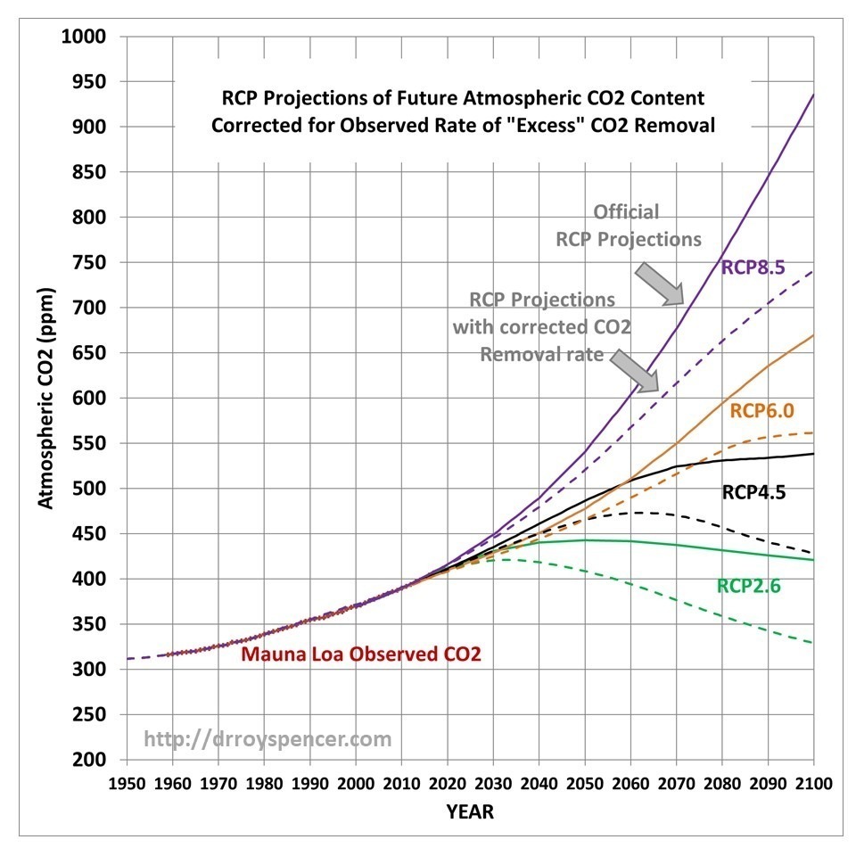
Fig. 2. Four RCP scenarios of future atmospheric CO2 through 2100 (solid lines), and corrected for the observed rate of excess CO2 removal based upon Mauna Loa data (2.3%/yr of the CO2 excess above 295 ppm, dashed lines).
Now we can see the effect of just the differences in the carbon cycle models on the RCP scenarios: those full-blown models that try to address all of the individual components of the carbon cycle and how it changes as CO2 concentrations rise, versus my simple (but Mauna Loa data-supportive) model that only deals with the empirical observation that nature removes excess CO2 at a rate of 2.3%/yr of the atmospheric excess above 295 ppm.
This is an aspect of the RCP scenario discussion I seldom see mentioned: The realism of the RCP scenarios is not just a matter of what future CO2 emissions they assume, but also of the carbon cycle model which removes excess CO2 from the atmosphere.
Discussion
I will admit to knowing very little about the carbon cycle models used by the IPCC. I’m sure they are very complex (although I dare say not as complex as Mother Nature) and represent the state-of-the-art in trying to describe all of the various processes that control the huge natural flows of CO2 in and out of the atmosphere.
But uncertainties abound in science, especially where life (e.g. photosynthesis) is involved, and these carbon cycle models are built with the same philosophy as the climate models which use the output from the carbon cycle models: These models are built on the assumption that all of the processes (and their many approximations and parameterizations) which produce a reasonably balanced *average* carbon cycle picture (or *average* climate state) will then accurately predict what will happen when that average state changes (increasing CO2 and warming).
That is not a given.
Sometimes it is useful to step back and take a big-picture approach: What are the CO2 observations telling us about how the global average Earth system is responding to more atmospheric CO2? That is what I have done here, and it seems like a model match to such a basic metric (how fast is nature removing excess CO2 from the atmosphere, as the CO2 concentration rises) would be a basic and necessary test of those models.
According to Fig. 1, the carbon cycle models do not match what nature is telling us. And according to Fig. 2, it makes a big difference to the RCP scenarios of future CO2 concentrations in the atmosphere, which will in turn impact future projections of climate change.
Just like we were surprised to see how much CO2 nature has absorbed, we will be equally amazed how much more can be absorb. Mother Nature is amazingly resilient. We are learning new things everyday, and I thank Roy for quantifying and graphing current thinking. While not limitless, we now know nature’s ability to “sink” excess CO2 is huge, and to put it in “alarmist rhetoric” … nature’s CO2 sinks are alarmingly efficient.
With respect to CO2 consumption, is the planetary plant world a linear model? Are greenhouses even linear? I think nature has a few surprises that fossils and geochemistry cannot fully explain.
In theory maybe, in practice, never. Photosynthesis has limiting factors such as water for example. And of course sunlight.
First off, it is clear the BernSCM v1.0 CO2 model presented in this paper…
“The Bern Simple Climate Model (BernSCM) v1.0: an extensible and fully documented open-source re-implementation of the Bern reduced-form model for global carbon cycle–climate simulations” (by Kuno M. Strassmann and Fortunat Joosat University of Bern, Bern, Switzerland)
https://www.geosci-model-dev.net/11/1887/2018/
is a failure. It is simpler construct of earlier more complex Bern model of carbon cycle.
It was a failure while it was under-review in late 2017 before it was published in 2018. It is utterly wrong. Yet it is what the IPCC and the consensus establishment needs to maintain the climate scam on human FF emissions –> atmospheric CO2 growth (MLO record) –> LWIR forcing growth –> temperature and everything else they claim.
A very simple demonstration of the crux of this paradigm failure can be seen in this NOAA/ESRL data graphic:
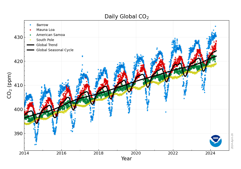
Note the Barrow Alaska seasonal dynamic range ~22 ppm, peak to trough. The trough (the summer low pt) is in August, the peak of Arctic heating and near sea ice minimum. Yet with all that “warming exposed” seawater and exposed decaying tundra, CO2 is falling very rapidly across the Arctic.
Another informative graphic to show what is happening is this detrended seasonal cycle and the smoothed curve (red).
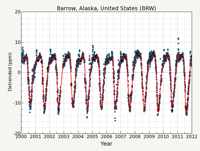
This detrended graphic stops at 2012, but it shows in 2000, the seasonal swing was (roughly) 15.5 ppm (red, smoothed line), but by 2011 that seasonal swing had increased to almost 20 ppm. And back to the previous graph, you can see that the 2019 seasonal swing was almost 22 ppm at Barrow.
Conclusions: The high latitude biosphere is being highly productive and not only taking in lots of CO2 , it’s summer time drawdown rate is increasing, even as the Arctic has warmed. Not inspite of the warming, but probably EXACTLY because the Arctic has warmed has this drawdown increased over the last 2 decades. Even though more warming summer open water should, from a purely geophysical standpoint, be outgassing more CO2 with each year, that is not what appears to be happening.
This is the opposite behavior predicted by the Bern Model for a warming high latitudes of the Arctic. The Bern Model is failure but the IPCC’s AR6 WG1 report will most certainly base all its emissions-CO2 growth scenarios on in their CMIP6 model runs. That’s IPCC junk science at work.
Quote: “Even though more warming summer open water should, from a purely geophysical standpoint, be outgassing more CO2 with each year, that is not what appears to be happening.”
The common understanding is that the open high-latitude ocean waters absorb CO2 and the warm tropical waters absolve CO2. Could an explanation be that´more open ocean water increases the CO2 absorption?
Yes, more open water is not just a chemical sink (Henry’s Law), but also the biological productivity is greatly increasing. More phytoplankton, more CO2 sequestration.
“Phytoplankton Blooms are Moving into New Territory in the Arctic Ocean.”
https://e360.yale.edu/digest/phytoplankton-blooms-are-moving-into-new-territory-in-the-arctic-ocean
and the study itself:
Northward Expansion and Intensification of Phytoplankton Growth During the Early Ice‐Free Season in Arctic
https://agupubs.onlinelibrary.wiley.com/doi/full/10.1029/2018GL078995
The authors admit this in their discussion regarding the phytoplankton spring bloom (PSB):
“At the highest latitude (i.e., >80°N), the PSB develops around early September (on average the 250th day of year, result not shown). “
NH summer solstice is day 172 (June 21). So this high latitude PSB is happening 78 days after peak sun angle, and the days are rapidly shrinking, air temperatures are beginning to fall and hard freezes return starting in mid-August, with a low a sun angle at day 250 (~7 September). 2 weeks around that date are when Barrow CO2 data shows drawdown (sink) rate is peaking. Clearly this is biological drawdown of immense proportions.
Plants in a glass house which are supplied by a level controlled reservoir shows water consumption responds to changes in cloud cover on a sunny day within 15 minutes. When a cloud passes over the greenhouse water consumption declines and when the sun shines again , it increase. On oceans where UV is high , phytoplankton could increase photosynthesis within 15 minutes. I would suggest one would need a geostationary satellite taking images every 15 minutes to measure plankton growth. Where there are rapid fluctuations plankton will probably store starch but not necessarily increase in numbers. Consequently, two different plankton could contain different levels of carbons. How deep within the oceans do plankton exist and how deep can the measurement be made ?
A satellite may measure coverage of plants but it will not measure total mass of roots. Most plants in arid and sem-arid areas use roots for storage. Often only experienced Bush people can recognise that beneath a small withered stick lies succulent water and carbohydrate bearing roots.
in summary, rapid increases in food supply encourage organisms to lay down reserves. Only only when there is prolonged increase in food supply do organisms reproduce.
In general, computer modellers have taken over from scientists with field experience.
This should come as no real surprise given the rapidity and degree of seasonal decline in atmospheric carbon dioxide. It’s good to see my suspicions are justified as the mathematics is well beyond me. Will this finding also be ignored by climate alarmists or is that just another of my suspicions?
Another factor to consider. Photosynthesis reaction rate increases with increasing CO2 concentration
Hi Mike McHenry, – The effect of elevated CO2 (eCO2) is not simply a linear increase in carbon assimilation (how fast leaves photosynthesized). I will cite an example of what relates to rate of photosynthesis gauged by it’s results; it is for a tree, so am not declaring a dynamic for crops (although suspect some extrapolation of the dynamic is likely).
At ambient CO2 8 years old European Beach trees during the morning on sunny days assimilated an average of 14.8 microMoles CO2/sq.mt./sec & during afternoons on sunny days assimilated an average of 16.2 microMoles CO2/sq.mt./sec.
During sunny days eCO2 definitely did allow the same kind of trees to perform more photosynthesis is the same amounts of time. During sunny mornings an average of 17.8 microMoles C02/sq.mt./sec. was assimilated & during sunny afternoons an average of 21.5 microMoles CO2/sq.mt./sec. was assimilated.
The eC02 average sunny days total assimilation was 72 Moles CO2/sq.mt./day. Which is more than the ambient CO2 average sunny days assimilation total of 53.5 Moles CO2/sq.mt/day.
However, under cloudy conditions the photosynthetic results reversed. Then eCO2 during cloudy mornings only an average of 9.8 microMoles CO2/sq.mt/sec. was assimilated; verses 12.3 microMoles CO2/sq.mt/sec. at ambient CO2 on cloudy mornings.
And likewise counter-intuitively during cloudy afternoons ambient CO2 was performing even more photosynthesis by assimilating an average of 15.7 microMoles CO1/sq.mt./sec.; verses 9.4 microMoles CO2/sq.mt./sec. at eCO2 on cloudy afternoons.
During cloudy days the tees grown at ambient CO2 assimilated an average of 26.7 Moles/ CO2/sq.mt/day. Which is more than the average 17.5 Moles CO2/sq.mt/day they assimilated under eCO2.
As per (2014) “Impact of elevated CO2 concentration on dynamics of leaf photosynthesis in Fagus sylvatica is modulated by sky conditions”; free full text with much more data available on-line.
RCP8.5 includes permafrost melting effects and that is one reason for a very high CO2 increase in the atmosphere. The question is if that is it a realistic scenario to be called “Business as usual”. The BAU scenario is much closer to the present CO2 growth rate.
Antero,
I make no claims regarding this, but pass it along for reading:
Worst emissions scenarios “exceedingly unlikely” (RCP 8.5)
https://www.bbc.com/news/science-environment-51281986
That assumption is why the RCP is so flawed. The assumption that CO2 will go up if permafrost melts is bass-ackwards. If permafrost melts, trees grow rapidly in the space available. This is easily demonstrated by pointing out that centuries ago all of central Canada was permafrost and now it is covered with forests (where it is warm enough).
The “methane bomb” was supposed to arise from the same permafrost areas, but it turns quickly into CO2 and is absorbed by the new tree growth. Think for a moment about where the methane comes from – the rotting of vegetation currently frozen in the ice. Well…where did it come from? It grew there the last time it was much warming than now, a few thousand years ago.
Nuff said.
Crispin,
I think that the concern about permafrost is from the deposits in Siberia, not Canada. In Canada, the glaciers removed all the ground cover so there can only be a few thousand years of material there. Siberia wasn’t covered by glaciers during the most recent glaciation.
I used Ernst Georg Beck’s data to argue the average CO2 level was 360 ppm in the 1800’s and there were spikes to 550 ppm in 1825 and 1942. One Alarmist argued back that nobody accepted Becks graphs because he couldn’t provide the means by which the CO2 level fell back to normal in such a short period of time. If this article is correct then IMHO that objection to Beck’s work has been answered. I also remember reading another article a few years ago that the global tree inventory had been underestimated fourfold. That makes me suspect the IPCC might not have updated their models to correct for that miscalculation.
Beck’s measurements are of localized CO2 levels that are not representative of overall atmospheric CO2. One reason this happens is that the surface-level atmosphere in and shortly downwind of land areas with active biomass can deviate significantly from overall atmospheric CO2 due to regional sourcing/sinking of CO2. This regional deviation of surface-level and near-surface CO2 has some tendency to have a unidirectional component, upwards. This happens because when the biomass is sinking CO2, there is usually sunlight and the surface-level air is usually mixing with the air in the kilometer or two above the surface due to convection, and when the biomass is sourcing CO2 there is often little or no sunlight and convection is less likely.
Chris Hoff,
Sorry, but there were no CO2 spikes in at least 1942, which I have thoroughly examined and discussed with the late Ernst Beck.
The problem is not the measurements which were reasonably accurate, the problem is where was measured: in the middle of towns, vegetation,… Where you can find any level from 250 to 500 ppmv, depending of wind speed, time of the day, traffic,…
See: http://www.ferdinand-engelbeen.be/klimaat/beck_data.html
Nevertheless, the removal rate of the extra CO2 in the atmosphere above the long time equilibrium between ocean surface and atmosphere for the average ocean surface temperature is quite linear.
My other debate point was the NASA water vapor survey. The one that combined 4 weather balloon studies and satellite data, showing a 1% drop in upper atmosphere water vapor over the last 40 years and argued this would cause more cooling than warming. Perhaps as the water vapor declines it’s pulling down the extra CO2 with it.
Chris Hoff,
I have no point on that, only that CO2 and water vapor act independent of each other and that the solubility of CO2 in fresh water drops/clouds/rain at 0.0004 atm pCO2 is extremely low…
If condensed out of a lot of m3 of air, the difference in CO2 level would be too small to measure.
If these drops fall on the surface, the local CO2 level in the first meter may increase with 1 ppmv if all that water evaporates and the dissolved CO2 is set free…
The concentration in the northern hemisphere falls rapidly between seasons. Why is it so hard to believe that the warming from the very cold period around 1815 was not over and all the plants grew better?
The situation described in the post makes excellent sense when the entire biosphere is considered. I recently did a review of the past research on some of the primary crop plants and most common tree species to find out what the optimal atmospheric CO2 concentrations were for these species. The optimal level was consistently between 750 and 1000 ppm. Some phytoplankon species go much higher.
It would appear that current CO2 levels and higher should dramatically increase plant growth, and both balance future emissions and provide food and products for humanity’s needs in the future. Perhaps we should focus on removing pollution and ignore CO2. Labeling CO3 as a pollutant was a very ignorant and ridiculous step.
The Earth is greening and even the Joos et al. (2013) accepts this as a fact. Otherwise, they cannot close the carbon budget. It has been estimated that the present higher CO2 concentration has increased crops by 10-15 %. During recent years all-time high crops have been reported from the warmest countries like India, Brazil, and Egypt.
That shouldn’t surprise anyone, ….. given the fact estimates of yearly anthropogenic emissions were formulated specifically to match with the yearly average Mauna Loa CO2 observations. “DUH”, no one ever estimated yearly anthropogenic emissions until a few years after Keeling provided them a “target” to shoot at.
And it makes no matter anyway because yearly anthropogenic CO2 emissions are surely less than 5% of all CO2 emissions into the atmosphere.
The fact of the matter is, iffen the earth was not “tilted” on its axis ….. there would not be a biyearly (seasonal) cycling of an average 6 ppm atmospheric CO2 as defined by the KC Graph.
“The CO2 budget model I described here and here removes atmospheric CO2 at a rate proportional to how high the CO2 concentration is above a background level nature is trying to “relax” to, a reasonable physical expectation that is supported by observational data.”
I think that is where it goes wrong. It is not a reasonable physical expectation. It says that the 280 ppm of a century ago is somehow enshrined in the physics. Diffusion does not work like that.
The model would be right if the excess CO2 were diffusing through a resistive layer which itself held none of it, into a sink which stayed at the previous equilibrium conditions. But it isn’t like that. At each stage in the ocean the CO2 is diffusing into a region where the CO2 levels have already increased. The concentration gradients are reduced by the accumulation of past diffusion, and so the flux is lowered. Past CO2 influx gets in the way of current influx. And the memory of that past 280 ppm attenuates.
To put it in terms of the faucet/tank/drain model, a diffusion is not just one tank. It is a whole series, with each draining into the next. And the drain flux is proportional to the pressure difference between tanks. So as the second tank fills up, the first drains more slowly, and so on down. The pathway is more resistive than one where the tanks drains into an infinite sink.
If the sinks were all geophysical your point is a valid concern on the filling of sinks and ultimately saturating and a decreasing sink flux.
But that is not what is happening. The Earth of course is not a sterile geosphere. There is quite significant consumer of CO2 at play. Seasonal CO2 flux rates are increasing. Clearly the biological sinks are kicking in drawing down ever higher amounts of carbon to be sequestered, either into the food chain (greening the biosphere), or to sink in to the ocean depths as dissolved organic carbon, or as sequestered-decaying organic matter on land (like the high Arctic).
Life has been altering the very nature of this planet for at least ~2.5 billion years and will continue to do so.
The point is the arithmetic of working on the excess. The deep ocean does have a memory of the 280 ppm that it was in equilibrium many years ago, so there is some basis for relating change to the excess. But not with a constant resistance, because as time goes on, CO2 has to diffuse further to reach parts where that ancient equilibrium works. That increase the diffusive resistance.
Plants don’t have such a memory (of280) at all. They may have some other non-linear response to rising CO2, but you’d have to work it out. The main thing is that the biosphere is too small to absorb a whole lot more CO2. Our total emission to date is about equal to all the carbon in the biosphere.
The time scale of deep ocean (hundreds of years) will never been seen (separable) on top of the much larger faster biological responses (years, decades).
The ocean has been doing most of the absorption. If plants had absorbed the non-airborne fraction of our emissions, the biomass would have increased by at least 50%, and we would have noticed. The top 100 m of ocean are quite sufficient to absorb that fraction. But as they build up CO2 content, the rate slows.
“The top 100 m of ocean are quite sufficient to absorb that fraction.”
And, more. Much more. It is assumed that they are absorbing only 50% because that is in superficial agreement with observations.
Nick,
Look at the 21st century flux rates at https://www.esrl.noaa.gov/gmd/ccgg/carbontracker/fluxmaps.php?region=asi&average=longterm#imagetable
The scale chosen for the oceans peaks at -30
grams carbon per square meter per year.
Much of both the US and China both have been drawing down significant amounts of CO2 since 2001. The scale for land flux goes down to -120 grams carbon per square meter per year. So on a per square meter basis, land has at least 4x the potential to draw down CO2 than the oceans.
Other detail level studies have shown much (50%?) of US and China’s drawdown is taking place on cropland. Newly formed forests also have a significant drawdown, especially in China where large amounts of new forests exist.
Cropland by definition has no annual increase in above ground biomass. That is only annual plants are grown and above ground biomass effectively returns to zero at least once a year.
That leaves soil organic carbon as the repository that is accumulating much of the carbon being drawn down from the atmosphere.
While global biomass is around 550 GT carbon, the global soil carbon repository is about 2,000 GT carbon in the top meter of soil and about 3,000 GT carbon in the top 2 meters of soil. The current atmospheric carbon surplus above 1850 is 250-300 GT carbon, so the top 2 meters of soil holds 10x the atmospheric carbon increase since 1850.
[Accuracy on the global soil carbon estimate is very poor, so adding another digit to the estimate is a false significant digit.]
Anyway, a truly large and underappreciated carbon flux is from the atmosphere into plants and then from plants into the soil. And agricultural soil under the management of US and Chinese farmers is the world’s densest negative CO2 flux.
For 2001-2018: US and Chinese cropland is 4x more dense per square meter than the ocean surface.
Farming techniques in both the US and China are advancing rapidly to drawdown and sequester even more carbon per square meter.
Peer reviewed studies of Gabe Brown’s farm in North Dakota document an astounding 2.475 KG carbon per square meter buildup per year in recent years!
I’m not aware of any other farm globally that has achieved that, but Dr. David C Johnson has achieved 1.0 KG carbon per square meter drawdown in a 7 year field study.
CO2 lifecycle models that ignore the impact of human managed agricultural land will definitely miss the mark.
Nick Stokes – February 5, 2020 at 4:40 pm
WOW, a memory, huh?
Nick, does the ocean also remember how many tons of whale feces has passed through it on the way to the bottom?
Iffen that CO2 was like the whale feces …… it would also be on the bottom of the ocean and we wouldn’t have to worrying about it. 😊
Nick Stokes,
There is a limit in what the ocean surface can absorb as CO2. While a 100% change of CO2 in the atmosphere gives a 100% change of CO2 in solution, CO2 in solution is only 1% of total inorganic carbon (DIC) in solution, the rest is 90% bicarbonate and 9% carbonate. Only pure dissolved CO2 counts for Henry’s law. With carbon chemistry going to both sides, more CO2 also means more (bi)carbonate, but also more H+. pushing the equilibria back to dissolved CO2 gas. That gives that a 100% change in the atmosphere is followed by only an about 10% change of total DIC in the ocean surface. That is the Revelle/buffer factor, which shows that seawater can absorb 10 times more CO2 than fresh water (which contains 99% CO2 in solution for 100% DIC), but 10 times less than expected from the increase in the atmosphere.
As the surface contains about 1000 PgC and the atmosphere about 830 Pg, the 35% increase in the atmosphere induced not more than 40 PgC extra in the ocean’s surface.
That can be calculated from the results in DIC from several ocean stations in the last decades. See Fig. 3 in Bates e.a.:
https://tos.org/oceanography/assets/docs/27-1_bates.pdf
Thus indeed, the ocean surface is isolating the deep oceans from more uptake and the only direct uptake is by the sinking waters near the poles, but these are limited in surface and quantity of CO2 that they can absorb and mix into the deep oceans.
Nevertheless the limits, still 2% of the partial pressure difference between atmosphere and oceans in equilibrium for the average temperature are absorbed per year by the deep oceans and vegetation about half for each.
“Nick, does the ocean also remember how many tons of whale feces has passed through it on the way to the bottom?”
Yes. It is all ultimatel consumed by deep-sea organisms. Google “Whale Fall”.
“Iffen that CO2 was like the whale feces …… it would also be on the bottom of the ocean and we wouldn’t have to worrying about it. ”
Not quite. It will be metabolized as CO2 and returned to the surface in 1,000 years or so. And so will the CO2 in the deep ocean.
All that goes around, comes around. sometime.
“ There is a limit in what the ocean surface can absorb as CO2. ”
Ferdinand, ….. are you claiming that there is a specifically limited amount of “carbonic acid” that can be produced in any volume of water?
I mean like, a swimming pool full of H2O can only be partially converted to H2CO3, such that when the specified ratio of carbonic acid to water has been achieved, ….. no more CO2 will be absorbed into the water, …… like so … (50 H20 + 40 CO2 = 13 H2CO3 + 37 H20 + 27 CO2)
tty, …. remembering the total quantity of whale feces ……. and consuming whale feces is a horse of a different color.
cheers
Samuel,
For each gas in the atmosphere, there is a specific ratio of gas dissolved in a liquid at a given temperature. That is Henry’s law, established a few hundred years ago, see here for different gases at 1 bar pressure for that gas in the atmosphere and different temperatures:
http://www.engineeringtoolbox.com/gases-solubility-water-d_1148.html
The ratio (Henry’s constant) remains the same whatever the further composition of the atmosphere from near vacuum, all but a part of N2 or O2 or a mix, to 100% of the gas in question.
For CO2 at 0,00041 bar pressure (410 ppmv) and 20ºC, thus 0.0004 * 1.7 g/l or about 0.7 mg/l CO2 dissolves in fresh water and then it stops, as the above ratio is reached as a mix of pure CO2 in solution and H2CO3.
Why not more? In principle, H2CO3 dissociates into H+ and HCO3- and further in H+ and CO3 –. That are equilibrium reactions and as the pH lowers (CO2 in fresh water is at about pH 4 if I remember well – but can be wrong), the reactions are pushed back to H2CO3 and free CO2. That makes that the solubility of CO2 in fresh water is very limited.
In seawater free CO2/H2CO3 are only 1% of total dissolved inorganic carbon, therefore seawater can dissolve 10 times more CO2 than fresh water before the increase in H+ stops the dissolution into bicarbonates and carbonates.
Ferdinand, ….. YOU IGNORED MY QUESTIOLN OF …….. “are you claiming that there is a specifically limited amount of “carbonic acid” that can be produced in any volume of water?
HA, a usual, you head for the “roundhouse” to make sure no one can “corner” you.
” At each stage in the ocean the CO2 is diffusing into a region where the CO2 levels have already increased. The concentration gradients are reduced by the accumulation of past diffusion, and so the flux is lowered.”
This isn’t true if the concentration gradient remains the same because of increased CO2 in the source. You can’t have it both ways. If CO2 in the atmosphere is going up then the gradient if affected by that increase. Your assertion requires the CO2 concentration to be stagnant or decreasing.
And your assertion is absolutely not true for that part of the biosphere that uses CO2 for food, e.g. plankton, trees, grass, etc. If I have one plant this year and it sinks X amount of CO2 and then next year I have two plants just how much CO2 will the two plants sink?
“This isn’t true if the concentration gradient remains the same”
It can’t remain the same. CO2 is accumulating in the upper layers. That diminishes the gradient. That is a version of the CO2 already there getting in the way of new CO2.
Off by a factor of 4? Surely the idea that sequestration will suddenly drop 75% next year is daft?
Also, what of ocean circulation? Surface CO2 is being constantly buried in the deep ocean where it has no effect reducing the gradient wrt the atmosphere.
Also, your point is dependent on the size of the ocean sink relative to the size of the atmosphere wrt CO2. If the ocean sink is huge – which it is if rightly coupled to the deep ocean – then Dr. Spencer’s model makes sense.
“Also, your point is dependent on the size of the ocean sink relative to the size of the atmosphere wrt CO2.”
No, it isn’t. All it means is that as excess CO2 is absorbed by the sea, the concentration gradient is reduced. There is still a potentially very large sink at depth, but the CO2 has to diffuse through a thicker layer of sea to get there.
Nick Stokes,
Only the gradient with the ocean surface is reduced, and in average is only 7 microatm higher in the atmosphere than in the ocean surface. The ocean surface simply follows the atmosphere at high speed (less than a year exchange rate) See Feely e.a.:
https://www.pmel.noaa.gov/pubs/outstand/feel2331/exchange.shtml and following pages
For the deep ocean exchanges that plays no role as in the polar regions there is an intensive mix with deep ocean waters and at the cold temperatures the pCO2 of the oceans remains down to 150 microatm and the higher the pCO2 in the atmosphere, the higher the uptake, linear with the difference.
If all human CO2 until now would dissolve in the deep oceans, the total carbon would increase with 1%, thus back in equilibrium with the atmosphere that gives some 3 ppmv extra…
The error that the Bern model made is assuming that the whole surface gets saturated, including the sink places, which is certainly not true for the far future.
“For the deep ocean exchanges…”
Yes, but what lies between the surface and the deep ocean? Surface concentration has risen, at depth it hasn’t changed. There is a gradient between them, which carries the flux of CO2 to deeper layers. And as that flux continues, it raises the CO2 concentration along its path. That in turn reduces the gradient, and the flux.
That is the problem with Roy Spencer’s tank/drain model. The output is not to an infinite sink via a fixed resistance. Impedance to outflow increases with time.
Nick Stokes,
– The mean ocean surface pCO2 increased from about 290 μatm (pre-industrial) to about 400 μatm today in parallel with the increase in the atmosphere which is average 7 μatm higher than in the surface.
– The ocean’s surface pCO2 at the sink places remained at about 150 μatm, because the sink rate still is directly proportional to the increased pressure in the atmosphere above the long time equilibrium.
– There is a direct exchange between deep oceans and atmosphere largely bypassing 90% of the rest of the ocean surface, for each direct link: about 5% for sink area’s and 5% for upwelling area’s.
– The problem in the Bern model is that it assumes that the ocean mixed layer is the same over the full ocean surface…
Nick, thanks for your gentle, superterranean guidance, and your willingness to let these folks come to the light at their own pace. I think your easy touch it will pay dividends over the long, long, haul…
tim: ““This isn’t true if the concentration gradient remains the same”
Nick: “It can’t remain the same. CO2 is accumulating in the upper layers. That diminishes the gradient. That is a version of the CO2 already there getting in the way of new CO2.”
tim actually said: “This isn’t true if the concentration gradient remains the same because of increased CO2 in the source. ”
If the CO2 concentration is increasing in the atmosphere, i.e. the source, then the gradient can certainly remain the same if the growth rate is equal to the absorption rate.
Nice job of selective quoting! Nice job of avoiding the actual issue!
I expected nothing less from you. I wasn’t disappointed.
It is not merely diffusion. It is forced. CO2 is physically transported throughout the flows of the THC. That transport is slow to change, and it has momentum that, over any relatively short timeline (centuries), enforces a fairly steady outcome.
One can, in theory, derive a stationary system description and a secondary set of perturbation equations for such a scenario. The perturbation equations would have the stationary solution as its equilibrium condition.
You might be right but you are arguing a different point. The question is whether hexrate of removal of CO2 is based on the existing concentration or the additions being made.
Logically, it is the former. What the rate is and why, is a follow on question.
They claim to use infrared absorption. Which is what I would have expected.
Let me make two quick observations.
First, if Pat Frank were around to look at this, he would naturally like to know what accuracy, or even what precision one might expect of future CO2 projections from models. There are a scad of unknowns, from historical releases of CO2, manmade and not, the various means by which Earth sequesters CO2 (biosphere, lithosphere and hydrosphere), and so forth. Start propagating just the known uncertainties in these mechanisms and one might be surprised at the result. There are of course biases in what we think we know and then unknown unknowns.
Second, I have mentioned Ferren MacIntyre before, but I read a most interesting exposition of his, ages ago, in which he showed how a doubling of CO2 in the atmosphere (from 320ppm at the time, 1970) would be handled by the oceans. The surface buffer system works with a short time constant of perhaps 20 years (I once calculated the half-life as 10 years, but the 1/e time is a bit longer), but in the long term the deep oceans get involved. Surface waters which drain into the oceans carry bicarbonate and carbonates. Without some means of recycling CO2 back to the atmosphere the oceans would come to resemble something like the Great Salt Lake (pH varying between 8 and 9.6 depending on locale but generally high) instead of 7.4 to 8.2 typical of ocean and the atmosphere would become deprived of CO2. The return is done in the deep ocean. MacIntyre was writing at a time before we knew much about the ocean hot springs on the mid-ocean ridges, which control a good deal of ocean chemistry, but the idea is just the same. Clay and ocean crust exchange hydrogen ions in the ocean for ions like Na, Ca, Mg and CO2 gets returned to the atmosphere. Adding more CO2 to the surface ocean simply shifts equilibrium a bit, but most of the added CO2 will be buried in the deep ocean by some means (detritus, shells, etc). MacIntyre calculated the doubling 320ppm to 640ppm would result in an eventual level of 390ppm by the time equilibrium was re-established.
I do not know what the time scales for the deep ocean reactions are, but the time scale of overturning is pretty long. Some of the bottom waters I have read, returns to the surface in 1,000 to 5,000 years, but if the deep ocean is becoming involved in handling the input of extra CO2 to the atmosphere, then perhaps there is an explanation for why nature seems to be absorbing more than we thought. The question is, what is the rate that CO2 in some sequestered form settles into the abyss, and how long does it take for some fraction of this to return to the atmosphere?
This approach to the carbon cycle and the evolution of atmospheric CO2 are well discussed by Murry Salby at
https://edberry.com/blog/climate/climate-physics/murry-salby-atmospheric-carbon-18-july-2016/
Dr. Ed Berry addresses the IPCC Bern model and finds it lacking at https://edberry.com/blog/climate/climate-physics/human-co2-has-little-effect-on-the-carbon-cycle/ . Much of what Dr. Spencer states in this post is echoed in the referenced presentations. One assumption he has made I think is wrong is that his model “deals with the empirical observation that nature removes excess CO2 at a rate of 2.3%/yr of the atmospheric excess above 295 ppm.” There is good evidence that sinks are working at lower concentrations and are not responsive to some arbitrary condition. If CO2 goes below 295 the sinks will not become constant and unaffected by the concentration. Further if CO2 goes to 0 there can be no absorption but Spencer’s model implies there will be.
‘Further if CO2 goes to 0 there can be no absorption but Spencer’s model implies there will be.’
That’s a laughable error in the IPCC’s treatment of carbon.
https://youtu.be/b1cGqL9y548?t=64m50s
Further if CO2 goes to 0 there can be no absorption but Spencer’s model implies there will be.
Why do you say that? Spencer’s model says that net absorption becomes 0 as soon as CO2 levels reach 295ppm. If concentration goes lower than 295ppm you do not have net absorption but net emission. And needless to say, nobody expects the formula to work all the way down to 0ppm. There are key physical processes that would just stop happening under certain CO2 levels.
DMA,
The error is at the side of Dr. Berry: if you take the reverse formula of the residence time, then CO2 in the atmosphere can go to zero, but Dr. Spencer shows that the reference is at the (dynamic) equilibrium between ocean surface and atmosphere, where temperature governs the “setpoint” of the equilibrium at a rate of about 16 ppmv/K change.
Everyone: I visit this site more than once a day. I seldom post, because I have nothing to add to comments from the obviously intelligent participants.
I’m starting to see just an echo chamber. Virtually none of my otherwise intelligent colleagues, friends, and family will even trouble themselves to visit WUWT, because “The Science is Settled”, and they roll their eyes at me.
I convinced my dentist to have a look, and he thought while interesting, WUWT seemed to be mostly political discourse. It was troublesome, I guess, for him to filter through the hundreds of articles and posts.
I think I can safely say that any dedicated skeptic of AGW with a high public profile is, or has, quit /lost his / her job, or is constantly being assaulted by typically very rude and ignorant people while trying to present the truth. You could all give me a list of the individuals who have fought, and continue to fight to bring reason to the general public, and have suffered for it. I thought Taylor et al’s presentations at COP 25 were brilliant. 18.6K views? Really? Seriously? I don’t believe it.
How do we bring people to their senses? Please don’t respond with jokes. I really want to see a plan.
I’m a career chemist and R&D manager and get the same push back as you. Environmentalism is a religious movement in my view. I have a theory that people are hard wired for religion. As people have abandon traditional religions they seek substitutes. So I see your quest tantamount to convincing a creationist to abandon the bible
You are correct, Mike McHenry, …… “tantamount to convincing a creationist to abandon the bible”.
Both avid environmentalism and creationism are indoctrinating religious movements which are based in/on “fear and ignorance” and thus the membership is afraid of living …… and feared of dying …… if they don’t strictly adhere to their religious claims.
The fear of “burning up” on a hot earth ….. or the fear of “burning up” in a hot Hell.
Mike McHenry, I think you’re right. Roger has a great plan – I hope somebody takes a crack at it.
“How do we bring people to their senses?”
What They Tell You and What They Leave Out (WHATTLO )
Here is how to move millions into the climate contrarian camp.
1: Playlists of dozens of brief YouTube videos, each with supporting text.
Create hundreds of brief (1–3 minute) YouTube videos, each dealing with only a single topic or subtopic. The narrator’s voice should be sped up by 25% so the presentation doesn’t drag. (This can be done without distortion: YouTube already allows viewers to click on its “gear-wheel” and select a faster speaking speed.)
Group these videos into one or more YouTube Playlists, in which each video automatically plays after the prior one, unless the viewer intervenes. I hope there’d be 50 videos in the initial batch, to make a big and newsworthy first impression. Subsequent (new) videos should be issued in batches of 25 or so, in order to be substantial enough to tempt previous viewers to view them, and to avoid overly fragmenting the ultimate collection.
Below each video, under “Read More,” there should be a transcript of the video, plus supporting text commentary. YouTube allows. I guess, at least 2000 bytes there. (I assume that these texts can be updated and improved after their initial posting.) From there, additional, off-site essays and links can be linked to, ideally at a WUWT-operated central site.
The initial Playlist needn’t be organized by topic—e.g., not by Attribution, Impact, and Response. It could be unsorted. Additional, topic-specialized Playlists (employing the same base material) can be added later, when there are enough videos to beef them up.
Content for these videos needn’t be original, primarily because there’s a need for speedy development to counter Mike Bloomberg’s $500 million climate action offensive. Content should be licensed wherever possible from other videos or texts. Ideally, lots of understandable and entertaining graphics should be employed. Dennis Prager’s site has some good techniques.
2: A counterpoint format employing the pair of phrases, “This Is What They Tell You:” / “And This Is What They Leave Out:” Example:
This Is What They Tell You:
“Arctic sea ice has been declining for nearly five decades.”
And This Is What They Leave Out:
1) The current decline stopped a decade ago.
2) For the previous five decades sea ice was increasing, so the current decline may be partly cyclic.
Note that the contrarian correction doesn’t attempt to entirely refute the alarmist assertion, merely to temper it by putting it in a new context or frame. (Doing this repeatedly will induce in the viewer a cautious attitude about accepting other alarmist claims.) It is important not to overstate the thoroughness of our refutations, which would set us up for a counterpunch. In situations where our side has one interpretation of the data and warmists have another, we shouldn’t claim victory, only that “the science here is unsettled.”
Understatement, or at least a moderate tone, should be employed when “summing up” too, for the same reason. For example, our signature line might be, “You were told a half-truth—now you know the rest of the story.” By pounding on the “half-truth” message, and by explicitly saying elsewhere that this tactic is warmists’ stock-in-trade, alarmism will be 50% discredited—which is all we need to win, because time is on our side. I.e., warming and sea level rises will not accelerate.
If one looks at warmist material closely, it can be seen to contain all sorts of questionable data, inferences, citations, exaggerations, etc., and that most of them could be be fitted into a “What They Tell You” skeleton, positioned to be skewered by our counterpoints. Nearly all alarmist claims can be effectively countered briefly, in the set-up-and-knock-down fashion I’ve proposed. The rest can be dealt with elsewhere, in a new, WUWT-sponsored rebuttal site.
As the number of videos became large (say, 200), it would become a go-to resource for journalists, researchers, and students. It would in time rival or surpass Wikipedia in influence, once the supporting text gets built up sufficiently. (That text could draw on and reprint (or link to) the entire corpus of contrarian material.)
3: A different collection of Playlists would employ the format, “This Is What They Predicted:” / “And This Is What Happened:”. Here’s an example.
This Is What They Predicted:
“Texas (and California) has entered a perma-drought state.”
And This Is What Actually Happened:
The rains came.
This Is What They Tell You:
“Polar bears are at risk in a warmer future, when summer sea ice declines to *** extent.”
And This Is What They Leave Out:
Due to a quirk in the weather, that level of decline unexpectedly occurred in 201***, but polar bears thrived anyway.
Viewers would enjoy:
* The Playlist arrangement, which requires no viewer-intervention and can be exited and re-entered whenever convenient.
* “Closure” after viewing each of several short, snappy videos.
* The counterpoint skeleton, which sets up an elite claim and “takes it down a peg.”
* The recurring, taunting SIG line about alarmist half-truths.
* Entertaining and humorous graphics and narration.
* Their adoption of a dubious or incredulous attitude toward nagging alarmist propaganda.
WHATTLO (WHAT They Leave Out) episodes would be entertaining, undemanding, addictive, and popular. They could attract an audience of millions.
If they did, they could be force major alarmists to engage in formal debates under the auspices of some semi-official Science Court, perhaps live or perhaps using the format and software of the Dutch “Climate Dialogue” series. They could force the mainstream media to include skeptical interviewees and to be more cautious about trumpeting warmest alarums.
Roger, I think that’s a great plan, and thank you for putting so much thought and your reply. I wish I had the time (and brains) to put such a thing together.
Some time ago I recorded these numbers for the CO2 content
Oceans – 37,000 GT
Biomass(land) – 3,000 GT
Atmosphere – 700 GT
Anthropogenic – 6 GT
Atmospheric content is a balancing surplus in exchange between two largest accumulators. If the above numbers are anywhere near correct values, than even the smallest of changes (0.016%) in the oceans content variability over the last half a century would be greater than the assumed anthropogenic content of 6 GT.
I doubt that it is possible to say that the ocean’s content can be estimated with accuracy of 1 in 6000 (0.016%).
Vuk, your figures are for Carbon, not CO2.
And a number of sites (but not IPCC or NASA) state that Limestone and sediments have between 50,000,000 GT and 100,000,000 GT of carbon, which is more than 99% of all near-surface carbon on the Earth. Why do most people ignore 99% of all carbon in their carbon cycle diagrams?
OK, everybody stop what you are doing, and find out the amount of limestone from your favorite sources (not IPCC or NASA as they are ignorant) and tell us your results. How can anybody make any decisions about carbon if they don’t measure the amount of carbon in ALL carbon sinks?
VUK,
How much C is in deposits and reservoirs is not important at all.
How much C is exchanged between any and all deposits and reservoirs is not important at all.
Only important for the quantities in any reservoir or deposit is the difference between the total in and out fluxes for that reservoir or deposit.
In the past 60 years, the difference between all in and out fluxes to and from the atmosphere was negative and smaller than what humans added one way:
http://www.ferdinand-engelbeen.be/klimaat/klim_img/dco2_em2.jpg
I did a spreadsheet last year showing that the delta in CO2 from its low to its high has almost doubled since the Mauna Loa data recording started. This shows that if we just take emissions down to 1958 levels, CO2 rise will be eliminated.
“This shows that if we just take emissions down to 1958 levels, CO2 rise will be eliminated.”
Dennis W, it wouldn’t effect the annual rise in CO2 a smidgen’s worth.
To eliminate the annual rise in CO2 ….. you will have to eliminate the annual rise in ocean water temperature.
A permanent La Nina would bring the CO2 level down in a jiffy, like so in 1999 & 2000, to wit:
year mth CO2 ppm _ yearly increase
1998 _ 5 _ 369.49 …. +2.80 El Niño __ 9 … 364.01
1999 _ 4 _ 370.96 …. +1.47 La Nina ___ 9 … 364.94
2000 _ 4 _ 371.82 …. +0.86 La Nina ___ 9 … 366.91
2001 _ 5 _ 373.82 …. +2.00 __________ 9 … 368.16
How much of this is just increased Biomass growth? Also the removal might be even higher, how much CO2 is outgassed from warming oceans and not part of the human increased outputs? Everytime I see a photo from the 1800s or earlier, I’m amazing at how open most of these areas are and how few trees. Heck just watching “The Curse of Oak Island” last night, they showed a photo the island back in the late 1800s early 1900s and it was barren! Nothing like the dense northern forest that cover it today.
I think the amount of forest and biomas growth since 1900 has been incredibly understated.
The pollen counts support this idea.
We live in Manassas, Virginia on a 5 acre plot of mostly wooded land. The land we are on and adjacent properties can’t be subdivided or, in many cases, altered in any way, because they are historic Civil War sites. And my wife and I are big history buffs, including Civil War history.
We hike the various battlefields on a regular basis, and all of them have signs giving historical details of what transpired there. Many of them display photographs of the battlefields from that time. What strikes me every time is the barrenness of the landscape in the Civil War era; most of the land was absolutely devoid of trees.
Today, it is mostly forested, even with the enormous amount of development going on in support of the ever-increasing population. It isn’t restricted to our area. The entire mid-Atlantic region of the United States has reverted to “green” as fossil fuels replaced wood as the primary source of energy. I agree with Tom that the biomass growth has been understated, and is underappreciated.
Michael
The same is true for much of New England, where old stone field-walls can be found deep in the re-grown forests.
Hi M. S. Kelly, – Outside Atlanta after an American CivilWar battle Indiana’s J. Tilford wrote: “The trees in the wood was riddled to splinters by the leaden hail.”
Military action elsewhere was similar; for example a copse of 200 locust tees was “… literally cut to pieces by the bullets….” Canon fire, defensive works & cooking/heating all took trees.
I used to own 224 acres in northern NY. My neighbor has lived there his entire (68 year) life. He told me that when he was young, he could see all the way across my property because it was bare pasture land. Now it’s a forest.
Why care about IPCC models or conforming to them? Some facts should dispel any notion that MME (Boden etal) drives ML CO2. Real changes in ML CO2 are followed by MME changes by years of lag:
The assumptions underlying the head post model are wrong, and so is the model. Real adjusted for inflation CO2 is declining naturally, resulting from long-term changes to tropical temperatures, according to my all-natural CO2 model, of which MME is a tiny insignificant fraction:
This indicates CO2 is outgassed in perfect proportion to the Nino region temperature ratio of the first to the second half of year (NIR), following natural and biological cycles and laws.
The lack of similar modern CO2 spikes in core data results from data smoothing via attenuation and inadequate temporal resolution. The modern era data is a blip in time compared to core data sampling.
Bob, you are looking at the “noise” around the trends, the trend itself of human emissions is twice the trend of CO2 at Mauna Loa…
the trend itself of human emissions is twice the trend of CO2 at Mauna Loa
Apparently, you didn’t understand my plots. The total ML CO2 trend rate should be obviously and completely overwhelmed by the MME trend rate if MME is the largest portion of the total, and MME changes should precede changes in the ML CO2 total. Basic rules for causality.
The time derivative trend of ML CO2 is 5.7X the time derivative trend rate of MME, so your statement is false. It means MME changes can’t be driving ML CO2 changes, especially since MME changes lag ML CO2 changes. I don’t see how you’ve gotten around those two facts as derived from the data.
In my view there is no noise.
Bob, you ar looking at the detrended graphs, which makes that youare looking at the noise, as you have effectively removed the cause of the trends!
Without detrending, the trend in the derivatives is that the human emissions are average twice the increase in the atmosphere:
http://www.ferdinand-engelbeen.be/klimaat/klim_img/dco2_em2.jpg
And the noise is only +/-1.5 ppmv around the trend of 90+ ppmv since 1960, here for the 1991 Pinatubo and 1998 El Niño:
http://www.ferdinand-engelbeen.be/klimaat/klim_img/temp_co2_1990-2002.jpg
Even the 8 ppmv/K influence of temperature on the CO2 uptake variability is already too much and surely can’t drive the 20 ppmv increase in the same period with a few tenths of a degree warming…
The time derivative plots are not detrended, so you are wrong again.
If you look close enough at detrended CO2 you’ll see it also lags the ocean.
Bob,
Human emissions are twice the increase in the atmosphere, here for totals:
http://www.ferdinand-engelbeen.be/klimaat/klim_img/temp_co2_acc_1900_2011.jpg
Here again for the year by year rate:
http://www.ferdinand-engelbeen.be/klimaat/klim_img/dco2_em2.jpg
By taking the derivatives you already removed much of the original trend, but even so, what are you looking at?
– You have a huge trend in emissions with very little year by year variability.
– You have a small trend in temperature with a huge year by year variability.
– You do analyze the sum of both series in the derivatives and conclude that the variability in CO2 uptake is caused by temperature variability, which is right.
Then you conclude that the overall trend can’t be caused by human emissions, because there is no causal link between the variability in the human emissions and the variability in the atmosphere, which is totally wrong, because the effect of the small variability in year by year human emissions is smaller than the measurement error at Mauna Loa and thus there is no link between the variability in human emissions and the variability in the trend, but still the CO2 trend itself is (near) fully caused by human emissions.
Your conclusion that the trend is caused by the small trend in temperature, also is wrong, as the result of the temperature variability has nothing to do with the result of the temperature trend. That are different processes at work.
Increased temperatures (and drought) in the tropics reduce the CO2 uptake by tropical vegetation, thus have a short time negative effect, which disappears in 1-3 years, The reverse happened during the Pinatubo eruption.
Increased temperatures in the mid-latitudes (and more CO2) increase the uptake of CO2 in vegetation and that has a long time positive effect.
The result of 1 K temperature change in the sea surface only gives a change of 16 ppmv in equilibrium with the atmosphere. That is all.
That is my point…
BTW, Pieter Tans of NOAA agrees with your analyses that temperature is the main cause of the variability in uptake of CO2 by nature, see slide 11 and further from his speech at the 50 years Mauna Loa festivities:
http://esrl.noaa.gov/gmd/co2conference/pdfs/tans.pdf
But he too disagrees with you that temperature is the cause of the CO2 trend…
“Attenuation” is an understatement; more like MASSIVE attenuation.
A couple of questions for cognizant;
1. If the atmospheric concentration of CO2 has been steadily decreasing since the Late Jurassic why are we worried about a small increase over the last few decades that seems to be benefiting life forms around the globe? The CO2 level was low enough during the last glacial period to nearly starve plants, especially those at higher elevations. Why would we be concerned about increasing CO2 when all life appears to benefit!?
2. Since the geologic record shows extended periods where average temperatures were substantially higher (5-10 degrees C) than today, why is the POSSIBLE increase of two degrees anything to be concerned with? Life flourished during these warm periods given the rapid evolution and proliferation of plants, fishes, amphibians and reptiles. Why would humans and other mammals be any less adaptable than other life forms?
I am much more worried about the infinite extent of human greed and stupidity that seems to pervade the Green Blob than I am about a few tenths of a percent of CO2 that may be wholly beneficial and transitory!
Agreed! One of the biggest lies the Climate Nazis sell is the notion that a warmer climate means worse weather. The reverse is true. They didn’t call historic warm climate periods “Climate Optimum” because of how “awful” the weather was.
In these days the 3,200 gigatonnes of CO2 in the atmosphere is increased by 36 gigatonnes a year. That is 0.5%/yr. 20 gigatonnes disappear to the sea and to plants, and as the concentration goes up, these 20 gigatonnes will also be increased with 0.5%/yr. Calculated as compound interest, how may years would it take to raise those 20 gigatonnes to 36 gigatonnes, and that is 119 years, So in the year 2139 the whole supply will disapper and the concentration will not be increased further, and the increase is approx 800 gigatonnes which is the same as 102 ppm, so around 512 ppm will be the top concentration – but wait, the 36 gigatonnes is not a fixed value, so the calculation is in fact more complicated than this. – up to 700 ppm is my guess
Global greening is big and getting harder to
– deny
– hide
– keep from general public awareness
– keep portraying as universally bad
Authors are emboldened to admit that it could be the most significant – and good – element of human caused climate change.
Piao, S., Wang, X., Park, T. et al. Characteristics, drivers and feedbacks of global greening. Nat Rev Earth Environ 1, 14–27 (2020).
https://phys.org/news/2020-01-planet-greener-global.html
Widespread vegetation greening since the 1980s is one of the most notable characteristics of biosphere change in the Anthropocene. Greening has significantly enhanced the land carbon sink, intensified the hydrologic cycle and cooled the land surface at the global scale. A mechanistic understanding of the underlying drivers shows how anthropogenic forcing has fundamentally altered today’s Earth system through a set of feedback loops. Improved knowledge of greenness changes, together with recent progress in observing technology and modelling capacity, has resulted in major advances in understanding global vegetation dynamics. Nonetheless, we still face many challenges ahead.
Alarmists endlessly write about bad and scary things supposedly happening to plants. And yet the planet is greening, not a bit but a lot. How? Are these all bad plants, some kind of zombie plants?
Reduced stomata opening that plants can now do to reduce water loss, due to high CO2, is changed from being a good thing caused by high CO2 to a bad sign of water stress. Catastrophist sleight of hand, dystopic conjuring. But if CO2 is causing drought everywhere, why is the planet greening? Not a bit, but a lot?
A small correction for the head post: “ … as well as the resulting climate model projection of resulting warming, which remain physically meaningless.“
What “excess CO2” ?
I am with those who quite rightly believe that the earth’s current atmosphere is “starved” of CO2 to a point where all life on earth is in real (not fake) jeopardy. Plants the base of life’s food chain are hobbled. During the last glacial maximum CO2 levels dropped to around 180 ppm just 30 ppm above the “Plant Death Zone”. Analogous to humans starved of oxygen trying to climb mountains above 26,300 feet (8000 meters)
I agree sendergreen – the real threat is CO2 starvation. See my post from 2009:
https://wattsupwiththat.com/2009/01/30/co2-temperatures-and-ice-ages/#comment-70691
I since revised my 2009 assessment from 200ppm to 150ppm for C3 plants – the source of almost all foods.
150 PPM is not the minimum necessary for all C3 plants, but the ones with the greatest requirement. The minimum requirement for C3 plants ranges from 60 to 150 PPM, depending on the plant, among the plants studied in
https://pdfs.semanticscholar.org/0e23/5047cba00479f9b2177e423e8d31db43229d.pdf
Good paper – thank you.
I would add that it is necessary to consider other factors when discussing the basement floor of CO2 required for plants to survive. I’m a historian not a scientist so bear with me while I jump to that discipline for a moment. In the half century prior to the 1348 Black Plague, parts, or all of Europe were hit with multiple famines. Thirteen separate famines in all, from 1302 on, including The Great Famine of 1315-1317 that is estimated to have killed 7 million people in Europe. The last famine before the Great Mortality hit France, Italy, and Ireland hard in 1346-47. Then enters Yersinia Pestis into a population physically hobbled by repeated malnutrition, with damaged immune systems, cognition, etc. The resulting plague mortality rate was far greater than it would have been in a well nourished population.
Well, plants heavily stressed by a “famine” of CO2 will have a much harder time surviving other stressors like disease, temperature extremes, UV exposure, over-damp conditions etc. The biosphere was within thirty ppm of the “Plant Death Zone” at the trough of the last glaciation. You say the safety zone is wider than that. I would posit that it would be better to be at 800-1000 ppm where plants thrive, and be much more able to survive other stressors which always eventually appear … sometimes in number.
No argument here sendergreen.
Whether individual C3 plant species die out at 150ppm or 60ppm atm. CO2, the carnage that will occur at ~150ppm will be devastating to terrestrial life on Earth.
I posted the following, probably circa 2008:
Oceans were not acidic when Earth’s atmospheric CO2 was 10-20 times today’s levels. That is all the proof you need.
Since then, thousands of feet of Carbonate rocks have been deposited, as CO2 is naturally sequestered. Further CO2 sequestration has taken place in peat, coal and hydrocarbons. Man has liberated only a tiny fraction of what has been naturally sequestered.
Ocean acidification is utter nonsense.
Ironically, all life on Earth will cease when the last atmospheric CO2 is naturally sequestered.
This is the way the world ends
This is the way the world ends
This is the way the world ends
Not with a bang but a whimper.
T.S. Eliot, 1925
+100
This is the elephant in the room. I really cannot fathom how ANYONE seeing the precipitous decline of CO2 over geological time could advocate anything but CO2 production, not this insane sequesteation.
I have a well developed theory and lots of evidence that the Green Energy etc push is actually a Beta test, to see how much CO2 7 billion people can produce, produce MORE not less CO2. Green ‘solutions’ all result in more fossil fuel use and CO2, not less. A Big Lie, all as a pretext to stop Global warming, when cooling and CO2 starvation is likely on the way. Scores of data points suggest this conspiracy, the largest most sinister deception imaginable, and a resource grab to boot (“stranded assets” resued and taken out of public access out of the goodness of the BIS’s hearts) .
Much more could be said, but I think the CO2 emergency and Climate Change concerns are warranted, just precisely and cynically the opposite of what the narrative says, deliberately sending everyone in the opposite direction of the truth.
Dr Spencer. From the previous article:
The ‘relaxation’ is not back to what it was 150 or 200 year ago, it is an attempt to balance the pCO2 in the ocean with the partial pressure of CO2 in the air above at any point in time. As the ocean “acidifies” it contains more CO2, so the supposed excess CO2 “anomaly” causes less “forcing” than the same level would have done back in 1750. The basic assumption of the model will lead to an exaggerated estimation of how much is removed.
This agrees with your natural suspicion about this result.
Fitting one monotonic rise to another one is pretty easy to satisfy, it is not a great confirmation that you are correct.
The fit to MLO does not “support” the model, you have tuned it to fit MLO. In view of the illogical deviation for a significant part of the record after Mt P. The degree of confirmation is light. This is same fallacy that most CAGW pseudo-science is based on: matching two monotonic changes and taking this as proof of causation.
The result of where it levels off depends largely on the curves section in the future. Using regression on the nearly straight part, corresponding to the available data is a very uncertain way to predict the curvature of the later section, especially in view of the error in the “relaxation” pointed out above.
I share your natural skepticism about the degree of the result, though the idea of some down turn seems likely.
Greg Goodman,
The saturation is only in the ocean surface. Not in the deep oceans or vegetation.
The sink places near the poles are limited in surface and thus limited in uptake, but still extremely far from saturated. That CO2 is gone for at least 1,000 years before it gets back to the atmosphere. Even so causing not more than 3 ppmv increase in the atmosphere for all human CO2 emitted up to now.
There is no “tuning” involved. For a linear decay the formula is:
e-fold decay rate = disturbance / effect
where the disturbance is CO2 above the long-time equilibrium between seawater en atmosphere for the average sea surface temperature.
In 1959: 25 ppmv, 0.5 ppmv/year, 50 years, half life time 34.7 years
In 1988: 60 ppmv, 1.13 ppmv/year, 53 years, half life time 36.8 years
In 2012: 110 ppmv / 2.15 ppmv/year = 51.2 years or a half life time of 35.5 years.
Looks very linear to me. If one plots the difference between human emissions and the above sink rate, the net increase in the atmosphere is in the middle of the (temperature induced) noise:
http://www.ferdinand-engelbeen.be/klimaat/klim_img/dco2_em2B.jpg
Possible explanation are that certain high co2 consuming plants, bacteria are limited by amount of co2 in atmosphere. Once the amount of co2 increases their biomass starts to take up a larger percentage of the Total biomass, thus increasing the co2 consumption by total biomass in a nonlinear way. Basically the ratios of types of plants and bacteria can change when a nutrient is increased.