From Dr. Roy W. Spencer’s Blog
March 7th, 2019 by Roy W. Spencer, Ph. D.
SUMMARY: Evidence is presented that an over-correction of satellite altimeter data for increasing water vapor might be at least partly responsible for the claimed “acceleration” of recent sea level rise.
UPDATE: [03/18 Dr. Spencer contacted me this am to notify me of this update] A day after posting this, I did a rough calculation of how large the error in altimeter-based sea level rise could possibly be. The altimeter correction made for water vapor is about 6 mm in sea level height for every 1 mm increase in tropospheric water vapor. The trend in oceanic water vapor over 1993-2018 has been 0.48 mm/decade, which would require about [6.1 x 0.48=] ~3 mm/decade adjustment from increasing vapor. This can be compared to the total sea level rise over this period of 33 mm/decade. So it appears that even if the entire water vapor correction were removed, its impact on the sea level trend would reduce it by only about 10%.
I have been thinking about an issue for years that might have an impact on what many consider to be a standing disagreement between satellite altimeter estimates of sea level versus tide gauges.
Since 1993 when satellite altimeter data began to be included in sea level measurements, there has been some evidence that the satellites are measuring a more rapid rise than the in situ tide gauges are. This has led to the widespread belief that global-average sea level rise — which has existed since before humans could be blamed — is accelerating.
I have been the U.S. Science Team Leader for the Advanced Microwave Scanning Radiometer (AMSR-E) flying on NASA’s Aqua satellite. The water vapor retrievals from that instrument use algorithms similar to those used by the altimeter people.
I have a good understanding of the water vapor retrievals and the assumptions that go into them. But I have only a cursory understanding of how the altimeter measurements are affected by water vapor. I think it goes like this: as tropospheric water vapor increases, it increases the apparent path distance to the ocean surface as measured by the altimeter, which would cause a low bias in sea level if not corrected for.
What this potentially means is that *if* the oceanic water vapor trends since 1993 have been overestimated, too large of a correction would have been applied to the altimeter data, artificially exaggerating sea level trends during the satellite era.
What follows probably raises more questions that it answers. I am not an expert in satellite altimeters, I don’t know all of the altimeter publications, and this issue might have already been examined and found to be not an issue. I am merely raising a question that I still haven’t seen addressed in a few of the altimeter papers I’ve looked at.
Why Would Satellite Water Vapor Measurements be Biased?
The retrieval of total precipitable water vapor (TPW) over the oceans is generally considered to be one of the most accurate retrievals from satellite passive microwave radiometers.
Water vapor over the ocean presents a large radiometric signal at certain microwave frequencies. Basically, against a partially reflective ocean background (which is then radiometrically cold), water vapor produces brightness temperature (Tb) warming near the 22.235 GHz water vapor absorption line. When differenced with the brightness temperatures at a nearby frequency (say, 18 GHz), ocean surface roughness and cloud water effects on both frequencies roughly cancel out, leaving a pretty good signal of the total water vapor in the atmosphere.
What isn’t generally discussed, though, is that the accuracy of the water vapor retrieval depends upon the temperature, and thus vertical distribution, of the water vapor. Because the Tb measurements represent thermal emission by the water vapor, and the temperature of the water vapor can vary several tens of degrees C from the warm atmospheric boundary layer (where most vapor resides) to the cold upper troposphere (where little vapor resides), this means you could have two slightly different vertical profiles of water vapor producing different water vapor retrievals, even when the TPW in both cases was exactly the same.
The vapor retrievals, either explicitly or implicitly, assume a vertical profile of water vapor by using radiosonde (weather balloon) data from various geographic regions to provide climatological average estimates for that vertical distribution. The result is that the satellite retrievals, at least in the climatological mean over some period of time, produce very accurate water vapor estimates for warm tropical air masses and cold, high latitude air masses.
But what happens when both the tropics and the high latitudes warm? How do the vertical profiles of humidity change? To my knowledge, this is largely unknown. The retrievals used in the altimeter sea level estimates, as far as I know, assume a constant profile shape of water vapor content as the oceans have slowly warmed over recent decades.
Evidence of Spurious Trends in Satellite TPW and Sea Level Retrievals
For many years I have been concerned that the trends in TPW over the oceans have been rising faster than sea surface temperatures suggest they should be based upon an assumption of constant relative humidity (RH). I emailed my friend Frank Wentz and Remote Sensing Systems (RSS) a couple years ago asking about this, but he never responded (to be fair, sometimes I don’t respond to emails, either.)
For example, note the markedly different trends implied by the RSS water vapor retrievals versus the ERA Reanalysis in a paper published in 2018:

The upward trend in the satellite water vapor retrieval (RSS) is considerably larger than in the ERA reanalysis of all global meteorological data. If there is a spurious component of the RSS upward trend, it suggests there will also be a spurious component to the sea level rise from altimeters due to over-correction for water vapor.
Now look at the geographical distribution of sea level trends from the satellite altimeters from 1993 through 2015 (published in 2018) compared to the retrieved water vapor amounts for exactly the same period I computed from RSS Version 7 TPW data:
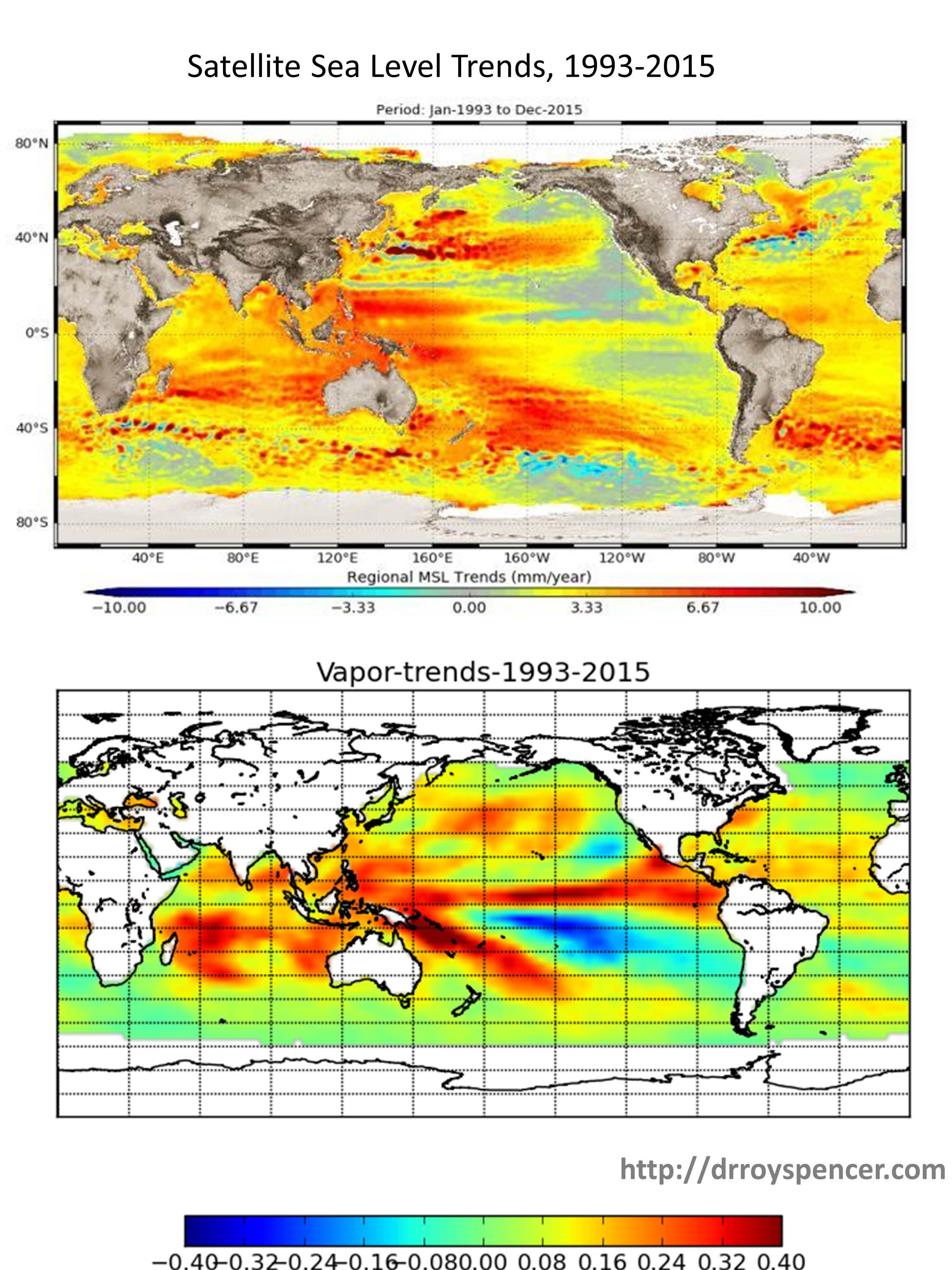 The geographic pattern of 23-years of sea level rise from satellite altimeter data looks similar to the pattern of water vapor increase (percent per decade), suggesting cross-talk between the water vapor correction and sea level retrieval.
There is considerably similarity to the patterns, which is evidence (though not conclusive) for remaining cross-talk between water vapor and the retrieval of sea level. (I would expect such a pattern if the upper plot was sea surface temperature, but not for the total, deep-layer warming of the oceans, which is what primarily drives the steric component of sea level rise).
Further evidence that something might be amiss in the altimeter retrievals of sea level is the fact that global-average sea level goes down during La Nina (when vapor amounts also go down) and rise during El Nino (when water vapor also rises). While some portion of this could be real, it seems unrealistic to me that as much as ~15 mm of globally-averaged sea level rise could occur in only 2 years going from La Nina to El Nino conditions (figure adapted from here) :
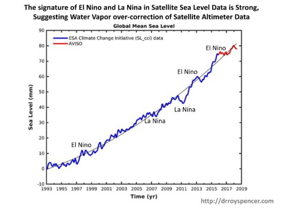
Especially since we know that increased atmospheric water vapor occurs during El Nino, and that extra water must come mostly from the ocean…yet the satellite altimeters suggest the oceans rise rather than fall during El Nino?
The altimeter-diagnosed rise during El Nino can’t be steric, either. As I recall (e.g. Fig. 3b here), the vertically integrated deep-ocean average temperature remains essentially unchanged during El Nino (warming in the top 100 m is matched by cooling in the next 200 m layer, globally-averaged), so the effect can’t be driven by thermal expansion.
Finally, I’d like to point out that the change in the shape of the vertical profile of water vapor that would cause this to happen is consistent with our finding of little to no tropical “hot-spot” in the tropical mid-troposphere: most of the increase in water vapor would be near the surface (and thus at a higher temperature), but less of an increase in vapor as you progress upward through the troposphere. (The hotspot in climate models is known to be correlated with more water vapor increase in the free-troposphere).
Again, I want to emphasize this is just something I’ve been mulling over for a few years. I don’t have the time to dig into it. But I hope someone else will look into the issue more fully and determine whether spurious trends in satellite water vapor retrievals might be causing spurious trends in altimeter-based sea level retrievals.
What is the wave length of the signal sent by the altimeters?
http://www.radartutorial.eu/19.kartei/09.space/karte004.en.html
Google is your friend (or Bing, or Duck-duck-go, if you prefer). Why are you wasting others people’s time with questions you can easily find for yourself? Really. A teacher does not do a student any favor by spoon-feeding them information they can easily go the library and find on their own. The learning process to research along the way adds much to richness of one’s education and thinking.
Really? That’s your answer to a simple question? I could educate you on some of the physics of radar and why the wavelength is important to this discussion. But never mind.
13.575 and 5.3 GHz ( Ku–, C-Band)
Assumptions aand calculations piled on top of each other there has to be documented checks and varification for each and then you would think someone would do separate analysis against other real world phenomena to verify that there aren’t other possible causes for the output especially when there is a two fold disagreement with other forms of the same measurement. Not sure there is anyone left in this world that cares about getting it right anymore. Our grandfathers must be spinning in there graves.
This is excellent work. It seems like a very plausible explanation. I believe that honest scientists would withhold any conclusions based on the satellite data until this can be fully investigated.
In any case, it is illogical to conclude any acceleration in the rate of sea level rise.
The satellite readings are inconsistent with the tide gauge readings, so at least one of the methods is providing incorrect measurements. If one does not trust the tide gauge readings for the period AFTER satellite measurements became available, then what reason is there to trust them in the period BEFORE? It is not logical to combine one series that you believe is incorrect, with a diverging series you believe is correct, and conclude that the trend has changed, when NEITHER series shows a change in the trend.
I have always wondered how they were able to measure the sea level from orbit…I know enough about the subject to know it must be complicated. What I didn’t know was the “Water Profile Adjustments”. Argh.
So I have never believed their measurements were highly accurate, but thought that at least this form of measuring was somewhat resistant to data tampering – but apparently it isn’t so. Calibrations, orbital-related adjustments, equipment degrading are all opportunities to manipulate the resulting data, but I was hopeful that there is enough separation between the engineers and the climate activists to make biased adjustments difficult. A “Water Vapor Profile” though…that is going to be entirely easy to take over and manipulate – and its obscure enough to hide. (Yeah, when it comes to data for climate, I am admittedly becoming paranoid)
I for one REALLY appreciate this posting. It has given me new information about satellite data collections I had wondered about and never understood.
I am starting to think the ONLY way we will ever be able to get at the truth is for skeptics to build a series of highly reliable temperature stations and monitor them ourselves. If we had started this effort 20 years ago, we would be in a good position to embarrass the climate crowd – or to prove to ourselves they are right. Sea level depends on so many things – like ground subsidence and sea currents- so I am not sure we could perform the same testing there.
Roy,
I am interested in to what extent any adjustments are valid. The altimetry data has been subjected to several adjustments for various reasons ever since the altimetry data showed a deceleration between 2003 and 2011.
I do not know how to evaluate the water vapor effect, but altimetry results suggesting sea levels rise during El Ninos and fall during La Ninas is consistent with the shifts in centers of precipitation and selected tide gauges. During El Nino more rain falls in the center of the Pacific, during La Ninas more rain fall over Asia and Australia where endorheic basins slow the waters return to the ocean.
A 2008 paper by Holgate analyzing just tide gauges revealed a ~20 year cycle of accelerating and decelerating sea level rise rates. There is a strong correlation with that data and California’s cycles of heavy precipitation, during which more rains falls on California during El Nino and positive PDO years.
Holgate 2008. http://landscapesandcycles.net/image/129472535_scaled_608x386.png
California precip.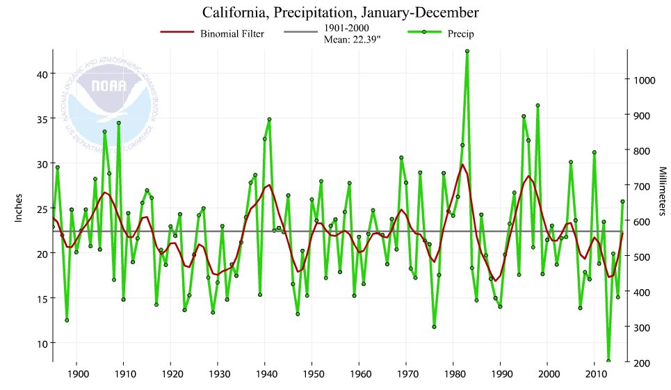
I touched on this in a recent newspaper column http://landscapesandcycles.net/sea-level-changes-part-1.html
Jim
The people responsible for preparing tide tables have known about 20-year (lunar) and longer periods for a very long time. I think that as a practical matter, rather than incorporating these long periods into their equations, they just periodically empirically re-calibrate their datums that the tides are referenced to. This also addresses the issue of land elevation changes.
Shouldn’t we only be worried about SLR along shorelines, since that is the only place it can affect Humans ? Only the tide gauges can measure along shorelines…IIRC…..
What a dog’s breakfast!
How could anyone take any of this seriously? Tide gauges, pretty simple, you can read one with your eyes. Satellite altimetry, an un-calibrated “scientific” instrument. If you cannot calibrate an instrument you do not have an instrument.
Wow, our tax dollars at work. U of Colorado should wander off and get lost…
The Jason satellite has a stated altimeter accuracy of 3.3 cm. Already Giga samples per second as it is a microwave comparator device. Not sure why the sea level guys think that reading the output a few thousand times allows them to mysteriously pretend the accuracy can be improved by the square root of N samples like random errors reading a tape measure over a known length….I’m pretty sure my instrumentation prof would have given me a failing grade on that assumption….
Just to put some numbers on this, let’s say you’re attempting to measure distance to within in 1mm through a column of humid air 10km high (that’s about the depth of the troposphere I believe?). The effective refractive index of air through that column is essentially telling you how fast light travels through there. If you have an error in the refractive index of 1×10^-7 then your distance measurement will be in error by 1mm.
I’m not sure how much RH can alter the refractive index of air but that’s the kind of numbers in play here I think.
The update should be dated March 8, not March 18.
There is radar altimeter error and the biases and corrections discussed here, there is error in determining the orbital position of the satellite in reference to a datum like WGS 84 [even with laser retroreflectors], there is datum error with respect to a geoid which itself is a model of where sea level should be [equipotential gravitational surface]. There is error in the ITRF that the Geoid is modeled on uses as an absolute frame of reference. And yet all this error has been reduced to the point that sea level can be reliably measured to a tenth of a millimeter and a change in the second derivative of sea level height detected?
Can someone explain how its done?
I think this methodology works for a spherical chicken in a vacuum. (Joke from “Big Bang Theory”.
Defining what sea level actually is, is an idealized concept.
describes the problem of defining sea level.
1)Where I live, the Pacific Plate is moving NW at between 7-11 CENTIMETERS per year. The shape of the ocean floor changes. How is this corrected for in the millimeter estimates of sea level rise?
2) Can GPS measure distances to within 1 mm?
Walt D.
https://www.gpsworld.com/gnss-systemalgorithms-methodsinnovation-accuracy-versus-precision-9889/
is an informative discussion of GPS and the differences between accuracy and precision. It looks like collecting data for hours with a DIFFERENTIAL GPS system can provide sub-millimeter accuracy. However, a single GPS cannot come close to that.
Unlike most climatologists, this guy understands metrology and the mathematics of accuracy and precision.
One of the interesting things I learned on this issue is that the sea level rise during El Nino is partly because warming in the top 100 m of ocean causes more water expansion than cooling in the next 100m causes contraction, because the coefficient of thermal expansion is temperature-dependent. (This is the global average signature in the vertical profile of ocean temperature…warming of the top 100m, cooling in the next 100 m).
Jevrejeva et al,2014 (J14) is a eustatically corrected reconstruction from tide gauge data.
The key features of J14 are a falling sea level near the end of Holocene neoglaciation phase and then a steady, secular rise of about 1.9 mm/yr since 1860 as the Earth warmed up from the Little Ice Age.
The steady rise from the Little Ice Age is punctuated by a multi-decadal quasi-periodic fluctuation (a cycle to a geologist…
If someone only looked at the data from the early 1990’s onward, they might be tempted to declare it to be an acceleration in sea level rise. However, the “acceleration” is just a function of the ~60-yr cycle.
Excuse me, but the “cycle” you talk of, as far as can see, has produced just 2.
Now would you say that that constitutes statistical significance?
Such that we know it’s causation and can be sure of it’s regular occurrence.
Over 150 years, there can only be 2 full 60-yr cycles.
Cycle 1
1870-1900 Fast
1901-1929 Slow
Cycle 2
1930-1950 Fast (~3 mm/yr)
1951-1992 Slow (~1 mm/yr)
Cycle 3
1993-Present Fast (~3 mm/yr)
1870-2010 Average ~2 mm/yr
1870-2010 clearly exhibits a pattern of SLR alternating between roughly 1 and 3 mm/yr, with an average rate of ~2 mm/yr. Each full cycle has a duration of ~60 years. The same people claiming that SLR is accelerating (Nerem et al.) actually identified a 60-yr SLR cycle.
https://agupubs.onlinelibrary.wiley.com/doi/full/10.1029/2012GL052885
SLR accelerated from 1929-1930 by ~2 mm/yr2, decelerated from 1950-1951 by ~2 mm/yr2 and accelerated from 1992-1993 by ~2 mm/yr2. There is absolutely no evidence that SLR is currently accelerating.
David Middleton (March 10, 2019 at 1:50 am )
1. “1870-2010 clearly exhibits a pattern of SLR alternating between roughly 1 and 3 mm/yr, with an average rate of ~2 mm/yr. Each full cycle has a duration of ~60 years.”
Where do you see that in the data?
Here is a chart showing us sea level data from 1880 till 2013 as provided by CSIRO, but detrended:
https://drive.google.com/file/d/14StX8gooDpkKZa4OLnmldeTBN5rayTu7/view
You immediately see
– the series’ detrended character when looking at its flat linear estimate of -0.003 mm/yr;
– its polynomial filter showing no cyclic behavior.
Try this with the AMO detrended time series, and you will immediately understand the difference.
2. “There is absolutely no evidence that SLR is currently accelerating.”
How do you manage to write that after having read the Chambers/Merryfield/Nerem paper you mention in your comment above?
I cite from their conclusions:
*
Your interpretation of this article is, to be honest, extremely strange, and probably centered around a sentence in its abstract:
Too fracking funny…

CSIRO’s fake acceleration doesn’t show up on the satellite data, upon which the bogus claim of an ongoing acceleration is based.
Right here…
Do I need to put trend lines on the pre-1930 data? The flattening from roughly 1901-1930 should be obvious to even the most disinterested casual observer.
It *is* a small fluctuation, as is the supposed acceleration and the overall trend.
Because there is no evidence of an ongoing acceleration. Nor do their conclusions mention an ongoing acceleration.
The acceleration, to the extent it was an acceleration, occurred about 25 years ago… about 30 years after the most recent deceleration.
There is an update from Dr Spencer where he has calculated the possible error if the water vapor correction were totally ignored, and that is “only” 10 %.
Firstly, I don’t know where he gets his water vapor trend (0.48 mm/decade) from. The trends of RSS and ERA5 for 1993-2018 are 0.41 and 0.53 respectively.
So RSS underestimates the trend compared to ERA5, the latest state of the art reanalysis from ECMWF, contrary to what Dr Spencer claims.
http://postmyimage.com/img2/507_WaterVaporOceans60N60S.png
Secondly, the “only” 10% error seems to be at least a magnitude too large.
According to the RSS trend the water vapor has increased by 1.07 mm in 1993-2018. If we introduce an imaginary pure water vapor layer with the density 0.6 kg/m3 (and keep the rest of the air column intact), it would become a 1.8 m thick layer.
The radar signal travels through this layer with the speed of light. If we assume that radar frequency has the same refractive index as visible light, the speed would be reduced by 1.00026 compared to that of vacuum. The sea level error would thus be (1- 1/1.00026) * 1.8 m which is about 0.5 mm.
O.5 mm is only 0.5% error, not 10% as Dr Spencer claims. My estimation may be simplified, so please correct me if I’m wrong..
Olof R
You said, “… I don’t know where he gets his water vapor trend (0.48 mm/decade) from. The trends of RSS and ERA5 for 1993-2018 are 0.41 and 0.53 respectively.”
The average of 0.41 and 0.53 is 0.47. That might be a clue.
You further remarked, “If we assume that radar frequency has the same refractive index as visible light, …” I would be very surprised if that were the case. In attempting to correlate the refractive index of minerals, as measured with visible light, with their dielectric constants at RF frequencies and DC, I have found no correlation. Most materials have a strong dispersion of refractive index even for visible light, let alone with EM radiation orders of magnitude longer wavelength. Things are further complicated by the fact that, strictly speaking, ALL refractive indexes are complex and the inverse relationship is a first-order approximation that is only valid for ‘transparent’ materials. If there is strong absorption at any particular wavelength, then that indicates that the extinction coefficient in non-negligible. That is, the complex RI has to be used in calculations for that wavelength.
No, I don’t think Dr Spencer uses the ERA5 dataset, he has never mentioned it. Possibly it is ERA-interim which has a trend of 0.46 kg/m2/decade.
I dont think the refractive index of radar wavelengths is very different from that of visible light.
The explanation is probably that the radar measurements are not only done vertically. They also use skewed angels to cover larger areas of the ocean. In the latter case the increased water vapor content near the surface will bend away the radar signals, such that they travel a longer distance, which requires much larger correction than that of strictly vertical measurements.
Here is a paper on the wet troposphere corrections used in the AVISO altimetry:
https://www.sciencedirect.com/science/article/pii/S003442571530081X
Quite complex, but at least I can say that they use Era-interim vapor data for corrections.
Since the brand new ERA5 total vapor has a slightly larger trend, I guess that the AVISO sea levels will be adjusted up slightly in the near future..
Thanks Olof, you raised interesting points here I would never manage to discover.
Dave Middleton (March 10, 2019 at 10:50 pm, March 10, 2019 at 10:17 pm)
1. “… Nor do their conclusions mention an ongoing acceleration.”
Here you are right. I forgot to insert a paragraph in my last comment. Good grief!
2. “The acceleration, to the extent it was an acceleration, occurred about 25 years ago? about 30 years after the most recent deceleration.”
Here is the plot of CSIRO’s five-year running means, from 1883 till 2008:
https://drive.google.com/file/d/1n3gyDRgvK5kbYkA1SymZfSMW5Cpw0tc4/view
Source:
http://www.cmar.csiro.au/sealevel/GMSL_SG_2011_up.html
I suppose you understand that if there was no acceleration, the running trend plot would look like a straight line, wouldn’t it?
3. “CSIRO’s fake acceleration doesn’t show up on the satellite data, upon which the bogus claim of an ongoing acceleration is based.”
So? How then do you explain the sat altimetry trend differences for two periods:
1993-2013: 2.89 mm/yr
1993-2017: 3.16 mm/yr
It is nearly the same difference as that between the gauge/altimetry trend difference for 1993-2013.
Here are the trends for different starting dates till 2017:
1993-2017: 3.160 ± 0.018
1998-2017: 3.339 ± 0.025
2003-2017: 3.463 ± 0.039
2008-2017: 4.256 ± 0.064
2013-2017: 4.641 ± 0.160
Yes, Dave Middleton: so it is, wether you like it or not.
Source:
http://sealevel.colorado.edu/files/2018_rel1/sl_ns_global.txt
*
If you don’t believe me, feel free to download all the data and process it by your own.
*
Before somebody describes the work of others as „fake“, shouldn’t s/he provide for an own scientific contradiction? This would be my way, assuming I am able to. If I am not, I prefer to remain silent.
For Patrick Geryl (March 8, 2019 at 10:32 pm)
Comments closed there, many thanks for the F10.7 info.