My links to comments did not survive, so I added more information to help find the original comments in the original post.
The following comments are from Dr. Ronan Connolly and Dr. Michael Connolly. They are in answer to comments made on my review (see here) of their atmospheric physics papers. I’ve promoted the comments to a post because they are very enlightening and should be of general interest to our readers.
Dr. Michael Connolly’s comment below is in response to Dave (August 22, 2017 7:38AM and August 25, 2017 1:54PM).
In part, Dave says: “Two requests have already been made as to how this tetramer runs contrary to the law of mass action. A law that is best derived by a combination of the Gibbs free energy values for the reacting species. For the tetramer formation it is p (O8) = K p (O2)^4.”
The response also mentions a comment by Nick Stokes (August 22, 2017 10:34AM).
In part Nick says: “It seems that the data they are actually working from is measured pressure and temperature. So, they define molar density D = P/RT; the identification of that as density comes from the ideal gas law (which is ideal…).
So then, in Figs 4/5, they plot D against P. Is the slope of this not just 1/RT? And the “regime changes” just changes in T?”
Dr. Michael Connolly (I’ve edited this a bit for clarity) August 26, 2017 3:18AM:
I would like to thank Andy May for doing this blog post and all the participants for their interesting contributions. I am sorry that due to time constraints I could not contribute to the discussions as they were taking place. However, I have read all the contributions and I think the following observations might resolve many of the difficulties, but will also raise more problems (at least they do for me).
In paper 1 we reported that the slope of molar density (D = P/RT) plotted against pressure (P) is greater in the Tropopause – Stratosphere than in the Troposphere for all 13 million Radiosondes that we analysed.
Look at the video for Valencia that Ronan posted earlier in this thread (middle panel).
Link to video here.
This is a head scratcher, because according to the current theories of atmospheric behaviour, it should be the other way around (i.e. the slope should be smaller in the Tropopause-Stratosphere than in the Troposphere). As has been pointed out the slope should be 1/RT.
In the Troposphere T decreases with pressure. To increase the slope in the Tropopause –Stratosphere, T would have to decrease at a greater rate. (The slope is the reciprocal of T i.e. increasing T decreases the slope and decreasing T increases the slope). But the temperature does not decrease at a greater rate in the Tropopause, it stops decreasing all together, and in the Stratosphere it actually increases (See the top panel of the YouTube video Ronan posted).
The current explanation of the temperature profile in the Tropopause- Stratosphere region is that it is caused by UV heating of this region. But heating this region should decrease the slope of D versus P, which is the exact opposite of what happens. Therefore, a different explanation is required.
In paper 2 we suggest that a phase transformation from monomers to multimers, in the Tropopause – Stratosphere, if it took place, could explain the behaviour. An increase in the average molecular weight of the atmospheric gases in this region, would explain an increase in the slope of D versus P plot.
But is such a phase transition thermodynamically feasible? If not, then another explanation is required, and it may well be that another explanation will be found. However, now the only explanation we have come up with is the multimer hypothesis, and this is not without its own difficulties. For a gas phase reaction of the form nX2 ↔ (X2)n the value of the equilibrium constant (which is determined from the partial pressures of the reactants and products) can be used to calculate the direction of the reaction if the change in Gibbs free energy for the reaction is known.
For a closed system, it is sometimes possible to determine the value of the change in Gibbs free energy by experimentally changing the values of the state variables. However, in an open system this is not the case. In a closed system, the change in Gibbs free energy is a tradeoff between the heat of formation of the products and the change in heat capacity caused by changes in entropy(s) due to the reaction. However, in an open system, such as the atmosphere, where the value changes in the various components of Gibbs free energy (i.e. the heats of formation and changes in heat capacity of the reaction) are unknown; Gibbs is of no value.
This is very unsatisfactory, in section 2 of paper 2 we have attempted some heavily caveated “work arounds” but more experimental work is needed before the multimer hypothesis can be confirmed or rejected.
With respect to paper 3, in our day job we do a lot of work with heat pumps and heat exchangers and I have been awarded patents for novel designs of the same. For years a lot of our designs did not perform as theory predicted. It was only when we realized that we had had been neglecting through-mass mechanical energy transmission in fluids (as had everyone else) and that by taking this into account, that we could reconcile theory and performance. Steven Wilde (see here) in this thread said that there was no need to invent through-mass (non-acoustic) mechanical transmission which we call ‘pervection’. Well we did not invent it, nature did that all on its own. All we did was name it, measure it and now use it.
Dr. Ronan Connolly (also edited a bit) August 23, 2017 3:55PM:
Further research on our multimerization theory since our 2014 papers
Since those papers in 2014, we have been continuing our research into this phase change as well as into our multimerization theory. We have also been discussing our analysis with several prominent atmospheric physicists and chemists, and their comments have been generally encouraging.
Some commenters above (see Dave’s comment here) have wondered if our multimer theory could be tested under laboratory conditions. Yes, indeed, last year we carried out some preliminary experiments to reproduce tropopause/stratosphere temperatures and pressures in the laboratory. The results were suggestive of multimer formation, but the experiments were quite expensive and time consuming, and we don’t think we have collected enough data yet (in our opinion) to publish these findings. We do plan on completing these experiments at a later stage, but bear in mind we’re carrying out all this research in our spare time and at our own expense!
Still, in case you’re interested, we carried out a series of 8 experiments in which we evacuated dry air in a glass container to pressures down to about 20,000 Pa (200 mbar) and lowered the temperature using dry ice. We recorded the temperature and pressure of the air continuously throughout each experiment, and from these measurements we could also calculate the molar densities. Below about 200K we found that the molar density started to drop by a few percent, which is what we would expect from multimer formation. We also carried out several experiments using oxygen instead of air and found that the drop in molar density was about 5 times greater. Since air is only about 1/5 oxygen, this suggests that, if our multimer theory is correct, then oxygen is the main gas that is forming multimers.
We have also been in discussion with several groups about the possibility of analysing these experiments spectroscopically. In particular, we are looking at testing for changes in magnetism (monomeric oxygen is paramagnetic, but it is plausible that multimers could be diamagnetic), as well as testing for microwave emissions. [It has been reported by Spencer and Christy (1990) that the Tropopause is a source of unusual microwave emissions.]
Nick Stokes and Dave on plotting P vs. P/RT
When we first started analysing the weather balloon data, we expected it would be exactly how Nick Stokes and Dave described. We would have expected a plot of molar density (D=P/RT) vs. P to yield a simple linear plot of slope 1/RT. But, instead, the data consistently shows a bi-linear behaviour. We analysed over 13 million weather balloons (taken from over 1,000 stations with some data going back to the 1950s), and this bi-linear phenomenon occurred for all the balloons.
I showed this video in my reply yesterday, but in case anyone missed it, here are the plots for one year’s data for the Valentia Observatory station in Ireland. The D vs P plots are shown in the middle panels. For comparison, the top panels show the standard T vs P equivalents:
In all cases, the circular dots represent the experimental data. The two lines in the middle panels illustrate the change in slope. As Nick pointed out, this slope should in theory be constant (1/RT) for the entire plot. But, as Andy pointed out, it’s not.
I realise that many in the climate science field argue that if the data doesn’t match the theory, there must be something wrong with the data. However, we’re a bit more old-fashioned, so when we find an apparent conflict between the theory and the data, we try to consider the possibility that the theory might be wrong.
On our atmospheric temperature profile fits
In Nick Stokes’ August 22, 2017 at 3:23 pm comment, he criticises our analysis in Section 3.2 of Paper 1.
For those who haven’t read this section yet, we point out there that, for a given balloon, after obtaining the linear fits for each of the two linear regions, you can then use the slopes and intercepts to estimate the atmospheric temperature profile. When you compare these estimates to the original observations, the fits are remarkably good (in our opinion), i.e., the residuals are very small. Andy has shown some of these plots in his post. We think it is striking that the entire atmospheric temperature profile can be described so well merely in terms of the fitting parameters of two (or sometimes three) straight line fits. To us, this suggests that using D vs. P plots could be a very powerful tool for meteorologists.
Because triplet oxygen has two unpaired electrons?
Probably so. Found this patent which describes a process to induce the polymerisation of oxygen using high pressure, high temperature and UV light. The first two factors obviously are absent in the higher atmosphere layers, but UV is not.
Quite a bit out of range of my element here… but have there been any experiments to determine the effect of the solar / planetary magnetic plasma conduits on upper atmosphere chemistry? It seems that this phenomenon might provide another factor in the energy and charged particle / reaction-driver / catalyst mix for multimers in the upper atmosphere. Even mall amounts of plasma would be more powerful than even UV light in sustaing radical-fostered reactions and combinations.
IMO the mass of the atmosphere, regardless of its chemical composition, does have an effect on planetary surface temperature.
However, I have experienced the greenhouse effect on nights with high humidity. Water vapor does indeed keep the air warmer than if it were dry.
But going from three molecules of CO2 per 10,000 dry air molecules, as a century ago, to four such molecules today, is a far cry from the difference between four H2O molecules and 400, as is the case in the moist tropics.
Earth has provided us with many experiments in the GHE. Just compare nighttime lows of locations at the same latitude, elevation and daytime high temperatures but with low and high humidity.
The GHE of another molecule of CO2 however is negligible at best, and probably not measurable. The only places at which the effect might be detectable would be where water vapor is very low, as over the polar deserts. Yet the South Pole has shown no warming since record keeping began there.
I agree. It has always surprised me that I’ve not read of any attempts to measure the CO2 GHE in Antarctica. After all, they have a CO2 measuring station at Jubany station. You would think if it can be measured at all, it could be measured there. In winter time the water vapor content must be essentially zero. They have measurements back to 1994, it would seem possible to design a way to detect the effect, if any.
The funding powers that be might be afraid of the result. Under Trump, maybe US government scientists at the Pole station will feel free to analyze the data.
Even if not zero, H2O content might at best equal CO2.
Hasn’t been done in Antarctica, but it has been done.
https://wattsupwiththat.com/2015/02/25/almost-30-years-after-hansens-1988-alarm-on-global-warming-a-claim-of-confirmation-on-co2-forcing/
Note that they got only 0.2 w/m2 per decade. No wonder we can’t measure the signal, its almost zero!
davidmhoffer, thanks. Do you have a link to actual paper? I didn’t see one in the post.
Andy,
This is the only link I have:
http://www.nature.com/nature/journal/v519/n7543/full/nature14240.html?foxtrotcallback=true
David,
Thanks! Forgot about that post and paper.
I like how that abstract is carefully worded.
That Nature study claims to have measured changes in radiation, and to have used “ancillary measurements” and “highly corroborated calculations” to correct for distorting influences, all within an error of +/- 0.06 W/m^2. That is something like 0.02% of the total irradiation. I do not believe this.
davidmhoffer and Michael Palmer, If their study did detect a clear sky CO2 effect in Oklahoma and Alaska of 0.2 W/m2 +-0.07 W/m2, it is very small. They have to assume massive (factor of 3 or more) positive feedbacks to the additional CO2, which is in serious doubt. I grant the possibility they are correct in their assessment, but I don’t think this small amount says anything about what the Connolly’s found. Thanks for the link.
I would wager that the Russians would be willing to make the observations, as they are not wedded to the CAGW scenario. I believe they maintain suitable sites in the East Antarctic highlands, e.g. Vostok.
When looking at the Feldman et al paper one also needs to look at Gero/Turner 2012. They look at the total change in downwelling IR and found either no change or it actually decreased during the same period where Feldman found an increase in CO2 IR energy.
This could be construed as evidence of negative feedback as proposed by Bill Gray.
As for Antarctica, there was a paper where they looked at the GHE and found that in many places it was actually negative.
http://onlinelibrary.wiley.com/doi/10.1002/2015GL066749/full
Here’s Feldman 2015:
http://sci-hub.bz/10.1038/nature14240
Atmospheric physicist Will Happer has found evidence that the warming effect of CO2 is commonly overestimated by about 40%, due to the use of Voigt profiles to model the spectral lines, which calculates overly broad far fringes of the lines. He discussed it in this UNC Physics Colloquium:
http://www.sealevel.info/Happer_UNC_2014-09-08/
There’s this:
Climate Change 2007: Working Group I: The Physical Science Basis
8.6.2.3 What Explains the Current Spread in Models’ Climate Sensitivity Estimates?
In the idealised situation that the climate response to a doubling of atmospheric CO2 consisted of a uniform temperature change only, with no feedbacks operating (but allowing for the enhanced radiative cooling resulting from the temperature increase), the global warming from GCMs would be around 1.2°C (Hansen et al., 1984; Bony et al., 2006).
In theory increasing CO2 should cause some warming but whether it actually does or not – as you point out with the South Pole example – is another matter.
If CO2 is responsible for .2W/of forcing in a location of nearly zero absolute humidity, what portion of that forcing would be taken up by latent heat change on the 71% of the Earth that is ocean and the land area that has significant moisture levels. Additionally, the Antarctic is so dry it probably tends not to have a lot of cloud cover so that forcing is relative to that as well.
Take the .2W, subtract cloud reflective averages, factor the latent heat changes and my guess is we are within the margin of error for the overall effect to be essentially zero when actual temperatures are taken on a worldwide basis.
Some questions:
Do we have measurements of the greenhouse effect of certain quantities of H2O / water vapour in the atmosphere?
And if so, what do they show?
What is the total greenhouse effect of H2O / water vapour at different temperature levels?
Wim, Murray Salby provides an estimate on page 241 of his textbook on Atmospheric Physics (2012 edition). He says water vapor accounts for 80-90% of overall cooling. It amounts to 2K/day in long wave cooling in the troposphere. He says carbon dioxide and ozone dominate in the stratosphere. However, he is only talking about radiative longwave IR cooling. This does not include the effects of convection, pervection or latent heat storage. The latter mechanisms cannot get the radiation into space, but they can increase the speed of cooling, which is really the issue.
Warming is mostly short wave absorption by the oceans, but some short wave absorbtion takes place in the atmosphere by water and ozone.
I think Wim was asking about actual measurements. I’ve been following this sorry field for many years now, and have yet to see lab measurements of back radiation from, for example, 280ppm CO2 on a background of water vapor from zero to 40,000ppm, compared with 408ppm CO2 on the same background. Equipment to accomplish this would cost peanuts on a scale of things. You might even be able to add in convection too for another couple of hundred thousand.
If you go back to the original Modtran paper it involves models.
So why not? Do I need to ask?
philincalifornia August 26, 2017 at 4:15 pm: “I think Wim was asking about actual measurements.”
WR: Completely correct. I know estimations for the share of H2O in backward radiation / greenhouse effect.
In this paper Gavin Schmidt estimates that the total single factor addition of water vapour and clouds to net LW absorbed together is 80.9%.
Elsewhere I read estimations of 90-95% and more. Therefore my question: “Do we have [omitted: actual] measurements of the greenhouse effect of certain quantities of H2O / water vapour in the atmosphere?
It must be very interesting to do measurements at different temperature levels – all other things remaining the same, which is not in reality. See: afonzarelli August 26, 2017 at 5:03 pm: “think also of the claim that’s been made for co2’s affect on temperature coming out of a glacial. (the claim is that about a third of the .4-.5C warming is caused by the half way to doubling of co2) Changes in water vapor alone would dwarf the contribution of co2. So how is it possible that co2 could play anything but a minor role in warming?”
Wim Röst August 26, 2017 at 11:02 pm – forgotten links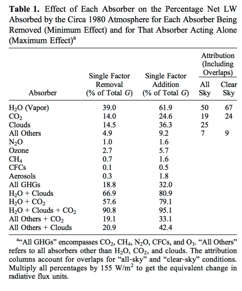 :large
I forgot the links to table 1 of Gavin Schmidt and the paper:
Table:
Source:
https://pubs.giss.nasa.gov/docs/2010/2010_Schmidt_sc05400j.pdf
Gloateus August 26, 2017 at 7:23 pm “a high share of my attempts never appear”.
WR: Possibly you use key combinations the system does not accept. I recently tried to produce a smiliey at the end of a comment using the keys of my keyboard. The comment disappeared. The only unusual thing in my comment was the ‘smiley by keys’.
I trick I sometimes use is: writing the comment in Word and copy it to the “reply” possibility. Even when it should disappear, I still would have the original.
Wim, my “.4-.5C” should read “4-5C” (i’ve got a knack for ruining my best comments… ☺)
Wim, i got the idea for my comment from a geologist who chimes in over at dr spencer’s blog who goes by the name of “aaron s”. (very nice fellow…) i really thinks it’s time to blow the horn, so to speak, on his idea. Should be interesting for me personally, because i really don’t have much of an idea of precisely how the energy budget goes from ice age to interglacial. Never have come across any literature on it (so it should be interesting to see if anyone else has)…
afonzarelli August 27, 2017 at 12:44 am:
“i really don’t have much of an idea of precisely how the energy budget goes from ice age to interglacial”
and:
“Wim, i got the idea for my comment from a geologist who chimes in over at dr spencer’s blog who goes by the name of “aaron s”.”
WR: Afonzarelli, my guess that it is not the energy budget that is the cause of the change from glacial to interglacial, but a diminished cooling by the cold deep oceans (by less wind and so: less upwelling of cold deep water into the warm surface layer). The energy budget will change, but as a result of ‘ocean moves’.
Do you know an excerpt of the ideas of Aaron S? Could be interesting.
Wim Röst August 26, 2017 at 11:02 pm
Exactly Wim.
Plus, I’m pretty certain that equipment could be designed that would handle pressure/Doppler line-broadening effects and would show that climate sensitivity to anthropogenic CO2 in humid air is zero, and we already know it’s zero in Antarctica where there’s low to zero WV.
The question is, when will the prosperity-destroying phonies and mental masturbators give up and tell the lying conniving politicians the truth ??
Gloat, think also of the claim that’s been made for co2’s affect on temperature coming out of a glacial. (the claim is that about a third of the .4-.5C warming is caused by the half way to doubling of co2) Changes in water vapor alone would dwarf the contribution of co2. So how is it possible that co2 could play anything but a minor role in warming?
Another reply gone missing.
I won’t try to recreate it. Too long.
Gloateus, I just checked the comment queue, there is nothing there. I don’t know what happened to your comment.
Andy,
The same thing happens to me every day, including twice today. Even when I save and try to repost, a high share of my attempts never appear. Some do show up later, but most don’t.
I’m at the point that I feel like giving up on commenting here at all.
Maybe word press is doing some stealth sabotaging of this site. (☺) Anthony mentioned before his hiatus that he was thinking about getting new software upon his return. Let’s hope he hasn’t forgotten…
“.4-.5C” should read “4-5C”
Andy, no response regarding to how multimers help form Ozone with less energy? Fig. 6 still shows the breaking of the diatomic oxygen bonds.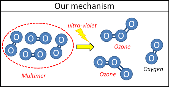
I know and perhaps the Connolly’s will chip in here. I can only point you to their discussion in paper 2, section 3.3, starts at line 1423. The key bit of the explanation is in lines 1548-1575. It seems to conclude that their mechanism is faster and is a one-step process. The Chapman process is a two-step, second order reaction. I hope that helps.
If “less energy” simply means “less free energy”, then the argument would be that multimeric oxygen has lower entropy than regular free O2.
Hmm. I’ve had at least 1 bottle of wine in the last few hours but this does not seem to make sense. How in the hell can a multimer have more entropy than free O2 molecules? dg = dH – TdS so there is also an enthalpy term to consider but in my view a multimer can never have more entropy than free molecules. Unless the O2 molecules associate with water and the multimer frees up water (as in the hydrophobic effect).
But O2 is 18-20% of the atmosphere, much more than water vapor so that seems unlikely.
In my reply, I was assuming 1) that the multimers are not covalently bonded, 2) that they exist at equilibrium with the O2 monomers, 3) that they are higher in G than the monomers, due to the loss of entropy. If 3) is the case, then the additional step up in G to reach ozone is reduced. Does that make sense now? If not, keep adding more wine 😉
Hi Duncan
Sorry it has take so long to reply to your valid question.
The Chapman mechanism proposes
1) the UV light dissociates an oxygen molecule into two oxygen radicals
2) each of these radicals then combine with an oxygen molecule to form ozone in an excited state
3) These excited ozone molecules must then collide with a third particle so that they can transfer energy, in the collision process, to this third particle, before they can dissociate again.
If multimers exist (and it is still conjecture at this stage), then the reason why we think that ozone could be formed with lower energy UV (and this is also conjecture) is that multimers could allow the formation of ozone in the ground state, in the same way that other catalytic processes work.
In other words, the extra energy carried off by the third particle in the Chapman mechanism would not be required.
What isn’t conjecture is the remarkable similarity between the concentration of ozone and the pressure of the phase change boundary, which can be seen in figure 13 in paper 2. The Chapman mechanism does not offer an explanation for this similarity.
Ideal Gas Law:
PV = nRT.
PV/nRT = Z = compressibility factor = 1 for an ideal gas and ≠ (not equal to) 1 for a real gas.
Interesting things can happen when V = 1 (i.e. forced or constrained volume).
What interesting things?
Andy: I suspect the Connelly’s need to review their math:
D = P/RT
dD/dP = 1/RT + (1/R)*[d(1/T))/dP]
If T were a constant, the second term in the chain rule would be zero. If T could be expressed as a function of P, we could take the derivative mathematically. However T varies independently from P because not all changes in temperature are caused by changes in pressure. So dT/dP exists as a quantity, but we don’t have an analytical expression for it. If symbol manipulation skills haven’t totally deteriorated:
dD/dP = 1/RT – (1/RT^2)*(dT/dP)
So the simplistic idea the slope should vary with 1/RT is incorrect. And it is most incorrect where T is changing fastest with respect to pressure/altitude. (:))
Frank, I’d like to see what Ronan or Michael have to say, but you may be correct. In any case, their analysis of the weather balloon data does show that T is not a simple function of P. There is more at work here, especially in the tropopause and above it. And then, we need to explain why T appears to be a simple function of P between the top of the boundary layer and the tropopause. Working out the math is more satisfying after you know what is going on. Do you think your analysis is inconsistent with the upper troposphere being in thermodynamic equilibrium?
Thanks for the reply. In tropical troposphere and elsewhere, convection and adiabatic expansion/contraction control the temperature change with altitude. In adiabatic expansion, IIRC, P^(1-g)*T^g = constant, where g = gamma = Cp/Cv = 5/3 for diatomic gases. In this part of the atmosphere, we do have an analytical expression for dP/dT. T = K’*P^(2/5)? dT/dP = (2K’/5)P^(-3/5)? Maybe this will clear up some of the mystery.
Frank, it depends if they’re calculating the derivative of D with respect to P. It seems they’re just doing a simple ratio D/P in accordance with the ideal gas law. In that case, if air in the tropopause behaves like an ideal gas, they can just replace the ratio D/P with the inverse of temperature T. Just measure T and you get the ratio.
However, if the air deviates from the ideal gas law because T is low at -50 C in the tropopause, they have to use the Van Der Waals equation:
(P + n^2 a/V^2) (V – n b) = n R T
where for nitrogen a = 1.39 and b = 0.03913
for oxygen a = 1.36 and b = 0.03183
Dr. Strangelove wrote: “Frank, it depends if they’re calculating the derivative of D with respect to P.”
If you look at the video in one of Connelly’s comments to the earlier post, they are plotting density vs pressure and complaining that the result is not a straight line. I THINK I have a perfectly sensible explanation for why the line is not linear: Textbook atmospheric physics doesn’t predict a linear relationship. However Connelly don’t have to have shown conventional atmospheric physics and then clearly defined where they think new phenomena are needed to better explain what we observe. Until they do so, it is impossible to properly evaluate their work or my comment. (These problems are typical of “blog science” and are rarely fixed.)
https://wattsupwiththat.com/2017/08/22/review-and-summary-of-three-important-atmospheric-physics-papers/comment-page-1/#comment-2587932
Thanks for looking up the correction factors for non-ideal behavior of nitrogen and oxygen gas. They are also an important part of what “textbook” knowledge tells us we should be observing. I still need the correct units to calculate how bid the correction factor is near the surface and in the stratosphere.
The ideal gas law is an equation of state. It’s an algebraic equation. Differentiating it will convert it to a differential equation. Differential equations are equations of change. They are not the same. Equations of state just say what State A and State B are. They don’t say how the system went from A to B. That’s described by equations of change. They won’t give the same answer. It’s just math, not a fundamental change in physical laws.
Correction:
dD/dP = 1/RT + (P/R)*[d(1/T))/dP]
dD/dP = 1/RT – (P/RT^2)*(dT/dP)
P^(1-g)*T^g = constant is only true for dry air. One needs to correct for water vapor.
Could there be unknown chemical species (dimers or multimers of the main gases) in the upper atmosphere?
Almost certainly not if they are created by simple collisions. Le Chatlier’s principle and reaction kinetics tell us that equilibrium shifts towards dimers and multimers at higher pressure. Furthermore accurate radiative transfer calculations require laboratory experiments at a wide variety of temperature and pressures to accurately characterize line broadening by collision/pressure and by Doppler shift/temperature. So these gases have been studied at under the conditions found in the stratosphere. (The experimental set up in one paper I read involve a laboratory apparatus that used mirrors to create a 200 m (0.2 km) path length for measuring the absorption spectrum a very low pressure.) If unexpected absorption lines were present, they should have been observed. And experimenters are characterizing minor isotopic species such as CO2 with C13 or O18 or both. So these spectra are studied very closely.
These IR spectroscopy experiments may not involve UV radiation, so novel species could be created photochemically. However, ozone depletion was a very hot research area in the 1980’s and lots of experiments were done simulating stratospheric conditions with UV. And they were trying to identify minor species like chlorine atoms, ClO, ClONO2, etc. If any unexpected dimerization occurred, it could have been caught. Knowledge of all of the species present in the stratosphere was extremely important to a full understanding of ozone depletion. The chemistry of the stratosphere is a well studied area.
Thanks for your effort in trying to resolve this. You have got my interest in trying to resolve this. I have had extensive experience using vacuum systems and cryostats on the laboratory scale and industrial and so should be able to offer some practical insights into the experimentation. For example in the dim and distant past we used to use the rather simple and in expensive molecular weight bulb to ascertain the gas densities directly from measurement as opposed to using the gas law. Also what type of pressure gauge were you using? How did you control and measure the temperature? Is it possible to issue data from a number of radiosonde in table form with dates, times showing actual pressure, both barometers, temperature and humidity so that we can independently go through these calculations?
Have you contacted the climate science section of the University of Manchester, they were most helpful to me the last time I contacted them.
As to the tetramer, thermodynamic data for oxygen is published in JANAF, which is available on line.
The tetramer is not included. However you could use the Law of Mass Action equation without actual deltaG values simply by applying the pressure relationships at the temperature you indicate that the tetramer occurs and the effect of changing the pressure will have on the tetramer concentration or partial pressure. Keeping the system isothermal will avoid the need to know thermodynamic parameters since
deltaG = -RTlnK. There should be very little dependance of detaG on presure. If needed then pressure will affect G from G = H + ST, and H= U +PV should sort it out.
I will be very interested in how we get on
Thanking you in advance
Thanks Dave, this is definitely a question for Michael. I’m sure he will get back to you. He loves this stuff.
Hi Dave
As it happens In 2015 I was having Lunch in the canteen at Manchester University where I happened to sit beside Geraint Vaughan We got talking and our mutual interest in climate came up. Professor Vaughan kindly invited me back to his office where I was able to download and discuss the Valencia video with him.
Unfortunately there is only so much you can discuss in an hour, I had to catch a train to Sheffield and he had another appointment. However I did find the discussion useful and enjoyable.
Like you I have extensive experience in working with high vacuum systems, carrying out spectroscopic studies on sub monolayer adsorption on surfaces, and have published several papers on the topic.
I have also spent several years teaching differential calculus and thermodynamics. So it goes without saying that I spent a long time manipulating the equation of state for an ideal gas, in an effort to explain (without success) the bilinear behaviour of the molar density plots. The problem always comes down to how does “dT/dP” behave for a radiosonde. In thermodynamics, differential calculus is useful for manipulating an equation of state in order to determine the behaviour of a system. Unfortunately if the equation of state of the system changes, in some unknown way, for some unknown reason then one has to resort to other approaches. Fortunately the experimental data from the radiosondes tells us that dD/dP is linear with a slope of a1in region 1 and a slope of a2 in region 2. In the appendix to paper 1 using the definition of the bulk modulus for a gas we were able to derive a theoretical value for the slope.
I have to go to work now but I will get back to this later.
So you have not given an answer as to how this oxygen multimer appears to disobey the law of mass action. The value of deltaG is irrelevant, it is the relationship between the partial pressure of the monomer to the fourth power to that of the multimer to the power 1 that you are not addressing.
Dave
I was hoping that on consideration you could work it out for yourself.
The law of mass action is now only of historical interest and was use to try and predict the rate of a reaction, but not the direction. Thanks to the work of Gibbs, it is now known that if you know the change in Gibbs free energy for the reaction, you can determine the direction of the reaction by the whether the change is positive or negative. The rates of reactions are the subject of the field of chemical kinetics which is too large to explain in a blog post. If you wanted to form a mist of small water droplets of say 1000 molecules per droplet the denominator would be raised to the 1000 power. It may not rain in your neck of the woods, but Andy May will tell you a different story today.
Micheal wrote: “The problem always comes down to how does “dT/dP” behave for a radiosonde.”
In general, heat transfer by SWR and LWR means that T varies independently from P. There is no simple theory that can predict dT/dP for the entire atmosphere – except for the region where moist adiabatic expansion/contraction controls the relationship between T and P. That region is the troposphere in the tropics and warmer seasons in the temperate zone. In the figure below, those regions that have the same moist potential temperature from the near the surface to the top of the troposphere.
https://scienceofdoom.com/2012/02/12/potential-temperature/
Heat transfer solely by radiative transfer in the lower atmosphere would create an equilibrium lapse rate that increased exponentially as one approaches the surface (with optical density) – a lapse rate that is unstable to buoyancy-driven convection. Radiative transfer calculations suggest that surface temperature would be about 350 K from radiative transfer without convection.
The gradual change as you move poleward in this figure (which represent annual averages), shows that radiation becomes more important and convection (constant moist potential temperature) less important.
What would the temperature of earth’s atmosphere be, if it had the same pressure but it consisted only of monatomic inert gases (He, Ne, Ar, Kr). How would the addition of CO2 affect the result?
Walter, I have no idea. But, if the Earth had no water and no oceans it would be very different.
I underspecified. I meant to specify that the oceans were the same.
Walter Sobchak, See my comment to Wim and Frank below. I have a problem with black or gray body calculations of what the temperature of the Earth would be under unrealistic conditions like helium atmosphere, no water vapor, and oceans covering the Earth. Or Earth with the same albedo, but no GHG’s, etc. These conditions can never exist and they treat the oceans as an afterthought. As Wim Rost has written, I suspect the oceans drive long-term climate change, they have almost all of the heat capacity and receive almost all of the short wave radiation from the sun, either directly or through river discharge. I’m not sure (and no one is) that the atmosphere has much of an effect at all and certainly the GHGs have little effect, other than radiating IR away once energy makes its way from the surface (mostly the oceans) to a high enough altitude.
Walter, this is a question I’ve long struggled with. The greenhouse effect is used to explain all of the difference between the average brightness temperature of earth and the average surface temperature. It is said that the earth would be frozen if not for the greenhouse effect. But this seems incorrect. Sunlight warms the surface so air in contact with the surface is warmed by conduction. This warmed air rises so that more air is brought in contact with the surface. Rising air cools adiabatically and by radiating some of it’s heat to space. This mechanism does not change if there are no active greenhouse gases in the atmosphere. Air near the surface would still be warmer than air at altitude and, given the intensity of sunlight, it seems to me that the average surface temperature would still be well above freezing; maybe not measurably different than the current average temperature.
Gloateus mentioned that he has experienced the greenhouse effect—due to water vapor—because in the tropics the night stayed warm while the dry desert cools off quickly after sundown. That could be due to the greenhouse effect but it could also be due to the fact that the humid air has much higher heat content than the dry air, so it takes longer for it to cool off. For example, a tropical evening at 80 °F with 80% relative humidity has a total heat content of 38 Btu/lb, while a desert evening also at 80 °F but with just 10% relative humidity has only 21 Btu/lb. The tropical air has nearly twice the total heat content of the desert air.
The above example also demonstrates why temperature is a poor proxy for atmospheric heat content.
The oceans contain 99.9% of the heat capacity of the Earth’s surface. Water vapor can store latent heat for a long time in clouds and open air. Without water and water vapor, the Earth may be like the Moon and very hot in the daytime and very cold at night. I doubt an inert atmosphere, without water, would do much. The Earth’s rocky surface wouldn’t store much energy for very long, neither would the atmosphere. By morning, it would probably radiate it all away to space.
Thomas: Perhaps I can straighten out some misunderstandings.
“Sunlight warms the surface so air in contact with the surface is warmed by conduction. This warmed air rises so that more air is brought in contact with the surface.”
When air rises and expands under reduced pressure, it cools. If the “risen parcel of air” is now cooler than the surrounding air, it immediately sinks back to where it came from. Large scale “buoyancy- driven” convection requires that the temperature drop with altitude enough so that “risen parcel of air” is still warmer than the air it has penetrated from below. That means the decrease in temperature needs to be less than the moist adiabatic lapse rate – which is somewhere between 4.9 and 9.8 degC/km, depending on how much water the air contains.
The presence of GHGs in the atmosphere creates a temperature gradient in the atmosphere. That temperature gradient is linear with optical density. If the exponentially increasing density of the atmosphere as one approaches the surface, an atmosphere in radiative equilibrium will have a temperature that rises exponentially as one moves into denser air near the surface. Some calculations suggest that the Earth without convection and with radiative equilibrium would have a surface temperature of 340-350 K. That temperature gradient would be unstable to buoyancy-driven convection and enough heat is convected upward to bring Ts down to 288 K. So, assuming large scale convection like today in the absence of GHGs is problematic.
There is lots of debate about how the planet would behave with no GHGs. Water vapor is a GHG and a planet would be radically different from today, but there would certainly be convection between the warmer equator and colder poles. I don’t find much utility in guessing exactly how that world would behave. I do know that large today’s large scale convection uses GHGs to produce an unstable lapse rate that drives convection.
“This warmed air rises so that more air is brought in contact with the surface. Rising air cools adiabatically and by radiating some of it’s heat to space. This mechanism does not change if there are no active greenhouse gases in the atmosphere.”
GHGs are the only molecules in the atmosphere that emit a significant amount of radiation to space. The same absorption cross-section that determines how easily a GHG molecule absorbs a photon of a particular wavelength also determines how fast that GHG emits radiation. The rate of emission (but not absorption) also depends on temperature. N2, O2, and Ar have negligible absorption and therefore negligible emission.
“it seems to me that the average surface temperature would still be well above freezing [without GHGs]; maybe not measurably different than the current average temperature.”
The blackbody equivalent temperature for the Earth is 255 K. That is the temperature the Earth would have if its ALBEDO REMAINED UNCHANGED, the surface were in equilibrium with the amount of sunlight the Earth currently receives, and nothing interfered with that equilibrium. At that temperature the oceans would freeze and the albedo would increase. Water vapor interferes with that equilibrium by slowing radiative cooling to space. It forms clouds that interfere with incoming and outgoing radiation. There are arbitrary choices to make in ANY model for the earth with no GHGs and therefore lots of controversy about the subject and about saying the GHE is 33 degC.
I suggest forgetting such models. The average surface of the Earth is about 288 K and radiates about 390 W/m2 of thermal infrared. Spacecraft report that only 240 W/m2 of thermal infrared are getting through the atmosphere. Think about the GHE as the 150 W/m2 of reduced cooling to space provided by GHGs in the atmosphere – as a type of insulation. GHGs are the only molecules in the atmosphere that absorb and emit thermal IR – they must be responsible for this insulation (and calculations based on laboratory measures predict the same 150 W/m2 reduction in outgoing IR. The same spacecraft show that the Earth receives 340 W/m2 of SWR and reflects about 100 W/m2 back to space. So the Earth absorbs and emits 240 W/m2 at the top of the atmosphere, but has a surface temperature high enough to emit 390 W/m2. Take away the GHGs in the atmosphere and it will be a lot colder. Add some more GHGs to the atmosphere, it will get warmer. Changes in radiative transfer are easy to calculate. The problems arise when we want to convert a change in radiation (a forcing) into a change in temperature and that change in temperature changes other things (feedbacks). The change is temperature for the change in radiation associated with a doubling of CO2 (climate sensitivity) is uncertain and controversial, but the change in radiation is not (about 3.7 W/m2). Think about the GHE as insulation that reduces radiative cooling to space. That reduction has been measured and easy to understand and and simple for scientists to calculate.
“Gloateus mentioned that he has experienced the greenhouse effect—due to water vapor—because in the tropics the night stayed warm while the dry desert cools off quickly after sundown. That could be due to the greenhouse effect but it could also be due to the fact that the humid air has much higher heat content than the dry air, so it takes longer for it to cool off.”
The heat capacity of water vapor is about 2 J/g/K, while nitrogen is 1 J/g/K. Water vapor is at most a few % by weight of the atmosphere, so it contributes little to the heat capacity of the atmosphere. Gloateus is right when he says that the insulation against radiative cooling provided by water vapor keeps the tropics from cooling as fast at night as the dry desert. You are probably thinking about the 334 J/g of heat is released when water vapor becomes liquid water. The latent heat in water vapor is much larger than the heat capacity of air.
https://en.wikipedia.org/wiki/Heat_capacity
Frank, how do variations in dew point temperature factor into the difference in nighttime temps between moist tropics verses dry desert? (thanx)…
Frank, how do variations in dew point temperature factor into the difference in nighttime temps between moist tropics verses dry desert? (thanx)…
I don’t know. A blogger (“Micro?”) has posted data showing that the temperature falls at night until the dewpoint is reached and then some of that huge 334 J/g of latent heat is released, which limits further fall in temperature. (I remembered this as I wrote above.) So how much can this limit temperature fall at night. Relative humidity over the ocean is typically 80%, so let’s call this typical high humidity. Saturation vapor pressure fall 7% per degC, so after a 3 degC fall, condensation can limit further temperature drop. (Super-saturation could also occur.) What I don’t know is how much relative humidity changes during the day. If relative humidity falls during the daytime (say to 65%) because evaporation doesn’t keep up with rising temperature, then temperature can fall 5 degC before latent heat begins to be released. I grew up in coastal California where there was night and morning fog and dew on the grass almost every morning and frost on cold mornings. All of this happens in a turbulently mixed boundary layer.
The next question might be: How well do AOGCMs simulate this phenomena? There is a discussion of how well climate models reproduce the diurnal temperature cycle in the IPCCs reports. Do the get this right by including the right physics or by parameterization? If there are serious problems, what would that mean to the predictions of AOGCMs? Who knows? Relative humidity over the ocean is predicted to increase by 1% – a trivial difference in how much temperature can fall at night – and fall in the middle of continents. It isn’t immediately obvious to me that this must produce major errors.
Frank wrote: “You are probably thinking about the 334 J/g of heat is released when water vapor becomes liquid water. The latent heat in water vapor is much larger than the heat capacity of air.” Good call. That is exactly what I was thinking about!
But I see your point. The latent heat associated with water vapor can cause warming only if the vapor condenses. I don’t recall seeing large amounts of condensation on warm tropical nights. So, the difference between warm tropical nights and cool desert nights is probably a good example of the greenhouse effect.
I remember an evening in central Saudi Arabia when the temperature fell from around 100 °F to about 55 °F very quickly after the sun set. I also remember days in Singapore that reached about 95 °F followed by evenings that never go below about 80 °F. So it seems possible that the greenhouse effect could be big.
Thanks.
Frank August 26, 2017 at 7:42 pm:
“The average surface of the Earth is about 288 K and radiates about 390 W/m2 of thermal infrared.”
WR: The oceans produce something like ‘a general background temperature’. A warm [deep] ocean: a warm atmosphere. In different geologic periods the temperature of the deep ocean varies and the atmospheric temperatures move in the same direction. I even signalled an ‘amplification factor’: as deep ocean temperatures rose or lowered, atmospheric temperatures rose or lowered by a factor of 2.5. I wandered whether it is the H2O / water vapour effect that is producing that amplification factor. See my comment (and post) here: https://wattsupwiththat.com/2017/08/13/cooling-deep-oceans-and-the-earths-general-background-temperature/#comment-2582360
I was thinking about a back radiation effect of our main greenhouse gas H2O, but interesting besides that is the suggestion above about the heat content of humid air:
Thomas August 26, 2017 at 6:07 pm: “(…) in the tropics the night stayed warm while the dry desert cools off quickly after sundown. That could be due to the greenhouse effect but it could also be due to the fact that the humid air has much higher heat content than the dry air, so it takes longer for it to cool off. For example, a tropical evening at 80 °F with 80% relative humidity has a total heat content of 38 Btu/lb, while a desert evening also at 80 °F but with just 10% relative humidity has only 21 Btu/lb. The tropical air has nearly twice the total heat content of the desert air.
Oceans produce water vapour. The warmer they are, the more water vapour they produce. From 71% of the surface area of the Earth.
Andy May August 26, 2017 at 7:19 pm: “Without water and water vapor, the Earth may be like the Moon and very hot in the daytime and very cold at night. I doubt an inert atmosphere, without water, would do much.”
WR: Andy, in fact you say (in my words): ‘Without the oceans there is probably hardly any greenhouse effect measurable.’
I can agree and I wander which part of the amplification factor effect is the effect of back radiation of water vapour and which part is the effect of other factors as direct transfer of ocean stored energy to the air / atmosphere. I raised my questions above to find that out.
All together: the oceans must play a far bigger role in ‘setting the average surface temperatures’ than a trace gas (and we know that in the ocean dissolved gases are expelled as (deep) ocean temperatures rise: an effect (!) of warming).
And that warming of the deep oceans in itself is for most part the result of the quantity of ‘warm deep water producing seas’. Simply said.
Another very interesting question is the following:
The amplification factors tells that as deep ocean temperatures rise, atmospheric temperatures are rising more (!). This is against what the ‘radiation theory’ tells: as temperatures rise, radiation rises (even more than linear) and the temperature effect should be diminished(!). Not enhanced. So other important factors are in play.
Wim Röst: The heat capacity of water vapor is about 2 J/g/K, while nitrogen is 1 J/g/K. Water vapor is at most a few % by weight of the atmosphere, so it contributes little to the heat capacity of the atmosphere. It is the “insulation” against radiative cooling provided by water vapor keeps the tropics from cooling as fast at night as the dry desert. You are probably thinking about the 334 J/g of heat is released when water vapor becomes liquid water. The latent heat in water vapor is much larger than the heat capacity of air.
Frank August 27, 2017 at 9:24 am.
WR: I don’t see which of my remarks you are commenting on. Perhaps the sentences from Thomas August 26, 2017 at 6:07 pm? Please quote.
Wim Rös: The ocean has a relatively thin mixed layer (about 50-100 m) that is stirred by surface winds and is in near equilibrium with the atmosphere. The deep ocean is filled with very cold “deep water” that formed and sank long ago in polar regions. Some of this deep water upwells in a few spots, but for the most part the deep ocean is cut off from the surface except on the millennial time scale of circulation of water through the deep ocean. Between these layers, we have the thermocline where there is some physical mixing.
These realities place some limits on what role we can assign to the deep ocean in current climate change. Fluctuation in the upwelling of deep water can cause unforced change in surface temperature. One element of El Ninos is a reduction in upwell of cold water of South America and subsiding of warm water in the Western Pacific Warm Pool – normally driven by trade winds.
Frank August 27, 2017 at 1:30 pm: “Wim Rös: The ocean has a relatively thin mixed layer etc.”
WR: please don’t put my name before your words. That is rather confusing. Make clear what is yours and what is mine. None of the words in your comment is mine.
WR: “I don’t see which of my remarks you are commenting on. Perhaps the sentences from Thomas August 26, 2017 at 6:07 pm? Please quote.”
Frank: My facts about heat capacity and latent heat were direct toward Thomas comments and your apparent endorsement of them. You said:
“Thomas August 26, 2017 at 6:07 pm: “(…) in the tropics the night stayed warm while the dry desert cools off quickly after sundown. That could be due to the greenhouse effect but it could also be due to the fact that the humid air has much higher heat content than the dry air, so it takes longer for it to cool off. For example, a tropical evening at 80 °F with 80% relative humidity has a total heat content of 38 Btu/lb, while a desert evening also at 80 °F but with just 10% relative humidity has only 21 Btu/lb. The tropical air has nearly twice the total heat content of the desert air.”
By “total heat content”, I assume you are adding some measure of the kinetic energy in air at 80 degF to the latent heat of the water vapor (80% relative humidity) in that air. However, the total heat content of air ALONE is irrelevant to what happens in the desert or tropics at night.
Heat capacity is the amount of energy that must be added (or subtracted from a substance to change its temperature 1 degK. The SI units are J/g/K. Whether air is totally dry or contains a few % water vapor causes a trivial change to its heat capacity: Moist and dry air need to lose essentially the same amount of energy per degree they cool – UNTIL 100% SATURATION. They you need to deal with the latent heat released by a phase change. I discussed this above with afonzarelli.
https://wattsupwiththat.com/2017/08/26/comments-on-the-connollys-atmospheric-physics-papers/comment-page-1/#comment-2593025
You comments sound like you may have a practical engineering background that provides some shortcuts to getting answers once the air has cooled enough to become saturated, perhaps from tables of total heat content vs temperature and saturation. Links would be appreciated. Citing the heat content at one temperature, however, doesn’t provide the information we need to know to calculate how much heat must be lost to cause a temperature CHANGE. Heat capacity, latent heat and tables of saturated water vapor pressure would provide enough information, but I’m too lazy right now to do all the work involved.
“we reported that the slope of molar density (D = P/RT) plotted against pressure (P) is greater in the Tropopause – Stratosphere than in the Troposphere for all 13 million Radiosondes that we analysed… This is a head scratcher, because according to the current theories of atmospheric behaviour, it should be the other way around (i.e. the slope should be smaller in the Tropopause-Stratosphere than in the Troposphere). As has been pointed out the slope should be 1/RT.”
No head stratcher there. What you reported is according to current theories. The average temperature in the tropopause-stratosphere is SMALLER than the average temperature in the troposphere. Therefore, the slope 1/RT should be GREATER in the tropopause-stratosphere
http://eesc.columbia.edu/courses/ees/slides/climate/atmprofile.gif
Look at the Valencia video again and compare the temperature behaviour in the top panel with the corresponding behaviour of D in the middle panel. You will find that your explanation does not work. I am reminded of the old joke about the man with one foot in a deep freezer and the other one on a red hot stove, on average he is comfortable.
Wim and Frank: I agree with Wim here. The climate models place too much emphasis on atmospheric “forcings.” The atmosphere has 0.071% of the heat capacity of the surface of the Earth, including water vapor. The atmospheric effect on long term climate change is buried in the round off. Further, water vapor provides most of the very small atmospheric effect. I don’t doubt that GHGs play a role in transporting radiation to space, I just doubt that their effect on surface temperature is measurable. It is probably finite and positive, but very small. Blackbody calculations (your computation of the 390 W/m2 from the average temperature of the Earth) bother me. Power varies with T^4. The average of T taken to the fourth power is not the same as the average of T^4. The oceans store a lot of energy, this storage means the Earth is not a blackbody. What happens at night? Our day is only 24 hours. Ocean storage of energy is an afterthought in these energy balance equations and minor changes make a huge difference in the models. The Russian INMCM4 model increases the ocean inertia (storage) over the average of the other models and comes up with results that match measurements and predicts hardly any warming. One of the problems with the models today is they ignore the oceans to a ridiculous extent.
The effect on surface temperature of GHG is 33 K. Even skeptics like Spencer accept this. The debate is on the ECS to CO2 with feedback
71% of earth’s surface area is oceans. The observed sea surface emissivity is 0.97 to 0.99, close to a blackbody radiator https://modis.gsfc.nasa.gov/sci_team/meetings/200503/posters/ocean/minnett1.pdf
The IPCC models take into account ocean thermal inertia. It takes over 500 years to attain ECS due to the ocean’s vast heat storage capacity https://www.ipcc.ch/ipccreports/tar/wg1/fig9-1.htm
That must be wrong. The atmosphere does not heat the oceans. The oceans have 1000 times the heat capacity of the atmosphere. The atmosphere is transparent, and the oceans are heated by the sun and control the temperature of the atmosphere by evaporation.
The IPCC models assume that the atmosphere is heated by the sun and that CO2 is the only variable. CO2 is 0.04% of the atmosphere. It is a bit player lost in instrumental error and rounding. A good model would begin with oceans heated by the sun.
My contention is that even if, the atmosphere were composed of Ar, ceteris paribus and ignoring the effect on life, the temperature of the atmosphere would be little different from the one we observe.
Walter “The IPCC models assume that the atmosphere is heated by the sun and that CO2 is the only variable.”
This is wrong. It assumes the atmosphere is heated by LW radiation from the surface and there are many variables, including water vapor and solar irradiance.
Dr. Strangelove August 27, 2017 at 7:57 am: “The effect on surface temperature of GHG is 33 K. Even skeptics like Spencer accept this.”
Dr. Spencer is well aware of the effect of the oceans on temperature. See for example:
https://wattsupwiththat.com/2017/01/26/warming-and-the-pause-explained-by-wind-upwelling-and-mixing/#comment-2409827: “I even find scientists who do climate research who don’t think about the possibility of a chaotic change in ocean mixing causing climate change.”
Seaice. That is not different than what I said. The warming mechanism is radiation, not evaporation.
It makes you wider why are we trying in this website. I have asked about their multimer in that it does not obey the law of mass action and I am still waiting for a pertinent reply! OK all I am asking is have they consider an equation that is taught in school level chemistry in the UK and still not had an answer,
Ocean mixing causing climate change does not replace the +33 K from GHG. It’s in addition to GHE. Of course that addition could very well be all the warming in last 100 years
The model includes evaporation, convection, solar radiation, greenhouse effect, surface radiation, clouds, ice. Evaporation alone cannot cool the surface heated by solar radiation.
Dr. Strangelove August 27, 2017 at 7:29 pm: “Ocean mixing causing climate change does not replace the +33 K from GHG.”
WR: as far as I know no one research ever proved that the +33K is not for a smaller or bigger part the result of the fact that we have oceans. Any assumption that the + 33K is the result of [only] GHG is just an assumption.
We could be surprised by calculations for the average surface temperatures of an Earth with the same atmosphere, but without any oceans.
“The observed sea surface emissivity is 0.97 to 0.99, close to a blackbody radiator ”
WRONG, that is only in the infrared band.
Overall it is nowhere near being a black body.
Andy wrote: “The climate models place too much emphasis on atmospheric “forcings.” The atmosphere has 0.071% of the heat capacity of the surface of the Earth, including water vapor. The atmospheric effect on long term climate change is buried in the round off. Further, water vapor provides most of the very small atmospheric effect.”
Perhaps the following can clarify your analytical processes. The temperature of the mixed layer of the ocean goes up and down with the seasons because it is rapidly mixed by surface winds. The heat capacity of that layer is equivalent to about the top 50 m of the ocean. We can roughly divide the planet into two compartments, the atmosphere/surface/mixed layer (the “surface compartment”) and the deep ocean.
Now consider a +1 W/m2 radiative imbalance across the TOA. That is enough to raise the temperature of the rapidly responding surface compartment at an INITIAL rate of 0.2 K/yr. The surface compartment responds FASTER to a change in forcing than forcing itself usual changes. (Volcanic eruptions are the biggest exception to this principle.) So when we look at forced warming on a decadal or longer time scale, the surface compartment is effectively in equilibrium with forcing and the deep ocean lags behind.
This allows us say that some of the current forcing (say 2.5 W/m2) is being radiated back to space due to the warmer (1 K) surface compartment and the rest is going into the deep ocean. Argo tells us that 0.7 W/m2 are going into the deep ocean, so 1.8 W/m2 must be going out to space (as increased LWR or reflected SWR). If current warming is 1 K, then the climate feedback parameter is 1.8 W/m2/K and its reciprocal is 0.55 K/(W/m2) or 2.05 K/doubling (ECS). This is the essence of EBMs.
If more heat were currently flowing into the ocean (say 1.5 W/m2), forced warming would be delayed and only 1.0 W/m2 would be escaping to space. That would be a climate feedback parameter of 1 W/m2/K and an ECS of 3.7 K/doubling.
W = eoT^4. dW/dT = 4eoT^3. If the planet were a blackbody, its climate feedback parameter (dW/dT) would be 3.8 W/m2/K. If a gray body at 288 with emissivity 0.61, the climate feedback parameter would be 3.3 W/m2/K. AOGCMs without feedbacks say 3.2 W/m2/K. The value of 1.8 W/m2/K above says that positive feedbacks exist, but they are less than the IPCC predicts through AOGCMs. CERES shows a very reliable 2.2 W/m2/K of change in emission of LWR during seasonal warming.
One problem with AOGCMs is that they can adjust current warming to agree with observation by increasing or decreasing their ocean heat uptake – no matter how high model ECS may be. They can also adjust the forcing change through high sensitivity to aerosols. That should in the past. We have ARGO. The unrealistic nature of aerosol forcing has been exposed. IIRC, CMIP6 models are supposed to result in the application of a common set of forcings.
Their manipulation of GCMs to ‘explain’ observed warming is a double-edged sword. It requires to put large uncertainty in aerosol forcing. See maximum CO2 forcing = +1.83 W/m^2 and total aerosol maximum = -2.7 W/m^2. Aerosol can eliminate all the CO2 effect! This is what IPCC calls “high confidence’ that observed warming is man-made LOL
Andy wrote: “The climate models place too much emphasis on atmospheric “forcings.” The atmosphere has 0.071% of the heat capacity of the surface of the Earth, including water vapor. The atmospheric effect on long term climate change is buried in the round off. Further, water vapor provides most of the very small atmospheric effect. I don’t doubt that GHGs play a role in transporting radiation to space, I just doubt that their effect on surface temperature is measurable. It is probably finite and positive, but very small.”
I just reread this part of your comment and felt I must say more. The planet’s climate feedback parameter is all one needs to know to calculate the EQUILIBRIUM warming after a given radiative forcing. One only reaches equilibrium once no more heat is flowing from the surface compartment into the deep ocean. Then equilibrium temperature depends only on incoming SWR and outgoing LWR (plus reflected SWR) being equal. To a first approximation, the deep ocean is irrelevant to equilibrium warming because there is no net flux between the surface and deep ocean at equilibrium – by definition.
To correct the radiative imbalance created by a radiative forcing, all one needs to know is how much addition LWR escapes to space (and SWR is reflected to space) for every degC Ts increases.
Heat uptake by the ocean is extremely important to how LONG it takes to reach (or approach equilibrium. To TCR, not ECS. dQ = ocean heat uptake.
TCR = F_2x * (dT/dF)
ECS = F_2x * (dT/(dF-dQ))
TCR/ECS = 1 – dQ/dF
Frank, I appreciate what you are saying, but I see two problems. JAMSTEC has estimated that the ocean mixed layer is an average of 59 meters thick. The heat capacity of this layer is 8.75E22 J/K. The heat capacity of entire atmosphere is only 5.1E21 J/K. Thus the entire atmosphere has less than 1/10th of the heat capacity and the entire atmosphere doesn’t even play a role. The atmosphere to 22 km has a heat capacity of 3.9E21. Thus, surface temperature is really only a reflection of the ocean mixed layer temperature, which is influence very dramatically by deep ocean temperatures, as well as atmospheric temperatures. I have no confidence that the relationship between these three actors is understood today. I still think the models have not got the oceans modeled correctly and they are what determine our long term climate changes. The wide difference between INMCM4 and the other models attests to that, since the biggest difference in INMCM4 and the other models is ocean heat exchange.
Andy wrote: “I appreciate what you are saying, but I see two problems. JAMSTEC has estimated that the ocean mixed layer is an average of 59 meters thick. The heat capacity of this layer is 8.75E22 J/K. The heat capacity of entire atmosphere is only 5.1E21 J/K. Thus the entire atmosphere has less than 1/10th of the heat capacity and the entire atmosphere doesn’t even play a role. The atmosphere to 22 km has a heat capacity of 3.9E21. Thus, surface temperature is really only a reflection of the ocean mixed layer temperature.” &f=1
&f=1
You are correct, surface temperature is MOSTLY a reflection of the ocean mixed temperature layer. That is because trade winds and weather systems transfer air from over the ocean to over the land relatively quickly. During the winter, new weather fronts sweep air from the North Pacific onto the Pacific coast every 3-4 days and across the US in roughly the same period of time. Nor’easters move from the Gulf of Mexico up the Atlantic coast at the same speed. In the tropics, the average trade wind at the surface is about 5 m/s (18 km/hr, 500 km/d) and the wind above the surface is much faster due to less drag (which why wind turbines are built so high). Say 1000 km/day. At the top of the troposphere the jet stream is dramatically faster, but it takes about 1 week for air to move from the surface to the top of the tropopause. The average water molecule remains in the atmosphere for 9 days (5 in the tropics), something you can prove for yourself by taking the total column water and dividing it by the average daily rainfall.
However, the difference between day and night temperature isn’t influenced by ocean temperature – if you live away from the coast. The warmest time of the year in the middle of continents is about 1 month after the longest day of the year (with the most insolation). In coastal California, where I grew up, the warmest month was August, because it takes a long time for the Alaska current off the coast to warm up. When I moved east, I was shocked that Indian summer didn’t linger until the end of October. If you go to the Arctic, minimum sea ice occurs in September (just as the sun is setting for the year at the North Pole) because the heat capacity of the ice that needs to be melted is so high.
Andy wrote: “I have no confidence that the relationship between these three actors is understood today.”
We have excellent measurements of heat flux between the mixed layer of the ocean and the atmosphere because there are massive seasonal changes in irradiation and temperature that can be tracked between the two. (CERES monitors those same seasonal changes from the atmosphere to space.) Accurate weather forecasts depend on accurately tracking the heat fluxes between the atmosphere and ocean. (Weather forecasts don’t worry about temperature change in the ocean because it doesn’t change appreciably in the forecast period.) Given all of this information, you might want to rethink your statement implying that we don’t understand heat transfer between the atmosphere and the mixed layer of the ocean – within what I called the surface compartment.
Heat transfer between the mixed layer and the deep ocean is a more challenging subject. However, there are a number of different proxies that can be used to monitor exchange with the deep ocean. The most interesting are CFCs, which were first manufactured in bulk after WWII and are very easy to quantify. Since vertical conduction of heat and diffusion of molecules in water is negligible compared with the depth of the ocean, heat and CFCs must be transferred together by bulk motion. So we can track heat flow into the deep ocean. 14C from the atomic bomb is another proxy. The age of deep water can also be measured with 14C. (These are trickier proxies because living systems convert CO2 to different molecules.)
http://vets.ucar.edu/vg/CFC/index.shtml
So we can put some constraints on heat flow into the deep ocean. Climate scientists have tried to track ocean heat uptake with thermometers, but the early data is limited and later data required large corrections and was impossibly noisy on annual time scales. However, since Argo, we supposedly have good measurements on ocean heat uptake (0.7 W/m2). This number is essential to understanding how much “committed” surface warming remains to be realized when forcing stops increasing and we approach equilibrium. It permits us to calculate (through EBMs) that the warming we have experienced is inconsistent with the high ECS of some climate models.
(FWIW, based on past experience, Ronan will be unlikely to reply to the calculus I posted above. Those who believe that have “solved the global warming problem” are rarely interested in replying about a simple mistake in their calculus. Neither are professional climate scientists. However, it would be nice to be surprised.)
Frank, OK, let me acknowledge that ocean/atmosphere heat exchange is reasonably well understood on a short term basis, say weeks. Over a longer term, say 10 years, how well do we understand it? We monitor ENSO conditions closely, yet can’t predict El Ninos that inject massive amounts of ocean heat into the atmosphere. Likewise, the very important AMO is poorly understood.
Another problem I alluded to earlier. Mean T^4 is not equal to (Mean T)^4. The Earth is not a uniform temperature of 288K, the surface varies from around 200K to 315K. The color of the Earth facing the sun changes all the time (clouds come and go). The oceans, at the surface, vary from 273K to 300K. All of these spots emit energy that is dependent upon their temperature and cloud cover. Short wave energy (visible light, etc.) from the sun can penetrate the oceans to depths of 200 meters, way below the base of the mixed layer. Then we have night and day to contend with every 12 hours. You can understand why I question the 390 W/m2 value. For a spot on the Earth where the temperature is exactly 288K? Sure, anywhere else, or as a total for the planet? Not so much. The measured 240 in and 240 out, in round numbers, I accept that. The estimate of 390, no, too many unknowns. Over long time periods the unknowns are worse, how to explain the Little Ice Age? The last glacial maximum? The Holocene Thermal Optimum. When it comes to heat transfer from the atmosphere to the oceans and the reverse, I think we know very little over climate time frames.
Andy wrote: “Let me acknowledge that ocean/atmosphere heat exchange is reasonably well understood on a short term basis, say weeks. Over a longer term, say 10 years, how well do we understand it? We monitor ENSO conditions closely, yet can’t predict El Ninos that inject massive amounts of ocean heat into the atmosphere. Likewise, the very important AMO is poorly understood.”
Excellent point. This is a massive problem. We can divide climate change/variability into three categories: anthropogenically-forced change, naturally-forced change (solar, volcanic, orbital?) and unforced change (aka internal variability). Fluid flow is inherently chaotic and unpredictable. Chaotic fluctuations in air currents make the weather change significantly from day to day. Chaotic fluctuation in heat exchange between the deep ocean and the mixed layer can cause variation on a much slower time scale. A key element of El Ninos – bigger perturbations in climate than several decades of anthropogenic forcing – is the slowing of upwelling of cold water in the Eastern Equatorial Pacific and the subsidence of solar warmed water in the Western Pacific Warm Pool. The Eastern Pacific can be 5 degK higher than normal, which pours a tremendous amount of sensible and latent heat into the atmosphere. Winds spread that around the world. Redistribution of heat within the climate system is called internal variability or unforced variability (since the change in Ts isn’t forced by anything. ENSO is a classic example of unforced climate change produced by chaotic fluid flow.
Are the AMO, PDO, stadium wave etc examples of slower chaotic fluctuations in internal heat transfer. We can’t be sure; data is available for only a few shifts. Could the LIA or the MWP have been multi-century unforced variability? The biggest shift that we believe is unforced is the warming between 1920 and 1945. And the Pause in the 2000s. Cause and effect relationships are difficult to demonstrate in chaotic systems because they change for no apparent reason. How big a temperature shift be caused by unforced variability? The million dollar question. The IPCC’s models say unforced variability contributes no more than 0.1 K of variability, but the same models don’t produce the full amplitude of ENSO or another type of unforced variability, the Madden-Julian Oscillation (a two? month period).
Analyzing forced climate change using energy balance models seems to produce roughly the same low ECS (1.6-2.0) for a wide variety of periods. (Lewis and Curry used 65 and 130 year periods to eliminate unforced variability from AMO.) Though we can’t be sure how big unforced variability might be, it doesn’t appear as if the bulk of late 20th century warming could have been due to unforced variability – otherwise Otto (1970-2010) and L&C (1880-2010) wouldn’t have produced similar ECS.
Andy also wrote: “Another problem I alluded to earlier. Mean T^4 is not equal to (Mean T)^4.”
Another good point, but on that is easily addressed. Get a spreadsheet and create some realistic temperature data with a mean of 288 K and an appropriate spread. If you are sophisticate make normal distribution with a standard deviation of say 15 K. If not, fake the data. Calculate mean(T^4) and (mean T)^4. Is this an important error?
You can also do some algebra with (T+dT)^4 and (T-dT)^4 and ask the same question.
Frank, I did your spreadsheet experiment. Here is the result: https://andymaypetrophysicist.files.wordpress.com/2017/08/avgt_avgt4.xlsx
Actually, I did it a long time ago. The key point is it does matter at the scale we are talking about. We are discussing differences of < 2 W/m2. The difference in the averages, using ordinary surface temperatures of 223K to 323K, is huge. My sample results in an average of 428 W/m2 versus the standard 390. The average deviation is 153 W/m2. Try your own sample and remember, the average temperature of the Earth varies 10C recently (geologically speaking). A more subdued set of numbers, from -10C to 20C, results in 365 W/m2. This difference alone, T^4 versus (mean T)^4 is far more than the debate over the influence of the sun or CO2. Try you own set of numbers. Play with emissivity, it doesn't matter.
Andy: I didn’t fully understand your spreadsheet about T^4. I used an EXCEL package to create a normal distribution of 1000 temperatures with mean of 288.33 K and standard deviation of 14.86 K. oT^4 for the average T (288.33) was 391.88 W/m2. Converting each of the 1000 temperatures to oT^4 and then averaging gave 398.15 W/m2, 1.6% higher. For most purposes, using o(average T)^4 instead of average (oT^4) is a trivial error. For example, if I add 4 degC of AGW to every temperature, the underestimate is still about 1.6%.
Is a standard deviation of 15 K a reasonable model? 70% of the surface is covered by water (except a small fraction of that is sea ice). Water usually ranges from about 0 to 30 degC – one standard deviation. Two standard deviations covers -15 degC to 45 degC. In my rough model, the 15% of temps from -15 to 0 degC and 30 to 45 degC would all be land temps. The high end for land temps is about right, but the low end isn’t nearly cold enough for some polar regions in winter. However, many land temps are between 0 degC and 30 degC. If anything a STD of 15 K is probably too wide.
Frank August 28, 2017 at 11:47 am: “So we can put some constraints on heat flow into the deep ocean.“
WR: ‘Mainstream’ concentrates on heat (!) flow INTO the deep ocean. But this energy flow is mostly important on a time scale of hundreds of years and more. On a decadal and shorter scale, it is the cold (!) from below (!) that influences surface temperatures. So we had better concentrate on the (cold) fluxes from below: oceanic upwelling and mixing.
Both fluxes are wind dependent. On a longer time scale some percents of difference in wind stress may make a tremendous difference. Enough to explain decadal warm and cool periods.
We are not able to predict wind stress for the accuracy needed. Not for a week, not for months, not for longer periods.
Frank, there is considerable uncertainty in the range and distribution of surface temperatures and how it varies over time. Plus, the computation of 390 W/m2 from a global average temperature is a mathematical fallacy of the highest order. I’ve downloaded the anomaly surface temperature grids from 1850 to the present day and their absolute temperatures for their base period of 1961-1990. They claim that the base grid can be used to convert the anomalies into real temperatures. Not sure that is very accurate, but I’ll give it a try. Then I can compute the power emitted from a blackbody like Earth corrected for the math error for several dates and we can see what the variation is. I’m pretty sure it will be greater than the IPCC calculated manmade effect. After all, the total effect of man since 1750 is 2.29 W/m2 (1.13 to 3.33) according to the IPCC AR5 report (page 14).
I have computed the difference between mean (T^4) and (mean T)^4 for the HADCru base period (1961-1990) already. The difference using their 5×5 grid, divided into 37 latitude bands is 5.1 W/m2. This is only the difference between the two calculations. It does not account for variability over time. Also it ignores variability by longitude and the day-night cycle. I’ll pursue this, it may make a good post at some point.
The notion that ozone absorption causes the inversion of the lapse rate at the tropopause is contradicted by the continuing increase in temperature well above the ozone “layer”.
Above the ozone layer, oxygen is absorbing even shorter wavelength UV.
Yeah, but the mass of the atmosphere in general, and Oxygen by extension, is falling off so rapidly; and solar intensity in the shorter wavelengths drops off like a rock…
We need to keep in mind that it is no accident that greatest solar intensity occurrs in the visible spectrum. Eyes evolved in this spectrum because it provides the most “illumination”.
We are at the limits of human understanding here. Thanks for your response. I have not looked in to EUV Oxygen spectroscopy. I will.
[??? .mod]
And the highest energy radiation/particles from the sun are absorbed even higher in the atmosphere – the thermosphere – where it is even “warmer” than the stratosphere. “warmer” in quotes because at that altitude collisions aren’t frequent enough to have a proper thermodynamic temperature.