Guest opinion: Dr. Tim Ball
From the beginning, the pattern of the Intergovernmental Panel on Climate Change (IPCC) and its proponents was to produce the science required for the political agenda. It began publicly with James Hansen providing the science Senator Timothy Wirth required for his 1988 Congressional Hearing. The entire process was set up to allow for the creation of bespoke science to determine the political decisions. The Conference of the Parties COP), the political agency acts on the faux science of the Summary for Policymakers, which is released before the Physical Science Basis. Therefore, when the emails were leaked from the Climatic Research Unit (CRU) just before COP 15, they had to abandon the Kyoto Protocol.
The revelation by Dr. John Bates that the “pause-busting” graph produced by NOAA was manipulated was no surprise. It was just another piece of bespoke science produced to push forward the AGW agenda and the Paris Climate Agreement. Bates used strange terminology by saying the graph was “hyped” and based on unverifiable, misleading, data. This is Orwellian Newspeak, for saying it was deliberately falsified for a predetermined result. They cheated. Bates is not a whistleblower because he waited until he retired to speak out. It is likely he would still be silent if Hillary Clinton were elected.
If he was such a good climate scientist, why didn’t he see the corrupted science that was going on for most of his career? The answer is a combination of he didn’t know much about climate, and it would jeopardize his career and pension. I can’t repeat often enough German meteorologist and physicists Klaus-Ekhart Puls experience.
“Ten years ago I simply parroted what the IPCC told us. One day I started checking the facts and data – first I started with a sense of doubt but then I became outraged when I discovered that much of what the IPCC and the media were telling us was sheer nonsense and was not even supported by any scientific facts and measurements. To this day I still feel shame that as a scientist I made presentations of their science without first checking it.”
Puls was on the outside, but Bates was on the inside. It makes a mockery of the claim that Bates was an expert and rigorous in the scientific method. That is not possible given the amount of conflicting information available to anybody who took even a cursory look. Apparently, everything Bates did assumed the science of anthropogenic global warming (AGW) was settled. There were enough pieces of conflicting, missing or inaccurate evidence raising red flags everywhere. He ignored them all. Even now, I am unaware of him asking why Tom Karl took the actions he did. The answer is simple; the data was inadequate, but what there was didn’t fit the AGW hypothesis. It was essential to make the temperature go up to make their predictions correct, but also to fit the CO2 curve they were producing.
John Maynard Keynes said,
“When the facts change, I change my mind. What do you do, Sir?
In official, Intergovernmental Panel on Climate Change (IPCC) science, they change, ignore, or create ‘facts’ to achieve the desired result. Dr. Bates’s, less than adequate actions and exposure of the Karl fiasco at least took the corruption outside the skeptic community. It is also less likely to be covered up, refuted, obfuscated or contradicted with the new regime. However, even in the skeptic community, it is unlikely to receive the proper emphasis because people are still loathe to believe such a global deception can or did occur. It is global in geographic extent, but it is also global in the amount of corruption of data. Tom Karl’s corruption only dealt with the temperature of the last 20 years. The facts were not fitting the hypothesis all along. Karl’s problem was that temperature stopped increasing, but CO2 continued to increase. It was a Huxley moment,
“The great tragedy of science, a lovely hypothesis destroyed by an ugly fact.”
The first and easiest defensive strategy only made things worse. They stopped calling it global warming and began calling it climate change. Proponents of the deception tried another tactic. Benjamin Santer said it is not statistically significant and will only qualify if it lasts 17 years. When that period came and went, more drastic measures were required. Panic set in, so they went to the fall-back position, alter the instrumental record – step forward the acknowledged master – Tom Karl. It was so obviously wrong that even Dr. Bates noticed. He claims his bosses ignored his protests. He should have gone public right then!
Some of us knew the global instrumental temperature record was being adjusted to fulfill the political AGW objective. We also knew the paleoclimate record was adjusted through the manipulations of the “hockey stick.” Ironically, that graph incorporated manipulated proxy records for the handle and manipulated instrumental records for the blade. It also incorporated another escape/excuse technique; the data goes missing. Phil Jones who created the blade lost his data. It is likely we will see more data (and even source codes) go missing as the deception is exposed. Will the mainstream media continue to ignore it?
The manipulation and production of bespoke temperature data were also carried out with the CO2 data. I can anticipate all the trolls trying to defend the ‘official’ CO2 science as they have done every time anyone presented individual pieces of contradictory evidence. In climate science, the violent reaction against an individual is a sure measure of how close that person is to exposing the truth. Now, the parallels with the temperature manipulation and the amount of CO2 evidence that fits the scenario but still produces failed predictions is overwhelming.
Some support for that comment is in the following information created to mislead and misdirect the public:
• Most people think CO2 is the most abundant and important greenhouse gas.
• Because CO2 is such a small percentage of the greenhouse gases they created a measure called “climate sensitivity,” which claims that CO2 is more “effective” as a greenhouse gas than water vapor. The sensitivity number has consistently decreased and many say it is zero. A few say it is a negative, cooling, agent.
• Estimates of the amount of annual human CO2 production added to the atmosphere are produced by the IPCC. They claim it is about 3% of the annual total. The number consistently increases despite changes in the world economy.
• They claimed the length of time CO2 remains in the atmosphere, known as the Residency Time, is at least 100 years. It is only 5 to 7 years. I know there are arguments about what residency time means, but it is irrelevant because the IPCC used the 100-year value in their calculations of the Global Warming Potential (GWP) of CO2.
• Their calculations added the human production of CO2 to the atmosphere but ignored the human portion removed. Agriculture and forestry probably remove 50 percent of total production.
• The Antarctic Ice cores and all other records show temperature increases before CO2. Most of the public still don’t know this, even though it was determined in the late 1990s.
• They falsely assumed that CO2 was evenly distributed throughout the atmosphere. The OCO2 satellite that began gathering data in September 2014 disproved it.
• They promoted or at least didn’t contradict, the claim that CO2 is a pollutant. Carbon dioxide is essential for all life on Earth. Research shows current levels of 400 ppm are approximately one-third the optimum for most plants. Empirical evidence from CO2 levels injected into commercial greenhouses indicates optimum yields at levels between 1000 and 1200 ppm. Interestingly, this is the average level of the last 300 million years. The plants are malnourished at 400 ppm.
The last point is important because the public is led to believe that CO2 levels are dangerously high, have never been higher, and any further increase is potentially catastrophic. The higher historic record of CO2 was as threatening to their AGW claims as the existence of previous warmer periods to their temperature claims. This lie was necessary to support the AGW hypothesis. They needed a low pre-industrial level for an upward trend to match the growth of industrialization. They also needed to eliminate troubling natural variability in the record.
Figure 1 shows CO2 levels from ice cores and stomata (pores on leaves) over a 2000-year span. It appeared in 2002 to contradict the official claims based just on ice cores.

Figure 1
The average level for the 2000-year ice core record is approximately 265 ppm with a variability of about 10 ppm created by a 70-year smoothing average, while it is 300+ ppm with 50 ppm variability for the stomata record. The stomata data show the higher readings and variability when compared to the excessively smoothed ice core record that became the base point for the modern instrumental readings (see Figure 3).
How well do ice core records represent the atmosphere for each year? The answer is they are not representative, and you have no idea which year is involved. I spent many hours discussing all the limitations with one of the best glacier experts, Dr. Fritz Koerner, one of the few people to drill in the Arctic and Antarctic. He told me in the late 1980s that his Arctic records were showing temperature changing before CO2.
It takes decades for the bubble of air to be trapped in the ice. There is no way of knowing which year or even decade is represented. The surface of a glacier is very wet as melting occurs even in winter under direct sunlight. Once the bubble is formed meltwater moving through the ice contaminates it. As Brent C. Christner, reported in “Detection, Recovery, Isolation and Characterization of Bacteria in Glacial Ice and Lake Vostok Accretion Ice” bacteria form in the ice, releasing gases even in 500,000 – year – old ice at considerable depth. Pressure of overlying ice, causes a change below 50m and brittle ice becomes plastic and begins to flow. The layers formed with each year of snowfall gradually disappear with increasing compression. It requires a considerable depth of ice over a long period to obtain a single reading at depth. Then there are the problems with contamination and losses during drilling and core recovery.
One of the first people to suffer attacks for daring to identify the problems with the CO2 data was Professor Zbigniew Jaworowski. In a paper titled, “Climate Change: Incorrect information on pre-industrial CO2” he told a US Senate Committee on Commerce, Science, and Transportation hearing that,
“The basis of most of the IPCC conclusions on anthropogenic causes and on projections of climatic change is the assumption of low level of CO2 in the pre-industrial atmosphere. This assumption, based on glaciological studies, is false.”
“The notion of low pre-industrial CO2 atmospheric level, based on such poor knowledge, became a widely accepted Holy Grail of climate warming models. The modelers ignored the evidence from direct measurements of CO2 in atmospheric air indicating that in 19th century its average concentration was 335 ppmv[11] (Figure 2). In Figure 2 encircled values show a biased selection of data used to demonstrate that in 19th century atmosphere the CO2 level was 292 ppmv[12]. A study of stomatal frequency in fossil leaves from Holocene lake deposits in Denmark, showing that 9400 years ago CO2 atmospheric level was 333 ppmv, and 9600 years ago 348 ppmv, falsify the concept of stabilized and low CO2 air concentration until the advent of industrial revolution [13].”
The modelers did know about the 19th century data because Tom Wigley, who took over as Director of the Climatic Research Unit (CRU) from Hubert Lamb, introduced them to the climate science community. I remember this well because his 1983 article, “The Pre-Industrial Carbon Dioxide Level” in Climatic Change became a seminar in my graduate climate class. Wigley did what many others have done in manipulating the climate story by cherry-picking from a wide range of readings, eliminating only high readings and claiming the pre-industrial level was approximately 270 ppm. This influenced the modelers Wigley was working with at the CRU and the IPCC. He was the key person directing the machinations as revealed by the leaked emails from the (CRU).
There are some 90,000 direct instrumental measures beginning in 1812 in the record Wigley analyzed. Scientists wanted to understand the composition and dynamics of the atmosphere, but, unlike today, began by collecting data before theorizing. These scientists were not collecting the data to prove global warming or any other theory. They took precise measurements with calibrated instruments as Ernst-Georg Beck thoroughly documented. These measures were as troubling as the famous 7c graph from the 1990 IPCC Report that showed the MWP. In an obituary, I quoted Beck’s friend Edgar Gartner as follows;
Due to his immense specialized knowledge and his methodical severity Ernst very promptly noticed numerous inconsistencies in the statements of the Intergovernmental Panel on Climate Change (IPCC). He considered the warming of the earth’s atmosphere as a result of a rise of the carbon dioxide content of the air of approximately 0.03 to 0.04 percent as impossible. And he doubted that the curve of the CO2 increase noted on the Hawaii volcano Mauna Loa since 1957/58 could be extrapolated linearly back to the 19th century. (Translated from the German)
Beck sent me his preliminary research, and I supported his efforts but warned him of the vicious attacks he would experience. He wrote to me in November 2009, ironically the same month the emails were leaked from the CRU to say,
In Germany the situation is comparable to the times of medieval inquisition.
Wigley was not the first to misuse the 19th century data, but he did reintroduce it to the climate community. British Steam engineer Guy Stewart Callendar believed that increasing CO2 would cause warming. He did what Wigley and all pro-IPCC climate scientist have done by selecting only readings that support the hypothesis.

Figure 2 After Jaworowski (Trend lines added by author)
Figure 2 shows how the data group selected by Callendar dramatically lowers the average from approximately 370 ppm to 270ppm and alters the trend from decreasing to increasing.
Ernst-Georg Beck confirmed Jaworowski’s research. An article in Energy and Environment examined the readings in great detail and validated their findings. In a devastating conclusion, Beck states
“Modern greenhouse hypothesis is based on the work of G.S. Callendar and C.D. Keeling, following S. Arrhenius, as latterly popularized by the IPCC. Review of available literature raise the question if these authors have systematically discarded a large number of valid technical papers and older atmospheric CO2 determinations because they did not fit their hypothesis? Obviously they use only a few carefully selected values from the older literature, invariably choosing results that are consistent with the hypothesis of an induced rise of CO2 in air caused by the burning of fossil fuel.”
So the pre-industrial level is some 50 ppm higher than the level put into the computer models that produce all future climate predictions. The models also incorrectly assume uniform atmospheric global distribution and virtually no variability of CO2 from year to year.
Beck also found,
“Since 1812, the CO2 concentration in northern hemispheric air has fluctuated exhibiting three high level maxima around 1825, 1857 and 1942 the latter showing more than 400 ppm.”
He provided a plot (Figure 3) comparing 19th century readings with ice core and Mauna Loa data. You can see how the Mauna Loa record links smoothly on to the end of the ice core record. Compare that with the variability of the 19th century readings and the short OCO2 record. In fact, all the records show the variability, but it is statistically eliminated in both the ice core and Mauna Loa record. Variability is basic statistical technique generally ignored by climate science because it indicates the problems with their hypothesis. Consider what is lost if a 70-year is applied to any other climate data set. It virtually eliminates the modern instrumental record which is less than 70 years long for most weather stations.

Figure 3
Smoothing is applied to the Mauna Loa and all current atmospheric readings, which can vary up to 600 ppm in a single day. Statistician William Brigg’s advises that you never, ever, smooth a time-series. The loss is greater if high readings are eliminated before the smoothing. Charles Keeling, a devout ‘CO2 is causing warming’ believer, built the Mauna Loa station to achieve and control the results. In “50 Years of Continuous Measurement of CO2 on Mauna Loa” Beck wrote,
“Mauna Loa does not represent the typical atmospheric CO2 on different global locations but is typical only for this volcano at a maritime location in about 4000 m altitude at that latitude.”
It is on the side of a volcano with CO2 leaking through very porous ground for hundreds of square kilometers around the crater. Keeling used the lowest afternoon readings and ignored natural sources to create the measures required.
As Beck noted, the Keeling family “owns the global monopoly of calibration of all CO2 measurements.” Keeling’s son is a co-author of the IPCC reports, and that agency accepts Keeling data as representative of global readings.
The IPCC and its proponents needed to control two variables, temperature and CO2, to create their AGW narrative. Both variables had to begin low at the start of the pre-industrial period and increase steadily to the present. Both had to be higher in the modern record than at any time before. Manipulation of temperature records, long known about in the skeptic community, were recently exposed by an insider, Dr. John Bates. The immediate attempts to downplay his revelation are proof that it is problematic. NOAA had already disclosed its typical reaction by shamefacedly using the intellectual property argument when Congressman Lamar Smith subpoenaed the data. This dodge was originally recommended by Phil Jones to IPCC and CRU members in a February 6, 2004, email and exploited by Michael Mann. It is egregious and unacceptable because it prevents the essential practice of science to achieve reproducible results. Worse, it is work paid for by the taxpayer and then used to impinge unnecessary taxes, rules, and regulations on those taxpayers. It is the greatest deception in history and only gets worse as bureaucrats, and so many with political and financial interests continue to defend the indefensible.
Caveat from Anthony: As I have said on other occasions, I don’t view the atmospheric CO2 work of Ernst-Georg Beck as being particularly accurate or useful, due to the uncertainty of his chemical reduction method, and the fact that many of his measurements were done within cities, which have highly variable CO2 levels that aren’t representative of global values. In figure 3, note the “local effective concentration” label. I simply don’t consider the 19th century measurements accurate enough to be credible to compare to current global values. – Anthony Watts
If you care to look you will see that my previous post to WUWT was about the complete inadequacy of the data.
https://wattsupwiththat.com/2017/01/29/ipcc-objectives-and-methods-mandated-elimination-reduction-manipulation-of-inadequate-real-data-and-creation-of-false-data/
Tim, your post is degraded by your color commentary related to your opinions about Bates. If you have an argument, make one. Persuasive inserts are for commercials intent on selling something. As such I find it grating to mix the two forms of writing into something that is trying to read like a piece of technical argument. Failing grade.
More rubbish. At worst my comments are appeals to authority, but they are authorities from the past who accurately foresaw the debacle that is society, science, and climate science today.
I made my point in the original article that they cooked the CO2 books just like they did the temperature books. Some of those who commented on my article did so with ad hominem attacks against me instead of providing counter arguments to my points.
Your comment is almost as shallow because I am making a philosophical argument not a technical one. My approach was forced by their use of climate science to push their political and philosophical argument. That is why I made the point about the upcoming Heartland climate conference being about the science when the issue should be helping the majority of society to understand what was done and how it was done. Trump is going to ask them what he should do and they won’t be able to tell him.
In re Bates: better late than never.
And that from the first commenter in our host’s first blog post on Bates’ apostasy, pointing out that the alleged WB waited for a new sheriff in the WH.
“And finally, the recording of results should be done in a disinterested way. That’s a very funny phrase which always bothers me–because it means that after the guy’s all done with the thing, he doesn’t give a darn about the results, but that isn’t the point. Disinterest here means that they are not reported in such a way as to try to influence the reader into an idea that’s different than what the evidence indicates.
…
What’s the right way and the wrong way to report results? Disinterestedly, so that the other man is free to understand precisely what you are saying, and as nearly as possible not covering it with your desires. That this is a useful thing, that this is a thing which helps each of us to understand each other, in fact to develop in a way that isn’t personally in our own interest, but for the general development of ideas, is a very valuable thing. And so there is, if you will, a kind of scientific morality.” — Feynman
The harvest is plenty, but the “feynmans” are few…
I am always skeptical of anything I read but when it comes to climate science I am amazed at the level of deception some will go to to promote AGW. While reading the above article I tried to fact check all the main points. In doing so I came across this article in the new scientist that was trying to debunk CO2 increase is good for plants. They purposefully left out C3 plants in favor of talking about C4 plants and how an increase in CO2 would not be beneficial. Amazing, but I guess I should not be surprised.
Climate myths: Higher CO2 levels will boost plant growth and food production
By David Chandler and Michael Le Page
See all climate myths in our special feature.
According to some accounts, the rise in carbon dioxide will usher in a new golden age where food production will be higher than ever before and most plants and animals will thrive as never before. If it sounds too good to be true, that’s because it is.
CO2 is the source of the carbon that plants turn into organic compounds, and it is well established that higher CO2 levels can have a fertilising effect on many plants, boosting growth by as much as a third.
However, some plants already have mechanisms for concentrating CO2 in their tissues, known as C4 photosynthesis, so higher CO2 will not boost the growth of C4 plants.
Where water is a limiting factor, all plants could benefit. Plants lose water through the pores in leaves that let CO2 enter. Higher CO2 levels mean they do not need to open these pores as much, reducing water loss.
However, it is extremely difficult to generalise about the overall impact of the fertilisation effect on plant growth. Numerous groups around the world have been conducting experiments in which plots of land are supplied with enhanced CO2, while comparable nearby plots remain at normal levels.
These experiments suggest that higher CO2 levels could boost the yields of non-C4 crops by around 13 per cent.
It’s not surprising that someone would place their family, themselves first. There is real risk to oppose a secular orthodoxy, which was amplified to catastrophic proportions in the last hundred years or so.
A comment on this point: “They claimed the length of time CO2 remains in the atmosphere, known as the Residency Time, is at least 100 years. It is only 5 to 7 years. I know there are arguments about what residency time means, but it is irrelevant because the IPCC used the 100-year value in their calculations of the Global Warming Potential (GWP) of CO2.”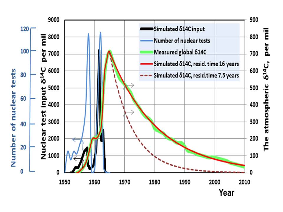
Radioactive 14C concentration decrease since 1964 shows (see figure) that the residence time of a small CO2 increase, which is not present in the atmosphere, is 16 years. No models needed, just measurements. Shorter residence times for anthropogenic CO2 are not possible, because it behaves in the same way as 14C.
The residence time of the total CO2 in the atmosphere is 55 years, because this stuff is already in the oceans and in the biosphere from where it recycles back into the atmosphere all the time. The only outlet is the flux into the deep ocean.
Aveollila,
There is a problem with 14C as representing the behaviour of the sink speed of any extra total CO2 (or 99% 12CO2):
What is going into the deep oceans near the poles is the current isotopic composition (minus the air-water isotopic shift), what comes out near the equator is the isotopic composition of ~1000 years ago (minus the water-air isotopic shift). That makes that at the height of the atomic bomb tests the 14C removed was over twice the 14C which returned (plus the 14C decay itself). The overall decay rate for 14C therefore is about 3 times the overall decay rate for any 12CO2 excess above equilibrium.
The observed excess CO2 decay rate since Mauna Loa is ~51 years, quite linear over the years…
Here the sink and source estimates for total CO2 and 14CO2 around 1960 at the maximum 14C level in the atmosphere:
http://www.ferdinand-engelbeen.be/klimaat/klim_img/14co2_distri_1960.jpg
Of 100% 12CO2 going into the deep oceans, about 97.5% is returning in the same year.
Of 100% 14CO2 going into the deep oceans, about 45% is returning in the same year.
That makes that the decay rate of any excess 14CO2 is much faster than for any excess 12CO2…
The same problem occurs with the “thinning” of the human δ13C “signal” from burning fossil fuels: the drop in δ13C is only 1/3 of what can be expected if all human induced CO2 remained in the atmosphere. As there are huge exchanges (~40 GtC/year) between the deep oceans and the atmosphere, the higher δ13C from the deep oceans removes about 2/3 of the δ13C drop…
Aveollila,
Sorry, overlooked your last paragraph, which shows that you did know the difference between 14CO2 and 12CO2 decay rates…
The problem with Tim’s as good as with the IPCC’s “residence time” is that they mix the two definitions:
– The (real) residence time = mass / throughput, which governs the fate of any individual CO2 molecule in the atmosphere, whatever its origin. That doesn’t remove or add any CO2 mass from/to the atmosphere.
– The (e-fold) decay rate is how much is removed out of the atmosphere as function of the extra CO2 pressure, whatever its origin, which is extra pressure / mass removal (or cause/effect)…
3) http://cdiac.esd.ornl.gov/ftp/ndp030/global.1751_2004.ems
From tables accessible at 2) and 3) we can do some decadal average annual analysis as:
Decade 1 2 3 4 5
Years ’54-63 ’64-’73 ’74-’83 ’84-’93 ’94-`03
Ave. annual fuel emissions (Gt/yr) 2.4 3.4 5.0 6.0 6.7
Percent change decade to decade 42 47 20 12
Ave. annual atmos. conc’n delta (ppm/yr) 0.8 1.1 1.4 1.5 1.8
Atmos. conc’n delta per Gt emission (ppB) 333 324 280 250 270
Implied atmospheric retention (Gt) 1.7 2.3 2.9 3.1 3.7
Airborne fraction (%) 71 68 58 52 55
Ocean uptake from fuel (Gt) 0.7 1.1 2.1 2.9 3.0
Deforestation factor (%) guesstimate* 1.03 1.06 1.09 1.12 1.15
Total emissions (Gt) 2.5 3.6 5.5 6.7 7.7
Airborne fraction of total (%) 68 64 53 46 48
Ocean uptake total (Gt) 0.8 1.3 2.6 3.6 4.0
*The above fuel emissions from 3) do not include any factor for deforestation/land use. Recent total emissions have been estimated by AGW advocates as slightly less than 8 Gt/yr total, giving about an additional 15% for deforestation/land use. As deforestation is to a degree linked to third world population, we can assume that factor was sequentially lower going back to prior decades. Using a higher factor for prior decades won’t change anything much. Column 3 fuel emissions data corresponds almost exactly with IPCC SAR figures.
While total average annual emissions have gone up by a factor of 3, ocean uptake has gone up by a factor of 5. That is hardly consistent with slow mixing or near saturation of surface waters. What seems to be happening is that increasing atmospheric partial pressure is increasing the rate of ocean uptake with the rate of increase slowed by surface warming/acidification.
4) http://cdiac.esd.ornl.gov/pns/faq.html
snip Q. How long does it take for the oceans and terrestrial biosphere to take up carbon
after it is burned?
A. For a single molecule of CO2 released from the burning of a pound of carbon, say from burning coal, the time required is 3-4 years. This estimate is based on the carbon mass in the atmosphere and up take rates for the oceans and terrestrial biosphere. Model estimates
for the atmospheric lifetime of a large pulse of CO2 has been estimated to be 50-200 years (i.e., the time required for a large injection to be completely dampened from the atmosphere). Snip
This range seems to be an actual range depending on time frame, rather than the uncertainty among models. [See (5) below].
5) http://www.accesstoenergy.com/view/atearchive/s76a2398.htm
For the above decades 1 through 5, we have now had 4, 3, 2, 1, and 0 half lives respectively. From 3) and 5) and using an average half life of 11 years, (based on real 14C measurement) we get a total remaining injection in 2004 from the prior 5 decades of 139 Gt, which equates to an increase in atmospheric concentration of 66 ppm. The actual increase from 1954 to 2004 was very near 63 ppm. This result lends some credibility to the 50 year atmospheric residence time estimate. [See (9) below]. A 200 year residence time gives an 81 ppm delta since 1954, which is much too high.
Surprisingly, if we go all the way back to 1750 and compute the residence time using fuel emissions only we get a value very close to 200 years. (A 40 year ½ life gives a ppm delta of 99 vs an actual of 96 using 280 ppm as the correct value in 1750). If we assume that terrestrial uptake closely matches land use emissions, (this is essentially the IPCC assumption), and we know that the airborne fraction from 1964 through 2003 had a weighted average of 58%, to
shift to a long term 40 year ½ life from a near term 11 year ½ life, we would have to have prior 40 year period weighted average airborne fractions like 80% for ’24-’63, and 90%-100% before that. Since emissions in the last 40 years have been 3 times higher than in the period from 1924 to 1963 and 30 times higher than 1844 to 1883 it is not too hard to believe that the rapid growth in atmospheric partial pressure has forced such a change in airborne fraction. With rising SSTs we can expect the partial pressure forced rate of ocean uptake to be offset to a growing degree. (Of course we now know that since 2003 we have not had rising SSTs, rather a slight cooling.)As emission rates decline in the future, and with the delayed impact of ocean warming the half life can be expected to begin growing again but it seems very unlikely that the residence time for a pulse of CO2 would get back to 200 years.
We may say that Arrhenius invented the GH phenomenon and the warming effect of CO2 but it has no impact in the present-day science of IPCC. The warming effects of CO2 can be calculated according to a very simple formula
dT = CSP * 5.35 * (CO2/280)
If the real science cannot find anything wrong with this formula, they have to say that they have no better way or they do not know what is wrong. It is not a scientific statement that CO2 has no warming effect. If you say so 1) you say that there is no GH effect, which is nonsense, 2) CO2 has a role in the GH effect but it stopped at CO2 level 280 ppm. Any other options? Yes, you can say that the increasing CO2 concentration has a warming effect but the climate system has a negative feedback feature, which eliminates all the deviations from the pre-set temperature value of 15 degrees.
My conclusion is that there is something wrong in the formula above.
“Because CO2 is such a small percentage of the greenhouse gases they created a measure called “climate sensitivity,” which claims that CO2 is more “effective” as a greenhouse gas than water vapor.”
Told to us by the same people who tell us that “All animals are equal, but some are more equal than others.”
This the first time I read that CO2 is stronger GH gas than water vapor. IPCC has many errors in its science but not this one.
Go read about the Globall Warming Potential (GWP) index. It was first used when we pointed out that Methane was a fraction of the total greenhouse gases so they said it was more effective than CO2 and it was more effective than water vapour. As I recall it is inthe IPCC Glossary.
Thanks Dr. Ball. An excellent piece.
About the CO2 GH effects. Yes, If you mean that GWEP values, then CO2 is stronger than H2O. This key figure is totally unrealistic and it is created to support AGW theory. In my mind was the contributions of GH gases in the GH effect and in this calculation H”O is stil number one.
Thank you Dr. Tim Ball. You hit the nails (all of ’em) on the head.
Regards,
WL
Reply to F Englebeen 3:41 PM I wrote the following in 2008
I went from
> Jaworowski to Beck, to RC on Beck, to Law Dome, and to
> several other sources. Seems to me that most all are right, and most all
> are wrong. To wit:
> Both Jaworowski and Beck seem to think that the measurements Beck presents
> are global, and therefore ice cores are wrong. They also are thinking
> statically rather than dynamically. RC agrees and points out, correctly,
> that there was no CO2 source that could create the 1942 peak (globally).
> Beck says the peak is not WWII because there are elevated readings in
> Alaska and Poona India.
> Let’s assume that the warm spell peaking about 1938 made a small
> contribution and WWII made a large contribution. There is no reason that
> there couldn’t have been local spikes also in Alaska (military staging)
> and Poona (industrialized part of India supporting the Asian campaign).
> Most of the measurements were from Europe, and in ’41/’42 Europe was in
> flames. Imagine a high ridge of elevated CO2 across Europe that is
> continuously flowing out to become well mixed around the world. By the
> time it gets to the South Pole 200 ppm would probably be no more than 20
> ppm.
> Now consider that a few year spike (bottom to bottom 1935 to 1952) gets
> averaged out over abouit 80 years during ice closure, so its maybe 4 ppm.
> By the time the core is made, 1942 ice is deep enough to form CO2
> clathrates, but not oxygen or nitrogen per Jaworowski, so when the core
> depressurizes, some more of the peak is lost, now 1 ppm.
> Now see Law Dome, per Etheridge “flat to slightly up and down” from about
> 1935 to 1952.
> You can take the Law Dome CO2 plot, look only at the last 100 years, and
> fit Beck’s peak right on the unexplained flat.
> There was plenty of CO2 to generate that ridge over Europe, and it was
> WWII. Beck is right, the ice core is right, RC is right; Beck is wrong, RC
> is wrong, but the ice core remains right.
> It would be nice if people didn’t jump to conclusions and would think
> dynamically.
See http://www.scribd.com/doc/147447107/Breaking-Ice-Hockey-Sticks-Can-Ice-Be-Trusted to add fractionation to the story.
Murray,
Beck’s peak is based on contaminated data, period. Poona, India, measured CO2 under, inbetween and over growing crops, nothing comparable to “background” CO2 levels.
The data from Barrow, Alaska are part of the “ugly” data, as the equipment was intended to measure the health of the researcher by measuring CO2 in their exhaled air at 20,000 to 40,000 ppmv with an accuracy of +/- 150 ppmv. That equiment was calibrated with outside air. If the reading was between 250-500 ppmv, the equipment was ready to use… It is these calibration data that Beck used as “real” outside air data…
With a minimum of qaulity control, such data would be discarded…
Even if WWII had a huge contribution, it is simply impossible that there was such a peak in CO2: 80 ppmv is the equivalent of burning 1/3 of all vegetation on earth (including tropical forests) and regrowing it all in a few years. If that was the case, that would be significant in the stomata data and the d13C drop and return. Both show zero influence around 1942.
Further, the open pores in firn allow a lot of exchange between CO2 in the pores and the atmosphere: 40 years of migration for Law Dome before closing the bubbles: The average age of the CO2 level at the bottom of the firn is only 7 years younger than in the atmosphere, not 20 years as you expect. The resolution of the CO2 in the gas bubbles is only 8 years, as that is the time period to seal all different bubbles at different time intervals. Thus if there was such a 80 ppmv, it would have given an at least 40 ppmv peak in the Law Dome ice cores… There were no clathrates neither melt layers in the Law Dome ice cores. Clathrates BTW decompose under vacuum, thus normally not a problem with the grating technique and certainly not with the sublimation technique.
About Jonthan Drake’s article: I had some discussions with him in the past where he had similar fantasies: mathematically right, but with a complete lack of cause and effect insight…
Indeed the smallest atoms and molecules show some fractionation at bubble closing time, but CO2 is not one of them. If it had an influence, CO2 levels in ice cores with enormous differences in bubble closing time should show huge differences in CO2 levels for the same average gas age and CO2 levels would decrease over time during conservation, as is the case for the O2/N2 ratio…
This is beyond a joke. Look at the data.
http://woodfortrees.org/graph/hadsst2nh/from:1880/to:1940/plot/hadsst2sh/from:1880/to:1940/plot/hadsst3nh/from:1880/to:1940
The SH data follows the NH too closely to have really been a measurement rather than calculated from NH anomalies. HadSST2 and HadSST3 NH differ much more than HadSST2SH and HadSST3NH.
There are large differences between all 4 in the period 1940-1970
http://woodfortrees.org/graph/hadsst2nh/from:1880/mean:12/plot/hadsst2sh/from:1880/mean:12/plot/hadsst3nh/from:1880/mean:12/plot/hadsst3sh/from:1880/mean:12
As a lot of people have pointed out, the integral of the GTA correlates well with CO2 levels (or the derivative of global CO2 levels correlates well with GTA). The best correlation is with HadSSTv3SH (southern hemisphere). The next best is with HadSSTv2NH, much better than HadSSTv3NH or v2SH.
http://woodfortrees.org/graph/esrl-co2/mean:12/plot/hadsst3sh/from:1959/offset:0.4/integral/scale:0.25/offset:315/plot/hadsst3nh/from:1959/offset:0.4/integral/scale:0.25/offset:330/plot/hadsst2nh/from:1959/offset:0.4/integral/scale:0.25/offset:330/plot/hadsst2sh/from:1959/offset:0.4/integral/scale:0.25/offset:330
(v2NH, v2SH and v3NH offset to show how the hemispheres are closer than the different versions)
My guess is that there needed to be a quick fix after this
https://wattsupwiththat.com/2013/11/14/curry-on-the-cowtan-way-pausebuster-is-there-anything-useful-in-it/
Only a guess but I’m pretty confident that the Keeling curve is the integral of the calculated SH SST (now) with local measurements merely noise and that the adjustments to the NH data would have made a large and noticeable change to the ESRL Mauna Loa CO2 levels if nothing were done. Someone cocked up when adjusting the NH data to kill two birds with one stone ie get rid of that 40s blip as well as the pause and a quick fix was needed.
http://woodfortrees.org/graph/hadsst2nh/from:1959/offset:0.4/integral/scale:0.25/offset:320/plot/esrl-co2/mean:12/plot/hadsst3sh/from:1959/offset:0.4/integral/scale:0.25/offset:315
I know that its harsh criticism (I will not use the F word) but this needs to come out.
Quotations from Edmund Burke (12 January 1729 – 9 July 1797)
Bad laws are the worst sort of tyranny.
Speech at Bristol Previous to the Election (6 September 1780)
Whenever a separation is made between liberty and justice, neither, in my opinion, is safe.
Letter to M. de Menonville (October 1789)
************************************************************
Data manipulation is well known and well documented. If this kind of nonsense was done in any other field there would be criminal prosecutions.
Climate Science Behaving Badly; 50 Shades of Green & The Torture Timeline
https://co2islife.wordpress.com/
Dr. Ball is certainly entitled to his opinion, and I don’t know Dr. Bates from Adam, but I think there is more to consider here. First of all, Dr. Bates likely went into his career with an affection for the environment like a lot of people wanting to “make a difference”. And let’s be honest, the question of CO2 warming the planet was at least on its face a legitimate question needing some attention within the 40 years of Dr. Bates career. And it is possible that throughout his career he has fallen victim to confirmation bias, or been in roles too junior or too isolated to allow him to fully see how all the sausage is made. In short, there is room to believe that Dr. Bates may be a good guy who just wasn’t in a position to know enough to see that something was truly wrong until relatively late in his career.
It also clear that Dr. Bates has been trying for some time to work within the system to try to reform it, raising concerns through the proper channels and championing practices that support integrity. We should also consider that until very recently with the change in administration there has been an executive branch that seen fit to ignore the will of the people, the laws on the books, and indeed the constitution whenever it suited their political agenda, and any protest Dr. Bates might have raised would have amounted to him being discredited and marginalized. What would have been the point? At least by working from within he could try to reform the process and try to limit NOAA’s ability to manipulate data.
You have to also understand working for the federal government like I do. I’ve spent most of my career in the private sector and only recently have spent a couple of years doing a federal contracting job. It was a huge culture shock. The number one question that never gets answered is “why”. Why is that process that way? Why don’t we consider any alternatives? Most people don’t know or care why. Some decision was made years ago by some bureaucrat about how and why something is done, and it is seldom questioned thereafter. It is a world where most people are just passing time waiting for their pension as their reward for enduring mindless tedium, and those who come into it with any passion or drive are quickly subdued or cast out, leaving only the bitter clingers to remain to sustain the system. Gains are measured in inches not miles, and change only seems to occur as a reaction to an absolute disaster. It is easy to understand that someone like Dr. Bates who spent his entire career in that environment was not equipped to appreciate just how out of touch NOAA is with the real world way that things are done.
So while I understand Dr. Ball’s reservation not to hoist Dr. Bates to the level of hero, I also would err on the side of not casting him as a villain. Consider that he has at least raised doubts about NOAA, which then can beg the question, “if this one example is a problem, then are there more examples? Is this a symptom of a much larger problem?” Consider also that he paved the way for others to step forward, not only at NOAA, but perhaps NASA, the EPA, etc. Even if Dr. Bates isn’t the best example of a whistle blower, he is at least the first from NOAA, and that is worthy of some acknowledgement.
If your understanding of the global carbon cycle is so base as to broadly suggest that 50% of carbon is sequestered through photosynthesis. I can’t help but wonder what else you’ve exaggerated, or misrepresented out of lack of background.
FYI 110 out of the 112.5 billion tons of C per year are sequestered by the biosphere. And this figure doesn’t actually help your theory in the slightest.
If the worlds fauna could conceivably sequester upwards of 1000 ppm co2 than there would not be a +4.5-6.5 billion tons of carbon per year in surplus after photosynthesis and carbon sinks! The plants are not starving….
About the residence time. I can just confirm the comment of Engelbeen. I have carried out my own calculations applying quite simple atmosphere-ocean-biosphere model. There are two residence times. The anthropogenic CO2 16 years, and the total CO2 55 years.