Part II: How the central estimate of pre-feedback warming was exaggerated
By Christopher Monckton of Brenchley
In this series I am exploring the cumulative errors, large and small, through which the climatological establishment has succeeded in greatly exaggerating climate sensitivity. Since the series concerns itself chiefly with equilibrium sensitivity, time-dependencies, including those arising from non-linear feedbacks, are irrelevant.
In Part I, I described a small error by which the climate establishment determines the official central estimate of equilibrium climate sensitivity as the inter-model mean equilibrium sensitivity rather than determining that central estimate directly from the inter-model mean value of the temperature feedback factor f. For it is the interval of values for f that dictates the interval of final or equilibrium climate sensitivity and accounts for its hitherto poorly-constrained breadth [1.5, 4.5] K. Any credible probability-density function for final sensitivity must, therefore, center on the inter-model mean value of f, and not on the inter-model mean value of ΔT, skewed as it is by the rectangular-hyperbolic (and hence non-linear) form of the official system gain equation G = (1 – f)–1.
I showed that the effect of that first error was to overstate the key central estimates of final sensitivity by between 12.5% and 34%.
Part II, which will necessarily be lengthy and full of equations, will examine another apparently small but actually significant error that leads to an exaggeration of reference or pre-feedback climate sensitivity ΔT0 and hence of final sensitivity ΔT.
For convenience, the official equation (1) of climate sensitivity as it now stands is here repeated. There is much wrong with this equation, but, like it or not, it is what the climate establishment uses. In Part I, it was calibrated closely and successfully against the outputs of both the CMIP3 and CMIP5 model ensembles.
(1) ![]()
where ![]()
Fig. 1 illuminates the interrelation between the various terms in (1). In the current understanding, the reference or pre-feedback sensitivity ΔT0 is simply the product of the official value of radiative forcing ΔF0 = 3.708 W m–2 and the official value of the reference sensitivity parameter λ0 = 3.2–1 K W–1 m2, so that ΔT0 = 1.159 K (see e.g. AR4, p. 631 fn.).
However, as George White, an electronics engineer, has pointed out (pers. comm., 2016), in using a fixed value for the crucial reference sensitivity parameter λ0 the climate establishment are erroneously treating the fourth-power Stefan-Boltzmann equation as though it were linear, when of course it is exponential.
This mistreatment in itself leads to a small exaggeration, as I shall now show, but it is indicative of a deeper and more influential error. For George White’s query has led me to re-examine how, in official climatology, λ0 came to have the value at or near 0.312 K W–1 m2 that all current models use.

Fig. 1 Illumination of the official climate-sensitivity equation (1)
The fundamental equation (2) of radiative transfer relates flux density Fn in Watts per square meter to the corresponding temperature Tn in Kelvin at some surface n of a planetary body (and usually at the emission surface n = 0):
(2) ![]() | Stefan-Boltzmann equation
| Stefan-Boltzmann equation
where the Stefan-Boltzmann constant σ is equal to 5.6704 x 10⁻⁸ W m–2 K–4, and the emissivity εn of the relevant surface n is, by Kirchhoff’s radiation law, equal to its absorptivity. At the Earth’s reference or emission surface n = 0, a mean 5.3 km above ground level, emissivity ε0, particularly with respect to the near-infrared long-wave radiation with which we are concerned, is vanishingly different from unity.
The Earth’s mean emission flux density F0 is given by (3),
(3)  238.175 W m–2,
where S0 = 1361 W m–2 is total solar irradiance (SORCE/TIM, 2016); α = 0.3 is the Earth’s mean albedo, and 4 is the ratio of the surface area of the rotating near-spherical Earth to that of the disk that the planet presents to incoming solar radiation. Rearranging (2) as (4) and setting n = 0 gives the Earth’s mean emission temperature T0:
(4)  254.578 K.
A similar calculation may be performed at the Earth’s hard-deck surface S. We know that global mean surface temperature TS is 288 K, and measured emissivity εS ≈ 0.96. Accordingly, (3) gives FS as 374.503 W m–2. This value is often given as 390 W m–2, for εS is frequently taken as unity, since little error arises from that assumption.
The first derivative λ0 of the Stefan-Boltzmann equation relating the emission temperature T0 to emission flux density F0 before any radiative perturbation is given by (5):
(5) 
![]() 0.267 K W–1 m2.
0.267 K W–1 m2.
The surface equivalent λS = TS / (4FS) = 0.192 K W–1 m2 (or 0.185 if εS is taken as unity).
The official radiative forcing in response to a doubling of atmospheric CO2 concentration is given by the approximately logarithmic relation (6) (Myhre et al., 1998; AR3, ch. 6.1). We shall see later in this series that this value is an exaggeration, but let us use it for now.
(6) ![]() 3.708 W m–2.
3.708 W m–2.
Then the direct or reference warming in response to a CO2 doubling is given by
(7) ![]() 0.991 K.
0.991 K.
A similar result may be obtained thus: where Fμ = F0 + ΔF0 = 238.175 + 3.708 = 241.883 W m–2, using (2) gives Tμ:
(8)  255.563 K.
Then –
(9) ![]() 0.985 K,
0.985 K,
a little less than the result in (7), the small difference being caused by the fact that λ0 cannot have a fixed value, because, as George White rightly points out, it is the first derivative of a fourth-power relation and hence represents the slope of the curve of the Stefan-Boltzmann equation at some particular value for radiative flux and corresponding value for temperature.
Thus, the value of λ0, and hence that of climate sensitivity, must decline by little and little as the temperature increases, as the slightly non-linear curve in Fig. 2 shows.

Fig. 2 The first derivative λ0 = T0 / (4F0) of the Stefan-Boltzmann equation, which is the slope of a line tangent to the red curve above, declines by little and little as T0, F0 increase.
The value of λ0 may also be deduced from eq. (3) [here (10)] of Hansen (1984), who says [with notation altered to conform to the present work]:
“… for changes of solar irradiance,
(10) ![]() …
…
“Thus, if S0 increases by a small percentage δ, T0 increases by δ/4. For example, a 2% change in solar irradiance would change T0 by about 0.5%, or 1.2-1.3 K.”
Hansen’s 1984 paper equated the radiative forcing ΔF0 from a doubled CO2 concentration with a 2% increase ΔF0 = 4.764 W m–2 in emission flux density, which is where the value 1.2-1.3 K for ΔT0 = ΔF0λ0 seems first to have arisen. However, if today’s substantially smaller official value ΔF0 = 3.708 W m–2 (Myhre et al., 1998; AR3, ch. 6.1) is substituted, then by (10), which is Hansen’s equation, ΔT0 becomes 0.991 K, near-identical to the result in (7) here, providing further confirmation that the reference or pre-feedback temperature response to a CO2 doubling should less than 1 K.
The Charney Report of 1979 assumed that the entire sensitivity calculation should be done with surface values FS, TS, so that, for the 283 K mean surface temperature assumed therein, the corresponding surface radiative flux obtained via (2) is 363.739 W m–2, whereupon λS was found equal to a mere 0.195 K W–1 m2, near-identical to the surface value λS = 0.192 K determined from (5).
Likewise, Möller (1963), presenting the first of three energy-balance models, assumed today’s global mean surface temperature 288 K, determined from (2) the corresponding surface flux 390 W m–2, and accordingly found λS = 288 / (4 x 390) = 0.185 K W–1 m2, under the assumption that surface emissivity εS was equal to unity.
Notwithstanding all these indications that λ0 is below, and perhaps well below, 0.312 K W–1 m2 and is in any event not a constant, IPCC assumes this “uniform” value, as the following footnote from AR4, p.631, demonstrates [with notation and units adjusted to conform to the present series]:
“Under these simplifying assumptions the amplification of the global warming from a feedback parameter c (in W m–2 K–1) with no other feedbacks operating is 1 / (1 – c λ0), where λ0 is the ‘uniform temperature’ radiative cooling response (of value approximately 3.2–1 K W–1 m2; Bony et al., 2006). If n independent feedbacks operate, c is replaced by (c1 + c2 +… + cn).”
How did this influential error arise? James Hansen, in his 1984 paper, had suggested that a CO2 doubling would raise global mean surface temperature by 1.2-1.3 K rather than just 1 K in the absence of feedbacks. The following year, Michael Schlesinger described the erroneous methodology that permitted Hansen’s value for ΔT0 to be preserved even as the official value for ΔF0 fell from Hansen’s 4.8 W m–2 per CO2 doubling to today’s official (but still much overstated) 3.7 W m–2.
In 1985, Schlesinger stated that the planetary radiative-energy budget was given by (11):
(11) ![]()
where N0 is the net radiation at the top of the atmosphere, F0 is the downward flux density at the emission altitude net of albedo as determined in (3), and R0 is the long-wave upward flux density at that altitude. Energy balance requires that N0 = 0, from which (3, 4) follow.
Then Schlesinger decided to express N0 in terms of the surface temperature TS rather than the emission temperature T0 by using surface temperature TS as the numerator and yet by using emission flux F0 in the denominator of the first derivative of the fundamental equation (2) of radiative transfer.
In short, he was applying the Stefan Boltzmann equation by straddling uncomfortably across two distinct surfaces in a manner never intended either by Jozef Stefan (the only Slovene after whom an equation has been named) or his distinguished Austrian pupil Ludwig Boltzmann, who, 15 years later, before committing suicide in despair at his own failure to convince the world of the existence of atoms, had provided a firm theoretical demonstration of Stefan’s empirical result by reference to Planck’s blackbody law.
Since the Stefan-Boltzmann equation directly relates radiative flux and temperature at a single surface, the official abandonment of this restriction – which has not been explained anywhere, as far as I can discover – is, to say the least, a questionable novelty.
For we have seen that the Earth’s hard-deck emissivity εS is about 0.96, and that its emission-surface emissivity ε0, particularly with respect to long-wave radiation, is unity. Schlesinger, however, says:
“N0 can be expressed in terms of the surface temperature TS, rather than [emission temperature] T0 by introducing an effective planetary emissivity εp, in (12):
(12)  0.6
0.6![]() ,
,
so that, in (13),
(13)  0.302 K W–1 m2.
This official approach embodies a serious error arising from a misunderstanding not only of (2), which relates temperature and flux at the same surface and not at two distinct surfaces, but also of the fundamental architecture of the climate.
Any change in net flux density F0 at the mean emission altitude (approximately 5.3 km above ground level) will, via (2), cause a corresponding change in emission temperature T0 at that altitude. Then, by way of the temperature lapse rate, which is at present at a near-uniform 6.5 K km–1 just about everywhere (Fig. 3), that change in T0 becomes an identical change TS in surface temperature.

Fig. 3 Altitudinal temperature profiles for stations from 71°N to 90°S at 30 April 2011, showing little latitudinal variation in the lapse-rate of temperature with altitude. Source: Colin Davidson, pers. comm., August 2016.
But what if albedo or cloud cover or water vapor, and hence the lapse rate itself, were to change as a result of warming? Any such change would not affect the reference temperature change ΔT0: instead, it would be a temperature feedback affecting final climate sensitivity ΔT.
The official sensitivity equation thus already allows for the possibility that the lapse-rate may change. There is accordingly no excuse for tampering with the first derivative of the Stefan-Boltzmann equation (2) by using temperature at one altitude and flux at quite another and conjuring into infelicitous existence an “effective emissivity” quite unrelated to true emissivity and serving no purpose except unjustifiably to exaggerate λ0 and hence climate sensitivity.
One might just as plausibly – and just as erroneously – choose to relate emission temperature with surface flux, in which event λ0 would fall to 254.6 / [4(390.1)] = 0.163 K W–1 m2, little more than half of the models’ current and vastly-overstated value.
This value 0.163 K W–1 m2 was in fact obtained by Newell & Dopplick (1979), by an approach that indeed combined elements of surface flux FS and emission temperature T0.
The same year the Charney Report, on the basis of hard-deck surface values TS and FS for temperature and corresponding radiative flux density respectively, found λS to be 0.192 K W–1 m2.
IPCC, followed by (or following) the overwhelming majority of the models, takes 3.2–1, or 0.3125, as the value of λ0. This choice thus embodies two errors one of modest effect and one of large, in the official determination of λ0. The error of modest effect is to treat λ0 as though it were constant; the error of large effect is to misapply the fundamental equation of radiative transfer by straddling two distinct surfaces in using it to determine λ0. As an expert reviewer for AR5, I asked IPCC to provide an explanation showing how λ0 is officially derived. IPCC curtly rejected my recommendation. Perhaps some of its supporters might assist us here.
In combination, the errors identified in Parts I and II of this series have led to a significant exaggeration of the reference sensitivity ΔT0, and commensurately of the final sensitivity ΔT, even before the effect of the errors on temperature feedbacks is taken into account. The official value ΔT0 = 1.159 K determined by taking the product of IPCC’s value 0.3125 K W m–1 for λ0 and its value 3.708 W m–2 for ΔF0 is about 17.5% above the ΔT0 = 0.985 K determined in (9).
Part I of this series established that the CMIP5 models had given the central estimate of final climate sensitivity ΔT as 3.2 K when determination of the central estimate of final sensitivity from the inter-model mean central estimate of the feedback factor f would mandate only 2.7 K. The CMIP 5 models had thus already overestimated the central estimate of equilibrium climate sensitivity ΔT by about 18.5%.
The overstatement of the CMIP5 central estimate of climate sensitivity resulting from the combined errors identified in parts I and II of this series is accordingly of order 40%.
This finding that the current official central estimate climate sensitivity is about 40% too large does not yet take account of the effect of the official overstatement of λ0 on the magnitude of that temperature feedback factor f. We shall consider that question in Part III.
For now, the central estimate of equilibrium climate sensitivity should be 2.3 K rather than CMIP5’s 3.2 K. Though each of the errors we are finding is smallish, their combined influence is already large, and will become larger as the compounding influence of further errors comes to be taken into account as the series unfolds.
Table 1 shows various values of λ0, compared with the reference value 0.264 K W–1 m2 obtained from (8).
| Table 1: Some values of the reference climate-sensitivity parameter λ0 | ||||
| Source | Method | Value of λ0 | x 3.7 = ΔT0 | Ratio |
| Newell & Dopplick (1979) | T0 / (4FS) | 0.163 K W–1 m2 | 0.604 K | 0.613 |
| Möller (1963) | TS / (4FS) | 0.185 K W–1 m2 | 0.686 K | 0.696 |
| Callendar (1938) | TS / (4FS) | 0.195 K W–1 m2 | 0.723 K | 0.734 |
| From (8) here | T0 / (4F0) | 0.264 K W–1 m2 | 0.985 K | 1.000 |
| Hansen (1984) | T0 / (4F0) | 0.267 K W–1 m2 | 0.990 K | 1.005 |
| From (7) here | T0 / (4F0) | 0.267 K W–1 m2 | 0.991 K | 1.006 |
| Schlesinger (1985) | TS / (4F0) | 0.302 K W–1 m2 | 1.121 K | 1.138 |
| IPCC (AR4, p. 631 fn.) | 3.2–1 | 0.312 K W–1 m2 | 1.159 K | 1.177 |
Nearly all models adopt values of λ0 that are close to or identical with IPCC’s value, which appears to have been adopted for no better reason that it is the reciprocal of 3.2, and is thus somewhat greater even than the exaggerated value obtained by Schlesinger (1985) and much copied thereafter.
In the next instalment, we shall consider the effect of the official exaggeration of λ0 on the determination of temperature feedbacks, and we shall recommend a simple method of improving the reliability of climate sensitivity calculations by doing away with λ0 altogether.
I end by asking three questions of the Watts Up With That community.
1. Is there any legitimate scientific justification for Schlesinger’s “effective emissivity” and for the consequent determination of λ0 as the ratio of surface temperature to four times emission flux density?
2. One or two commenters have suggested that the Stefan-Boltzmann calculation should be performed entirely at the hard-deck surface when determining climate sensitivity and not at the emission surface a mean 5.3 km above us. Professor Lindzen, who knows more about the atmosphere than anyone I have met, takes the view I have taken here: that the calculation should be performed at the emission surface and the temperature change translated straight to the hard-deck surface via the lapse-rate, so that (before any lapse-rate feedback, at any rate) ΔTS ≈ ΔT0. This implies λ0 = 0.264 K W–1 m2, the value taken as normative in Table 1.
3. Does anyone here want to maintain that errors such as these are not represented in the models because they operate in a manner entirely different from what is suggested by the official climate-sensitivity equation (1)? If so, I shall be happy to conclude the series in due course with an additional article summarizing the considerable evidence that the models have been constructed precisely to embody and to perpetuate each of the errors demonstrated here, though it will not be suggested that the creators or operators of the models have any idea that what they are doing is as erroneous as it will prove to be.
Ø Next: How temperature feedbacks came to be exaggerated in official climatology.
References
Charney J (1979) Carbon Dioxide and Climate: A Scientific Assessment: Report of an Ad-Hoc Study Group on Carbon Dioxide and Climate, Climate Research Board, Assembly of Mathematical and Physical Sciences, National Research Council, Nat. Acad. Sci., Washington DC, July, pp. 22
Hansen J, Lacis A, Rind D, Russell G, Stone P, Fung I, Ruedy R, Lerner J (1984) Climate sensitivity: analysis of feedback mechanisms. Meteorol. Monographs 29:130–163
IPCC (1990-2013) Assessment Reports AR1-5 are available from www.ipcc.ch
Möller F (1963) On the influence of changes in CO2 concentration in air on the radiative balance of the Earth’s surface and on the climate. J. Geophys. Res. 68:3877-3886
Newell RE, Dopplick TG (1979) Questions concerning the possible influence of anthropogenic CO2 on atmospheric temperature. J. Appl. Meteor. 18:822-825
Myhre G, Highwood EJ, Shine KP, Stordal F (1998) New estimates of radiative forcing due to well-mixed greenhouse gases. Geophys. Res. Lett. 25(14):2715–2718
Roe G (2009) Feedbacks, timescales, and seeing red. Ann. Rev. Earth Planet. Sci. 37:93-115
Schlesinger ME (1985) Quantitative analysis of feedbacks in climate models simulations of CO2-induced warming. In: Physically-Based Modelling and Simulation of Climate and Climatic Change – Part II (Schlesinger ME, ed.), Kluwer Acad. Pubrs. Dordrecht, Netherlands, 1988, 653-735.
SORCE/TIM latest quarterly plot of total solar irradiance, 4 June 2016 to 26 August 2016. http://lasp.colorado.edu/data/sorce/total_solar_irradiance_plots/images/tim_level3_tsi_24hour_3month_640x480.png, accessed 3 September 2016
Vial J, Dufresne J, Bony S (2013) On the interpretation of inter-model spread in CMIP5 climate sensitivity estimates. Clim Dyn 41: 3339, doi:10.1007/s00382-013-1725-9
Thanks to Christopher Monckton and the other contributors to this thread. This back and forth, is the way things are eventually figured out. Very healthy for science.
I would like to commend Christopher Monckton for his patience in the face of provocation, and would like to request that all who diagree with him, do so without being disagreeable.
Personal attacks smack of desperation.
But it would seem that rebuttals of the good lords personal attacks, even without expletives, are not permitted on this site. Apparently there is no right of reply here. No censorship on this site. HAHA
[???? .mod]
Though I’m not always 100% happy with moderation here I would not say I see any censorship. Maybe you have something specific you wish to cite rather than such meaningless blanket accusations.
HAHA, indeed. Very funny. Now if you have something specific …
Alex,
You’re not making sense. Just because you believe something to be true, that doesn’t make it true.
You say there’s no right of reply—in your reply. Think about it.
My reply didn’t appear higher up in the thread. I was accused of being a CAGW person. When I responded, nothing happened ie appeared and disappeared. I made other comments later to other people,and they appeared. I’m not bothering with repeating what I said to the lord.
Perhaps it was one of those comments that disappear because of a glitch- in which case I apologise to the mods.
I don’t wish to discuss the matter any further.
I checked the spam que and banned words moderation filter que, and it is not in either of those. I suspect it never got submitted. It happens sometimes. It may also have something to do with the fact that your IP address says you are in China. It may be that the “great firewall of China” didn’t allow your post to be submitted in the first place.
Is this what you submitted at 6:21 AM here? If so, it seems to have gone through. Maybe you just didn’t refresh/scroll.
Since all your other posts got through it is likely that you used a banned word. This may be quite innocently. Don’t make sweeping conclusions from one post going missing.
“I don’t wish to discuss the matter any further.”
Very wise. At least we see you are not being censored as you had imagined to be the case.
“Thanks to Christopher Monckton and the other contributors to this thread. This back and forth, is the way things are eventually figured out. Very healthy for science.”
This stuff was worked out years ago, Christopher Monckton just hasn’t understood how the calculations were done, see e.g. Soden & Held (2006).
Scientists are now working on far more advanced details to improve these calculations further. They tend to do this in the peer-reviewed literature and conference proceedings rather than blogs though.
This stuff may have been worked out years ago, but some of it was worked out wrongly years ago and has remained wrong ever since.
… but some of it was worked out wrongly years ago and has remained wrong ever since
But where did Mr Monckton of Brenchley manage until now to give us any scientifically unfalsifiable proof of that?
“This stuff may have been worked out years ago, but some of it was worked out wrongly years ago and has remained wrong ever since.”
You’ve pointed out what you think is wrong with an introductory level model that scientists already know is oversimplified and gives a different result from full calculations.
Do you agree that the Soden & Held method directly answers the question: “what is the global-mean change in net flux at the top of the atmosphere when surface temperatures change by an average of 1 K?”
MieScatter continues to miss the central point I am making, which is that the determination of the reference sensitivity should be performed solely at the emission altitude, so that, with the lapse-rate held fixed, the temperature change at that altitude is the temperature change at the surface. Then, any lapse-rate changes that might occur as a result of the reference temperature change are correctly treated as part of the lapse-rate feedback. But that is not the regime described by Soden & Held, now, is it?
Monckton of Brenchley: you’re claiming that Soden & Held change the lapse rate. They don’t, read the Methods section.
Do you accept that the lapse rate is held constant?
“But that is not the regime described by Soden & Held, now, is it?”
What S&H describe in their Methodology is nothing like what you have been saying. Here it is:
They aren’t dealing with a supposed emitting surface. They aren’t even using a global effective emitting temperature. Using the GFDL GCM grid, they vary the temperature level by level, and that gives them the rate of change per that level k. That is the radiative calculation, and as per their factorisation, it does not need to be done over a long period. Then they take the long term GCM results and subtract the century difference (2110-2100 from 2010-2000) and that gives the climate rate of change of T_k relative to T_S. That gives a complete representation of the effects of temperature at different levels on surface, and gives the information needed to separately determine λ₀ and λ_L, according to the partitioning described thus:
Two distincts methods,
same answer.
So now, lets take a look at the last figure.
(CRF is … CRE)
Mr Stokes can wriggle all he wants, but Soden and Held’s values for lambda-zero make it quite plain that they are not determining those values either from the surface flux and temperature or from the emission-surface flux and temperature 5 km further up. They are are taking flux from further up and temperature from the surface. That is not a correct implementation of the SB equation, and it leads to a considerable and erroneous exaggeration of climate sensitivity.
“Mr Stokes can wriggle all he wants, but Soden and Held’s values for lambda-zero make it quite plain that they are not determining those values either from the surface flux and temperature or from the emission-surface flux and temperature 5 km further up. They are are taking flux from further up and temperature from the surface.”
Not wriggling – I’m actually reading the paper to find out what they did. You should try it. I thought at first that they used an average change T_0 and multiplied it by a derivative of F wrt that average. Approximating the average of the product with the product of the averages. But they did the correct thing of working out the product for local cell/time combinations where temperature could be assumed uniform, and averaging those products. As you note it gives a similar result. Using the product of averages for average of products is unreliable, but often does work out the same, as here.
In reply to Mr Stokes, here is what Soden & Held actually say they are doing:
“We define feedbacks in terms of the change in global mean surface temperature T(s) and the change in radiative flux at the top of the atmosphere (R).”
That approach, which derives from Schlesinger (1985) as explained in the head posting, is an abuse of the fundamental equation of radiative transfer, in which the feedbacks should be defined in terms of the changes in temperature and in flux density at the same surface and not at different surfaces.
“here is what Soden & Held actually say they are doing”
That is not what “they are doing”. It’s the definition of feedback and sensitivity. Everyone’s definition. From the AR5 glossary:
It’s just relating two separate quantities. There is no reason why they should be measured at the same place.
Monckton of Brenchley September 4, 2016 at 3:26 pm
MieScatter continues to miss the central point I am making, which is that the determination of the reference sensitivity should be performed solely at the emission altitude, so that, with the lapse-rate held fixed, the temperature change at that altitude is the temperature change at the surface. Then, any lapse-rate changes that might occur as a result of the reference temperature change are correctly treated as part of the lapse-rate feedback.
Well the emission altitude of CO2 is about 12.5km (T=~220K) so in order to determine the sensitivity to added CO2 why don’t you determine it there?
Phil: “Well the emission altitude of CO2 is about 12.5km (T=~220K) so in order to determine the sensitivity to added CO2 why don’t you determine it there?”
The feedbacks are separated from forcings, so that bit doesn’t matter.
You’re right that the “emission altitude” changes: at different altitudes it’s dominted by different gases or, in the window channels, the surface, which is why Soden & Held did the calculation the way they did. They account for a uniform warming up through the atmosphere, holding everything else constant (including the lapse rate, despite Monckton’s confusion).
If you look at their figures you can see that they include contributions from every level of the atmosphere, which is what you would get for a change in temperature. They also account for absorption above each layer of the atmosphere, which is what happens in the real world but not in Monckton’s introductory level equation.
Their calculation involves accounting for how absorption and emission depend on frequency and the abundance of emitters. It involves solving the full radiative transfer equation accounting for Planck’s law, because the loss of information from integrating it to the Stefan-Boltzmann equation means you can’t get the right answer for a nonuniform, spectrally-dependent case like the real atmosphere. Despite what Monckton says.
A comment at Nick Stokes’ blog shows that if the layer around 500 hPa (Monckton’s “emission surface”) warms by 1 K, then top-of-atmosphere emission changes by about 0.3 W m-2. The rest of the 2.8 W m-2 comes from other altitudes, including CO2 emission higher up.
MieScatter September 6, 2016 at 7:42 pm
Phil: “Well the emission altitude of CO2 is about 12.5km (T=~220K) so in order to determine the sensitivity to added CO2 why don’t you determine it there?”
The feedbacks are separated from forcings, so that bit doesn’t matter.
You’re right that the “emission altitude” changes: at different altitudes it’s dominted by different gases or, in the window channels, the surface, which is why Soden & Held did the calculation the way they did. They account for a uniform warming up through the atmosphere, holding everything else constant (including the lapse rate, despite Monckton’s confusion).
Yes, I know, I was trying to get Monckton to see the error of his ways (fat chance)!
You know, I think you’re right, Monkton is in error. No matter which way I do the math I get less than 0.18 for sensitivity. If I do it linearity I get about 0.13, if I do it from instrument malfunction I get a 0.06 , if I look at from Mt Pinatubo it’s, 2 w/m^2 and a 0.3 C drop makes, it 0.15 sensitivity. And if I do it from the real w/m^2 incoming 238 and out going at 235 that’s a big difference at calculating it 242 w/m^2, a drop of about 5 w/m^2. Which is an over estimation of about 0.7 C from Pinatubo, and a 0.65 from doing it from linear, drop from instrumention of about 0.3 C , and if we use the IPCC number of 0.6 about 3.0 C . I don’t know, you choose which story you want to tell. You tell me looking at what the modeled increase in temperature should have been, and the real world increase in temperature?
Let me be clear on this, I’m just playing along with your numbers. I actually think that co2 climate sensitivity is so low that’s it’s background noise.
Many thanks to TA for his kind words.
” 2. One or two commenters have suggested that the Stefan-Boltzmann calculation should be performed entirely at the hard-deck surface when determining climate sensitivity and not at the emission surface a mean 5.3 km above us. Professor Lindzen, who knows more about the atmosphere than anyone I have met, takes the view I have taken here: that the calculation should be performed at the emission surface and the temperature change translated straight to the hard-deck surface via the lapse-rate, so that (before any lapse-rate feedback, at any rate) ΔTS ≈ ΔT0. This implies λ0 = 0.264 K W–1 m2, the value taken as normative in Table 1.”

I was one of those.
Why? Because the Lapse Rate feedback is WRONG in the theory.
IPCC AR5 has bumped up the lapse rate feedback from -0.6 W/m2 (in AR4) to -0.9 W/m2 (in AR5). This signals that the “lapse rate’ will decrease from 6.5 C/km to about 6.3 C/km in the short medium term.
LR in this table.
http://jo.nova.s3.amazonaws.com/graph/atmosphere/hot-spot/ipcc-ch-9-feedbacks-a.gif
This means that they are predicting the “surface” will warm less fast than the troposphere shown in this graphic. The negative lapse rate feedback here.
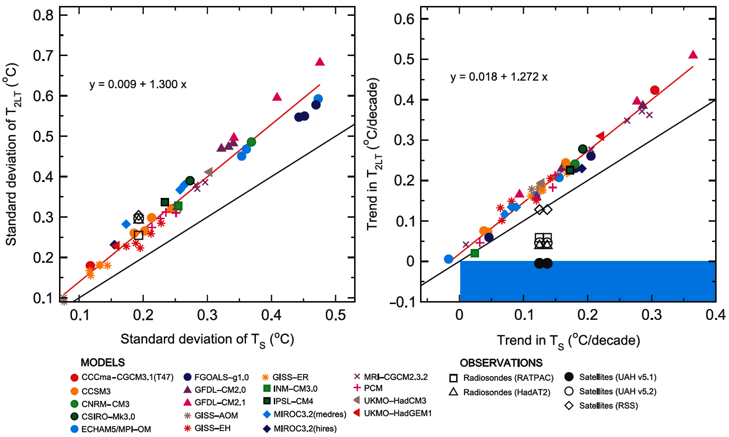
The actual value is that the troposphere will warm by 1.3 times more than the surface. This is from Thorne 2011. The trend at the 2LT (the level of UAH and RSS satellites) should warm by 1.3 times that the surface in the climate models. We used to describe this as the “tropospheric hotspot”
But the “opposite” is actually happening.
The troposphere is warming less fast than the surface. The Lapse Rate feedback is not “negative”, it is positive. The Lapse rate has actually changed from 6.5 C/km to 6.6 C/km since 1979.
In other words, throw out the lapse rate feedback and move everything back to the surface where we live.
Sorry, I meant to say “IPCC AR5 has reduced the lapse rate feedback to -0.6 W/m2 (in AR5) from -0.9 W/m2 (in AR4).
Bill Illis makes an interesting point. Similar points could be made about the other individual feedbacks, in which there is both an inter-model spread and an inter-ensemble spread.
There is growing evidence, for instance, that the water vapor feedback is not occurring at all (see NOAA’s water vapor project graphs for the past 30 years, or those of ISCCP). Therefore the lapse-rate feedback, which originally depended in no small measure on the models’ now proven-incorrect assumption that the tropical mid-troposphere would warm at twice or even thrice the tropical surface rate, is going to have to be scaled back.
Frankly, all of the official climate-sensitivity calculations are a mess. And just watch out for the revelations yet to come.
While the surface temperature measurements (GISS, NOAA, HadCRUT4, BEST) grossly agree, with the exception of JMA being a bit cooler, we actually experience stronger differences between UAH6.0 and RSS4.0 (for which the TLT variant still is not in op).
We can’t compare them using Paul Clarke’s WFT, but when using RSS3.3 TTT which is here nearly identical to UAH6.0beta5, we can do it very well at Kevin Cowtan’s trend computer, from 1979 till present:
– RSS3.3 TTT: 0.123 ± 0.060 °C/decade (with TLS insemination)
– RSS4.0 TTT: 0.176 ± 0.061 °C/decade (TLS insemination reduced)
By comparing that with
– GISS l+o: 0.171 ± 0.040 °C/decade
we see that both surface and troposphere would seem to warm quite similar in case of RSS4.0 being over the long term the more correct appreciation for tropospheric temps. Wait and see.
wait and see ? for how long should we wait and see.
for how long should we wait and see.
At least as long as
– Remote Sensing Sytems needs to publish RSS4.0 TLT;
– experts manage to compare peer-revied papers from UAH and RSS.
The latter point has recently become more and more possible.
Please compare
http://www.drroyspencer.com/2016/08/uah-global-temperature-update-for-july-2016-0-39-deg-c/
hinting on
Note we are now at “beta5” for Version 6, and the paper describing the methodology is
still in peer review.
with
http://www.drroyspencer.com/2016/09/uah-global-temperature-update-for-august-2016-0-44-deg-c/
hinting on
Note we are now at “beta5” for Version 6, and the paper describing the methodology is
back to the journal editors from peer review.
That needed well oh well a lot of time.
The analysis does not change when observations do not support the theory in question. Paradoxes and anomalies occur when a theory is incorrect.
The troposphere is warming less fast than the surface and (I repeat, AND) the majority of the warming that has occurred is occurring at high latitude regions. Global warming is not global. It is latitude specific. As atmospheric CO2 is evenly distributed in the atmosphere the change in forcing for an increase in atmospheric CO2 should cause global warming, not latitude specific warming.
P.S.
The upper troposphere has cooled which is caused by less reflected sunlight off of clouds. The incoming sunlight and reflected sunlight warms the upper troposphere due to absorption of ozone.
Latitudinal specific warming (as opposed to global warming) and the fact that the troposphere is warming less fast than the surface along with satellite data (cloud cover has decreased in high latitude regions) in peer reviewed papers supports the assertion that the warming in the last 150 years was caused by changes in cloud cover, not due to the increase in atmospheric CO2.
There are cycles of high latitude warming and cooling in the paleo record (both hemispheres) which correlates to solar cycle changes.
The lapse rate in the troposphere is definitely increasing, as you say. Whether we should count only the surface not so sure.

Here is modtran looking up and down from the reputed mean ERL of 5.3 km:
It is very interesting that at this altitude up and down CO2 band intensity matches the altitude exactly, but no other ghg’s do. Despite the intensity/altitude match, the CO2 up and down fluxes are still wildly out of balance. Such balance takes place about 8km.
Yet unless one is arguing for emergent effects, we are talking about adding more CO2, pure and simple. The ERL of the CO2 bands is not 5.3km and it is not 8km. It is above 13km in that little vertical zone where the temperature ceases to “lapse” with altitude altogether, and above which it increases.
Bill Illis: Why? Because the Lapse Rate feedback is WRONG in the theory.
Thank you for your comment.
“The troposphere is warming less fast than the surface. The Lapse Rate feedback is not “negative”, it is positive. The Lapse rate has actually changed from 6.5 C/km to 6.6 C/km since 1979.”
How did you match up modelled layers to the MSU kernels? What are the uncertainties in your values?
Less divergence with SST’s only, but it’s still just there:
http://www.woodfortrees.org/graph/uah6/from:1979/plot/hadsst3gl/from:1979/plot/uah6/trend/plot/hadsst3gl/from:1979/trend
OK. I try to read everything you write here at WUWT Lord Moncton. I just finished this article.
1) are the computer models used by the UN still using James Hansen’s 1984 value? 1.2-1.3 K ΔT0=1.2-1.3 K ? I assume they are using the linear model as well.
2) The sensitivity equations that you propose is insufficient to align historical predictions of now to now data correct? So the sensitivity gap is a contributor to the overall error between the prediction and observed T?
finally 3) “committing suicide in despair at his own failure to convince the world of the existence of atoms”
I hope you don’t suffer such a thin skin! 🙂
In answer to Mr Westhaver, whom I congratulate on struggling through the rather detailed head posting:
1) The models are indeed using (or, at least, in their manner of operation reflecting) a reference sensitivity parameter lambda-zero that is equal to 0.3125 K/W/m2, which, when multiplied by the CO2 radiative forcing 3.708 W/m2, gives a reference or pre-feedback warming of 1.2 K, in line with Hansen’s 1.2-1.3 K. In truth, this value should be just under 1 K.
In answer to Mr Westhaver’s further questions:
2) Since my results will show climate sensitivity to be considerably below the current official estimates, there is of course a far better correspondence between prediction and reality in my model than in that of IPCC.
3) I have no plans at present to commit suicide, since I am far too interested in watching world events unfold.
Thank-you Lord Monckton of Brenchley. I pray that James Hansen suffers a dream like Nebuchadnezzar, that his gold head will be subject to his feet of iron and clay.
“1) are the computer models used by the UN still using James Hansen’s 1984 value? 1.2-1.3 K ΔT0=1.2-1.3 K ? I assume they are using the linear model as well.”
No. The Methods section here explains the Soden & Held (2006) calculations:
http://citeseerx.ist.psu.edu/viewdoc/download?doi=10.1.1.444.1470&rep=rep1&type=pdf
The calculation is nothing like the simplified equations shown in this blog post. For example, this equation is solved at every level in the troposphere at each location on Earth:
https://en.wikipedia.org/wiki/Radiative_transfer#The_equation_of_radiative_transfer
MieScatter uses a device common among unquestioning defenders of the Party Line: that the models are complex and therefore more likely to be right than the analysis here, which is simple. If, as he now says, radiative-transfer calculations are done at each altitude in the troposphere, then the mid-troposphere value for the first differential of that equation would be approximately the right value. Certainly all values for altitudes below the emission altitude of around 5 km would be lower than the value for that altitude.
Like it or not, the models assume a value for lambda-zero that is contrived from surface temperature and emission-altitude flux. That is what Soden and Held say is going on. That is what Schlesinger (1985) says is going on. That methodology is erroneous and leads to a considerable overstatement of climate sensitivity.
Regarding the surface equivalent of Equation 5 yielding a pre-feedback climate sensitivity of .192 K W^-1m^2 or .192 K / (W/m^2): That is .192 degree per 1 W/m^2 change in solar radiation alone. But this causes a change in outgoing longwave radiation from the surface, some of which is absorbed by greenhouse gases aloft and radiated back towards the surface. So the climate sensitivity before effects of albedo change, change of lapse rate, change of water vapor concentration, etc. (which are what are usually counted as feedbacks) is substantially more than .192 K W^-1-m^2.
In answer to Mr Klipstein, the sensitivity calculation is properly performed at the emission altitude, where the change in radiation is represented by a change in temperature, giving around 0.264 K/W/m2, which is indeed substantially more than 0.192; though there is a good case for saying that the latter value rather than the former should be used in feedback calculations (though this is not a case I shall be making here).
There is some uncertainty with regards to the lapse rate. This uncertainty and its effect on heat flux is also interconnected with clouds, especially in the lower troposphere(low clouds/cumulus). Increasing surface temperatures and dew points without an equivalent increase aloft, will steepen the lapse rate(positive feedback). This in turn, should lower the LCL(lifting condensation level) and result in more cumulus, especially those that form from rising air as a result of solar radiation heating the surface.
This in turn creates a negative feedback from cumulus forming earlier in the day and covering more of the daytime sky, blocking the more powerful SW radiation from reaching the surface. A positive contribution from trapped LW radiation takes place, which at night is the main effect from clouds.
There are a number of complicating factors that contribute to moisture and clouds. A greening of the planet has increased evapotransiration. A massive draw on aquifer/under water brought to the surface as well as other major regional changes in vegetation from crops and deforestation, ocean evaporation and changes in soil moisture from regional precipitation/weather changes.
These all have an effect on lower level moisture, which in most cases is a positive contribution. The real world effect should be and is verifying as a decrease in the diurnal temperature spread………positive effect on temperatures at night, negative during the day. Record warmth for nighttime temperatures is far exceeding new record highs in fact.
So how much of this is a contribution from the increase in water vapor seen as a positive feedback by itself in the models and how much is this effected by the changes in clouds?
Let’s say that we could in fact represent the lapse rate accurately with the right equations in the models………..in a cloud free atmosphere. The effect of cloud changes on heat flux, by themselves could be as great as the difference between the values being used to represent the lapse rate.
But then, low clouds, will greatly effect the lapse rate. Parcels rising at the moist adiabatic rate will have a different lapse rate in clear air, that is able to entrain drier air and result in a less than moist adiabatic rate than those that are in a deep cloud with a different entrainment dynamic after condensation.
These differences cannot be modeled.
I should adjust that to: some of these differences can’t be accurately represented as they are/will be occurring in the atmosphere in models(you can model anything).
Mike McGuire: There is some uncertainty with regards to the lapse rate.
That was a good comment. Thank you.
Would you happen to know who first wrote that cloud cover would be increased early in the day, causing a subsequent reduction in SW radiation to the Earth surface?
“who first wrote that cloud cover would be increased early in the day, causing a subsequent reduction in SW radiation to the Earth surface?”
Meteorology 101………..sort of. However, there are so many complicating factors………latitude and time of year for instance. Lows clouds in the higher latitudes, where the sun angle is low would not reduce SW radiation as much as in the tropics.
During Winter, when there is very little SW radiation to block, low clouds would serve mainly as trapping outgoing LW radiation in the higher latitudes.
This is consistent with observations of more warming in the coldest months of the higher latitudes.
Low clouds in the tropics would block enough SW radiation to cool the surface more. On balance, over the entire planet, what does this leave us? For sure less of a meridional temperature gradient. Then, with less of a horizontal temperature gradient in the atmosphere there is an effect on the movement of heat from areas of excess to areas of deficit.
The assumption that I am making based on 34 years as an operational meteorologist is that, with all else being equal(vertical velocities/lift for instance) regionally, if you add moisture to the air mass, whether it be from increased evapotranspiriation from a massive, densely packed corn crop in the Midwest or from a recent, widespread rain event over a large region, the lifting condensation level will be lower………moisture will condense out at a higher temperature/lower altitude and earlier in the day.
On a planetary scale, increasing water vapor should also do this. More low level cumulus clouds at the very least.
Then, there’s the contribution to increases in precipitation micro-physics that Dr. Spencer understands better than me:
http://www.drroyspencer.com/2014/09/water-vapor-feedback-and-the-global-warming-pause/
Related to just the US Cornbelt in the growing season, this is an interesting discussion about how corn evapotranspiration has created a “micro-climate”
https://www2.ucar.edu/atmosnews/perspective/4997/corn-and-climate-sweaty-topic
Christopher Monckton of Brenchley, thank you for your essay, once again.
Christopher Monckton of Brenchley, I also appreciate your informative replies to the critical comments. I think that the interchanges are mostly illuminating. I look forward to the next in this series.
Many thanks for your kind comments.
Nick Stokes
September 4, 2016 at 3:28 am
Thanks Nick. So that makes λ0 and output of the models. So is it also an input parameter as CoB is suggesting?
Greg,
No, GCMs do not use notions of feedback at all. I supported your view of that point here
Mr Stokes is being disingenuous. The models are constructed in such a way as to embody the mechanisms of feedback, though the feedbacks themselves are not stipulated as inputs. However, precisely because the models embody feedback mechanisms (such as, for instance, the water vapor feedback), it is possible for papers such as Soden & Held (2006) and Vial et al. (2013) to discern the values of the feedbacks from the models. See also AR5, fig. 9.43a, where the feedbacks thereby deduced are illustrated by IPCC.
“though the feedbacks themselves are not stipulated as inputs”
No you are being diseneguous MoB as is you usual want
As Nick Stokes says and which you do in your usual around the houses non- answering *refutation* – the feed-back parameter in the models is an emerging property of them. It drops out at the end. Not imputed AS A NUMBER at the start.
Which is what you do, and is non-physical.
That can actually be decoded as an admission when descrambling your wordage.
Look, just say it out loud my Lord, even the plebs know that honesty is what maketh the man.
toneb says it “drops out at the end”. how apt.
Toneb contributes nothing useful to the discussion. As will become apparent when I eventually reach the argument about feedbacks – which has not yet been covered in this series – there are some grave errors in the models’ handling of feedbacks. These errors are errors regardless of whether feedback values are input into the models or deduced from their output.
At its simplest, the warming without feedbacks is about 1 K. Any model that predicts equilibrium warming of more than 1 K contains routines that – by whatever method – take account of the existence of temperature feedbacks. At present, it is the view of the climatological community that there is an appreciable risk of feedback values elevated enough to cause even as much as 10 K global warming per doubling of CO2 concentration. Once I get to the argument about feedbacks, I shall demonstrate that any such conclusion is based on a large error in the determination of feedbacks. Take away the error and the probability of very high warming in response to doubled CO2 becomes vanishingly different from zero.
Toneb, in attempting to attack my argument on the feedback question before I have made it, is indicating prejudice.
Lord Monkton
Why do you respond so agressively to ToneB when all he has done is respond to your comment about feedback?
As a reminder, you said to Nick Stokes “The models are constructed in such a way as to embody the mechanisms of feedback, though the feedbacks themselves are not stipulated as inputs. However, precisely because the models embody feedback mechanisms (such as, for instance, the water vapor feedback), it is possible for papers such as Soden & Held (2006) and Vial et al. (2013) to discern the values of the feedbacks from the models. See also AR5, fig. 9.43a, where the feedbacks thereby deduced are illustrated by IPCC.”
” there are some grave errors in the models’ handling of feedbacks”
Again, GCMs do not handle feedbacks. They solve on a grid locally equations involving conserved quantities (radiation is a bit different). Feedback is a diagnostic tool. You try to fit the GCM results to a conceptual model of the way you think it ought to work. If you find that unsatisfactory, it may indicate a model failing. But also your fitting may have gone wrong, or the conceptual model may be inappropriate. Here the model seems at least over simplified.
Mr Stokes continues to be disingenuous. Of course the official climate-sensitivity equation that I have presented is simple: and yet, when calibrated against the models’ outputs deduced in Soden & Held (2006) and in Vial et al (2013) and encapsulated in AR5 (fig. 9.43a), it reproduces the published CMIP3 and CMIP5 exactly. So simplicity is not a hindrance to the purpose of the simple official equation, which is presented in the documents of IPCC. If Mr Stokes does not like the equation, let him address his concerns to the IPCC secretariat.
Now, either the models do contain routines that in some fashion allow for the existence and approximate magnitudes, in which event the simple equation (1) in the head posting will faithfully reproduce the feedbacks officially deduced from their outputs, or they do not, in which event they will simply predict the reference warming with no effect from feedbacks.
In fact, the warming they predict is plainly substantially greater than the reference warming, from which it is not rocket science to deduce that they contain processes and routines that reflect feedbacks. There is a very considerable literature on this: indeed, AR5 mentions the word “feedback” more than 1000 times.
Once the simple equation (1) has been calibrated against the models’ oficially-published outputs and has been found to reproduce their intervals of predicted climate sensitivity more or less exactly, it is then possible to examine various errors in the magnitudes of the variables or in the methods used, in order to find out what sensitivities would have emerged from the same simple equation (1) – amended where necessary to eradicate the errors.
That is a perfectly logical exercise; and, when all the errors have been revealed and discussed, those who have sworn blind that there are no errors may find themselves compelled to think again, and the architecture of the models is – in at least one major respect – going to have to be revised quite substantially. But more of that later in the series.
So far, I have established that even quite minor errors in the official methodology lead to quite large overstatements of climate sensitivity.
Similar explorations: Common errors in the use of the Stefan-Boltzmann equation Jinan Cao 2012
It’s remarkable that Germanic philosophers like Ernst Mach doubted that atoms existed as late as 1906, at least, yet British experimental physicists had already shown that not only atoms but subatomic particles indubitably exist. J. J. Thomson, for instance, demonstrated the existence of electrons in 1897.
It’s telling that Boltzmann was heavily influenced by British science, in particular Charles Darwin, and of course John Dalton, father of modern atomic theory, who died the year Boltzmann was born.
Many thanks to those who answered my earlier question. My area of ignorance is appropriately reduced.
As for an effective surface emissivity based on outgoing IR to space and surface temperature: I don’t think that is an incorrect concept, and here’s why:
Given IR leaving the planet and its atmosphere at 238.175 W/m^2 and an effective temperature at the effective radiating altitude being 254.578 K, surface temperature 288 K, surface emissivity being .96, and the surface radiating 374.503 W/m^2: This means the 238.175 W/m^2 of IR going to space (some from the atmosphere rather than the surface) is 63.6% of what the surface radiates, or 61.1% of what the surface would radiate at 288 K if its emissivity was 1.
Suppose solar output increases enough to cause the amount absorbed by the earth and the atmosphere to increase by 1 W/m^2 from 238.175 to 239.175 W/m^2. Assume absorptions and emissivities of the earth and the atmosphere don’t change, and the spectral shift of the IR radiation is negligible. The ratio of IR radiating to space from the earth/atmosphere to IR radiating from the surface would be unchanged at .636 (63.6%).
239.175/238.175 is a .41986% increase in W/m^2, so accomplishing this and maintaining equilibrium requires a temperature increase of .1048%. With ratio of radiation intensity from the surface to radiation intensity going out to space unchanged, the surface temperature also increases by .1048%. The temperature at the effective radiating altitude would increase from 254.578 to 254.8448 K (.2668 K increase), and the surface temperature would increase from 288 to 288.3018 K (.3018 K increase).
This does not require an increase of the lapse rate, because the part of the atmosphere that is below the effective radiating altitude has thermal expansion of .1048%.
.3018 K surface temperature change from a solar radiation reception change of 1 W/m^2 is close to the .312 K/w/m^2 “official figure” for pre-feedback climate sensitivity.
Average surface emissivity is known to 2 significant figures and you are comfortable in quoting 6 significant figures for the outgoing radiation?
We all here copy and paste sometimes what Excel computes for us with four digits btdp out of numbers showing only one.
Bindidon,
“…what Excel computes for us…”
And I think that it is the Achilles Heel of those who make such claims as “The hottest year/month on record.” We often get sloppy and don’t do a post-calculation analysis of the justifiable significant figures in our answers. This results in claims that can’t be supported.
You are here exxagerating the role of a few digits after the decimal point.
And to focus on the main matter: those who make such claims as “The hottest year/month on record” would never obtain any attention if the media weren’t all the time looking for such “information”, above all endless replicated on the Internet.
“a few digits after the decimal”. Are you aware of how Lorenz discovered chaos & the “butterfly effect”?
I just noticed that I came up with a figure pretty much matching Schlesinger’s. This means there is a scientific basis for it.
My good Count,
Here I was, trying to get to sleep, but I cannot rest.
Physics.
An earlier commenter asked about “Saturation.” You may or may not understand that the way CO2 absorbs infrared radiation from the surface of the Earth does indeed saturate in the first three meters above the Earth’s surface. This radiation is instantly, well, within several thousandths of a second, “Thermalized,” which means the molecules of CO2, having absorbed the radiation, vibrate, bounce off their fellow atmospheric molecules of N2, O2, and Argon, and Heat their fellow molecules. So, the surface radiation quickly becomes a small amount of Heat added to the atmosphere in the first three meters.
A far different effect occurs at the TOA. There is no need to assume that this level occurs at the altitude where Incoming Radiation = Outgoing Radiation, indeed, with the many different frequencies occurring with C02 absorbing Outgoing IR, there may be or may not be such an altitude.
The way heat is radiated to space involves the opaque layer, which absorbs and thermalizes all the radiation which CO2 is capable of absorbing at this higher and far cooler altitude. Up there, where there is little if any water vapor, and CO2 is king, when the radiation from the entire atmosphere, including N2, O2, and Argon, at the cooler temperatures up there, can finally find their way past the CO2 which could absorb them in higher concentrations but is enfeebled by the lower number of molecules at this altitude, can Shine to space, well that is the final amount of Cooling to Space that the atmosphere can do. Wish I could divide this into a couple of sentences but there you have it.
When the concentration of CO2 in the atmosphere rises, this altitude becomes slightly higher, and the temperature at which the Atmosphere shines to space becomes slightly Cooler, lowering the amount of heat transferred to Space. This increases the amount of heat retained in the Atmosphere. This increases the overall temp of the Atmosphere, and increases the surface temperature due to the lapse rate, but, who can calculate any of this???
Mr Moon is not quite right. The emission flux and albedo of the Earth are the sole determinants of its emission temperature, which, where these two remain constant, is itself constant. If the existing emission altitude warms, then (assuming no change in the lapse-rate) the surface will warm by the same amount. But the emission altitude will rise by about 150 m / K, whereupon the emission flux and corresponding emission temperature will remain as they were at the previous emission level, which is now (like all levels below it) warmer.
One could argue that the “darkening” of the world’s land area due to the 12% to 28% INCREASE in plant growth and plant productivity that is caused by the last few decades of CO2 release from its old storage below ground has decreased land albedo sufficiently to change the equilibrium radiation balance as well>
Classic “global average” flat-plate climate theory holds that a Darker Land albedo will cause a higher average air temperature.
That “darkening” depends on what the current vegetation is replacing. If it is bare soil, then it depends on the reflectivity of the soil, which can be quite dark for fertile, organic-rich soils. If it is corn (maize) replacing forest, then it has probably become brighter. In any event, the essay I’m waiting on Anthony to publish points out that because the red and blue light absorbed contributes to the production of carbohydrates and not warming, the effective reflectivity should be increased slightly to account for the lack of warming.
Clyde Spencer: “In any event, the essay I’m waiting on Anthony to publish points out that because the red and blue light absorbed contributes to the production of carbohydrates and not warming, the effective reflectivity should be increased slightly to account for the lack of warming.”
I make a 1% global albedo change = annual storage of the energy in 1.8 trillion tonnes of carbohydrates (assuming anthracite~carbohydrate chemical energy and 30 GJ/tonne). Is this similar to the rates you calculated?
Your calculation is in the right direction. However, it is a minor part of my criticism. The major part is albedo itself. As to the accuracy of your carbohydrate compensation, I haven’t done a lot with that. It seems that there are differences in estimates on the overall efficiency of photosynthesis, and different plants and different growing conditions impact it. However, it also varies with season and cloudiness. I think that a lot more research needs to be done in this area before one can do more than just poke at it. I was just pointing out that the simple albedo of plants needs to be adjusted. Furthermore, using global averages is, in my opinion, too broad brush. We now have satellite imagery and land-use classification of the entire globe so what should be done is to assign a reflectivity to areas and integrate them for a global average for each time increment used by the GCMs. We are, after all, dealing with a dynamic system and not a static one!
Clyde Spencer: “We now have satellite imagery and land-use classification of the entire globe so what should be done is to assign a reflectivity to areas and integrate them for a global average for each time increment used by the GCMs.”
You mean like they started working on in the 1980s?
What do you think of papers like Henderson-Sellers & Wilson (1983, http://dx.doi.org/10.1029/RG021i008p01743 ), Li & Garand (1994, http://dx.doi.org/10.1029/94JD00225 ), Wanner et al. (1997, http://dx.doi.org/10.1029/96JD03295 ), Csiszar & Gutman (1999, http://dx.doi.org/10.1029/1998JD200090 ) Bender et al. (2006, http://dx.doi.org/10.1111/j.1600-0870.2006.00181.x ) and Cescatti et al. (2012, http://dx.doi.org/10.1016/j.rse.2012.02.019 ).
How familiiar are you with the tiling schemes used in the land-surface components of GCMs?
Clyde Spencer: ” I was just pointing out that the simple albedo of plants needs to be adjusted. Furthermore, using global averages is, in my opinion, too broad brush. We now have satellite imagery and land-use classification of the entire globe so what should be done is to assign a reflectivity to areas and integrate them for a global average for each time increment used by the GCMs.”
How do you think albedo is handled in GCMs now?
I have some rather not too small objection with this post. It is true that, like the author says, there is an error in assuming that lambda 0 is linear. But IMO this error is very small compared with putting in the Stefan-Boltzmann equation the “average temperature” of the planet. And it is especially wrong to use it to pretend to infer the ammount of radiation change for a given average temperature change. This is an error that I keep seeing in all climate change literature.
Outgoing radiation is not really a function of the average temperature. Average temperature could remain the same and yet outgoing radiation decrease if you have some warming in cold places and some cooling in hot ones. With the opposite scenario outgoing radiation would increase. You could even have an average temperature increase with an outgoing radiation decrease, if the coldest parts of the planet warm while the hotest parts cool by just a little bit less. Because the contribution of the warmest parrs of the planet to the total emissions is way bigger given its higher temperature and the dependence with T^4. A degree of warming or cooling in a hot place affects emissions much more than the same ammount in a cold place.
The Stefan-Boltzmann equation should NOT use the average temperature of the planet but some kind of “equivalent” temperature instead, which is the temperature that a planet with UNIFORM temperature distribution would have for the same outgoing radiation. The problem with aproximating this temperature as the average temperature with a “correction factor” of any kind is that the correction factor would not be a constant: it would be affected by changes in the temperature distribution of the planet. If, as it is happening, cold places warm more than hot places, this distribution is becoming closer to an uniform distribution and the correction factor needs to change.
The effect of this all is: if Earth’s average temperature increases 1 degree but this is caused mostly by increases in minimum temperatures, in winter and at the poles (the “cold side” of the planet), we can be certain that the equivalent temperature to use in the Stefan-Boltzmann equation would have to increase LESS than 1 degree. It is warming when and where it matters less for the bulk of the outgoing radiation of the planet.
Nylo makes an interesting point about obtaining the ideal temperature and flux density profile for a planet on which temperature distribution is uniform and not affected by local anomalies. Of course, performing the entire sensitivity calculation at the emission altitude, which is largely (though not entirely) free of such local anomalies, goes some way towards meeting Nylo’s point.
A further test that I have performed, but which I did not include in the head posting for reasons of brevity, calculated the emission fluxes and corresponding emission temperatures in 1400 distinct latitudinal zones. Integrating the results indicated that the global calculation using the SB equation comes very close to the more precise zonal intergration.
Either way, the models’ device of using surface temperature as the numerator and emission-altitude flux (which relates to a far smaller temperature) as the denominator in the first derivative of the SB equation is plainly incorrect and leads to an unjustifiable exaggeration of climate sensitivity.
I’d like to point out that if you looking for small errors that become larger, looking over the numbers and the date of the references. Most if not all used the incorrect number of 1368 to 1370 w/m^2. You’d have to go back and recalculate. You can’t accept the numbers at face value. I see you are using 238.1 and in the literature many use 240 some 242.
For example, if you use that number it comes out at 303.3 K. Using the new SORCE number comes out at 302.6 K . Two things we definitely know, one was what the old TSI numbers were and what they were used for, and what the TSI is now, and two we have a fair idea of what the forcing is based on Mt. Pinatubo , calculated at 0.15 K w/m^2. Any number greater that that greatly increases the decline. Even the smallest amount of difference of 6 w/m^2 in the instrumentation and the smallest amount of 0.15 is 7.0 K w/m^2. There are definitely errors.
It works both ways, a bigger number in increased sensitivity due to co2 also translates into a bigger decline from other sources. In either case, that didn’t happen.
It’s an indefensible position trying to defend math that doesn’t equate to reality. CAGW is in error. I think sensitivity is on the order of 0.18 or lower. Maybe much lower.
0.7 K is too big a number from SB. Even half that is too big. It’s a decline.
In short you are right, they are wrong.
Typo .. it’s 0.9 not 7.0…
Talking about lapse rates, the usefulness of formulas are dead-end streets. You can argue endlessly about what should be. The fact is, unless it matches reality, it’s useless.
I spent countless hours arguing with CAGW when it dawned on me that was their intention. Without a definitive answer they will drag it out forever and introduce side tangents, that also have no definitive answers.
Stefan – Boltzmann is an oversimplification of a complex multi variable problem. I’m not sure it applies to this problem. You can say generally, but not definitely.
And one more thing: The Fourth Power is indeed exponential, and the exponent is known as, Four.
Thank you for your kind words. Let me clarify that I am not against using the sensitivity calculation at the emission altitude, but just against extracting certain conclusions about what will happen with the warming at the surface, which is where we are actually measuring the temperature. The S-B equation may tell you what will happen with the temperature at the emission altitude, but this is a different thing from the average temperature of the surface. The average temperature of the surface may change more if it warms mostly at the poles at night and in winter, or it may change less if the warming happens mostly in summer over land. Different ammount of warming in different places give different changes in average temperature of the Earth’s surface for the same change in total outgoing radiation. How much the “average temperature” will change is a question that we cannot answer. We can say how much it would change if the warming was totally uniform accross the Earth, affecting minimum and maximum temperatures in the same way everywhere everytime. But we already know this is NOT happening nor expected to happen.
This is one reason why the Soden & Held (2006) method is much better than Monckton’s introductory-textbook model. It’s described in the Methods section here: https://www.gfdl.noaa.gov/bibliography/related_files/bjs0601.pdf
The flux change is calculated for a temperature perturbation at each horizontal location and for each vertical level in the atmosphere, with the horizontal warming pattern made to match a 1 C global mean warming. This fully accounts for nonlinearities and for different warming in different regions.
Yet part of that calculation in the models and in Soden and Held is based on an incorrect estimate of the value of the reference sensitivity parameter, which should be around 0.264 K/W/m2 but is given as 0.312 or thereby (or the reciprocal thereof in Watts per square meter per Kelvin). I am not impressed by detail if there is a plain and frank error, as there is in the models’ adoption of 0.313 rather than 0.264 as the value for the reference sensitivity parameter.
I see that discussion is still on-going on this post, which means that it is gaining in importance, could be profoundly important.
S-B equation involves the Fourth Power of temperature. The very idea that we could divide the Solar Flux, (not Flux Density nor a Flux Capacitor, please stop), by Four, as to the geometry of a sphere in space, is absurd. When the Sun is shining, things happen, but when the Sun is NOT shining, different things happen.
The Earth has many temperatures at any given time. Averaging them, once again, totally absurd regarding S-B.
The significant parameter is the Energy in the Atmosphere. Yes the lapse rate determines the temperature at the Surface when we know the Energy contained in the Atmosphere. But, the temperature at the surface Varies Wildly!
I went to the same University as did Trenberth, and he embarrasses all of his fellow alumni.
Once again, my good Count, please do not try to beat them at their own game, start from First Principles. 1st Law tells us about energy in and energy out and energy remaining.
2nd Law tells us about what things can and cannot heat, which means transfer energy resulting in an actual Increase in Temperature, other things.
Why am I the only one saying this here? Professor Smith (Eugene) and Professor Wang (sorry, got me there) support me, anyone else know who they were/ are? Important men, both.
Hail to the Victors Valiant!
University of Michigan, once again, not the number One Mechanical Engineering School in the USA, that is MIT where my father went, only Number Two.
Mr Moon should understand the meaning of flux density. The units of energy are Joules. The units of energy flux are Joules per second, or Watts. The units o energy flux per unit area, or flux density, are Watts per square meter.
If Mr Moon depose not think the entire surface of the sphere should be taken into account, let him address his concerns to the IPCC secretariat.
“by Four, as to the geometry of a sphere in space, is absurd”
No, it’s very simple. On average over time, total heat leaves at the same rate Q that it arrives. But it arrives as a parallel beam, so its flux intensity is Q/(disc area). But it leaves radially, so its average flux intensity is Q/(surface area).
“The Earth has many temperatures at any given time. Averaging them, once again, totally absurd regarding S-B.”
And that is just what Soden and Held don’t do. They calculate the flux from each cell in three hour stretches, so that temperature is firly uniform. Then they sum and average the fluxes, which for a conserved quantity is the right thing to do.
Averaging T^4 and then taking the 4th root would be one fix for the problem you describe.
You discuss the issue mostly with regard to geographic variance in temperature, but there is a similar
problem with regard to averaging over time. In particular the use of the arithmetic average of Tmax and Tmin to compute average daily temperatures is going to bias the calculations if you try to use this average in a Boltzmann calculation.
In trying to understand how the GCMs are parameterized with respect to atmospheric emissivity I came across this strange paragraph in a paper by the very influential Ramamathan
“It is commonly stated that CO2 absorbs upwelling radiation and then re-emits it to the surface as back radiation. The CO2 bands overlap with water vapor bands whose opacity is so large that most of the back radiation from Co2 is absorbed by the intervening layer of H20. As a result, the CO2 back radiation at the surface increases by only 1.2 W/m^2 as opposed to the 4.3 W/m^2 tropopause radiative forcing”
[ Ramanathan, V. (1998). Trace-Gas Greenhouse Effect and Global Warming: Underlying Principles and Outstanding Issues Volvo Environmental Prize Lecture-1997. Ambio, 27(3), 187-197]
So in short the claim is that while the radiation balance equations indicate a 2xCO2 forcing of 4.3 W/m^2 , it’s effect at the surface is 1.2 W/m^2.
I have a number of questions about this.
1) Does this make physical sense? What happened to the other 3.1 W/m^2?
2) No indication is given as to how the 1.2 W/m^2 figure was determined. Does anyone have a guess?
3) Is this 1.2 W/m^2 the “no feedback sensitivity” used by the IPCC? If so, the whole enterprise seems based on a WAG about this re-absorption factor.
Hi Jeff Patterson,
Try playing around here with looking down from 70 km and up from 0 km in tropical and winter atmospheres for 400 ppm and 800 ppm CO2:
http://climatemodels.uchicago.edu/modtran/
1) Yes it makes sense. If you assume a constant temperature and moisture profile, it just shows that increasing CO2 causes the atmospheric column to gain 3.1 W m-2 of heat. This warming will cause it to emit more heat up/down, restoring balance.
2) Likely solving the radiative transfer equation through the atmosphere, or for radiative-convective equilibrium. Look for those terms in the index of any radiative transfer textbook. Or you can play around with the website I linked to aboe.
3) No, this is related to CO2 forcing. The “no feedback” sensitivity is what you get from a change in global temperature of 1 C that is vertically uniform from the surface to the tropopause.
Added to the previous comment… this happens in moist atmospheres like the tropics. In dry cases the atmosphere instantaneously cools as it stores some heat that previously escaped to space, but dumps more to the surface than it catches.
Since feedbacks are the heart of the question and are at the heart of the main graphic of your very first post, maybe you should make the part which deals with this the next one up.
It is becoming rather ridiculous that you present stuff based on feedbacks and berate anyone who questions it as having commented on something you have not got to yet. If that were true you would not be getting the comments because no one would have read it. As it is you presented the so-called ‘official equation at the start and it contains feedback terms.
The very use of the term ‘climate sensitivity” implies application of a linear feedback model.
If you have something to say about feedbacks being wrong, it will interesting to see it. It should have been the first post in the series.
If you are going to drag this out into an 18 part series before getting to the point, like David Evans did, I think you will find most people switch off long before you get the punch line.
Let’s see what you have on feedbacks. The is the heart of the debate.
Greg will have to wait. I am establishing some necessary preliminaries first, before getting to the meat of the argument about feedbacks.
[Thank you for your patients. (Er, patience.)
What is probably more pertinent is the way they always put temperature on the abscissa when doing invalid linear regressions of rad vs T to detect the supposed linear relationship of models or real world data.
The fact that both variables are error laden leads to an erroneously lower slope as the regression result. This effect is called regression dilution. Since CS is the reciprocal of this slope, this method consistently exaggerates CS.
My article at Judith’s site explains this is detail with reference to the persistently inappropriate application in the climate literature.
https://judithcurry.com/2016/03/09/on-inappropriate-use-of-least-squares-regression/
This is not a small accumulative error. It is one of the fundamental causes of exaggerated CS.
Very interesting/valuable series of articles and responses because collectively they dig deep into the details, fine points, and questions that are rarely put in front of the public.
Many thanks to Allen63 for his kind words. There are some more interesting revelations to come.
Allen63: “Very interesting/valuable series of articles and responses because collectively they dig deep into the details, fine points, and questions that are rarely put in front of the public.”
The fine details are freely available, here for example:
https://www.gfdl.noaa.gov/bibliography/related_files/bjs0601.pdf
Monckton’s method is a useful example for when you want fresh-faced students to gett an intuition for the physics of it, but that’s all. It can’t give you the correct answer because it ignores simple things like how the atmosphere is changes between places and how absorption depends on frequency.
Monckton’s calculations assume that all frequencies are treated the same by the atmosphere, which is just silly. If that were true, then remote controls or infrared cameras wouldn’t work
Monckton will use lots of words but he will never, ever, ever directly answer the following questions precisely:
1) If you warm the layer of air from 500-600 hPa in the tropics by 1 K, what is the measured change in flux at the top of the atmosphere?
2) What is the effective emission-height for frequencies in the infrared atmospheric window?
3) Given a 1 K warming and no other change, what is the change in flux at the top of the atmosphere within the atmospheric window? Which temperature does this depend on?
The use of full stops in your home page lead would help alleviate confusion.