Guest essay by David Archibald
The latest image from the Solar Dynamics Observatory (SDO) shows our sun as a blank canvas. No sunspots. Solar cycle 24 activity continues to be lowest in nearly 200 years

According to NASA’s Spaceweather.com:
Sunspot number: 0
Updated 30 Jun 2016
Spotless Days
Current Stretch: 7 days
2016 total: 11 days (6%)
2015 total: 0 days (0%)
2014 total: 1 day (<1%)
2013 total: 0 days (0%)
2012 total: 0 days (0%)
2011 total: 2 days (<1%)
2010 total: 51 days (14%)
2009 total: 260 days (71%)
The last time sunspots vanished for a whole week was in Dec. 2010–a time when the sun was bouncing back from a long Solar Minimum. In this case, the 7 week interregnum is a sign that a new Solar Minimum is coming.
The sunspot cycle is like a pendulum, swinging back and forth every 11-years or so between times of high and low sunspot number. The next low is expected in 2019-2020. Between now and then sunspots will become increasingly rare with stretches of days, then weeks, then months of “billiard-ball suns.”
The F10.7 flux has been in a disciplined downtrend for nigh on 18 months now. It is now only nine units above the immutable floor of activity of 64:

Figure 1: F10.7 flux 2014 – 2016
We have F10.7 data from 1948. Plotting up the whole solar cycles since then, Solar Cycle 24 has been following Solar Cycle 22:

Figure 2: F10.7 flux of Solar Cycle 24 and Solar Cycle 22
In Figure 2 above, Solar Cycle 24 (red line) has been following the activity of Solar Cycle 22 (black line) for the last two years. If it keeps following Solar Cycle 22’s activity, that will make it a weak, short cycle. Strong cycles such as Solar Cycle 22 are generally shorter than average and weak cycles are generally longer. The other solar cycles are shown as dotted lines.
The solar polar field strength divergence continues to build and is unprecedented in the record:

Figure 3: Solar Polar Magnetic Field Strength by Hemisphere
Finally, Figure 4 following shows that the peak of the F10.7 flux in Solar Cycle 24 was in February 2014. The Oulu neutron count duly turned up a year later (inverted in Figure 4) in March 2015.

Figure 4: F10.7 Flux and Inverted Oulu Neutron Count 1964 – 2016
What is interesting from Figure 4 is that there has been a consistent increase in the neutron count relative to F10.7 flux over Solar Cycle 24 relative to the relationship in the previous four cycles.
David Archibald is the author of Twilight of Abundance (Regnery).
Rather then looking at past history as a guide to future solar activity which does have merit I will not deny that, I think looking at the many solar current parameters which I sent could be more telling.
These parameters have been quite weak and telling since year 2005 and how these solar parameters behave especially over the next year or two should give us clues as to how deep this solar quite period may turn out to be.
Along those lines are the solar polar fields which are out of sync at record levels. Look at that data and all of the data I sent on my post sent at 10:58 am June 28.
For my part this data gives credence that the sun is now in a different mode of operation, the inactive mode post 2005 (very significant) in contrast to an active mode post 1840- 2005.That despite some weak solar cycles around 1900.
The difference was back around then I think the sun was still in it’s active mode. I think now the sun at the very least is gong to be in a mode of activity similar to when it was in the mode of activity that resulted in the Dalton Minimum.
The Dalton Minimum unlike the rather weak solar activity (ex. solar cycle 14) represents the sun being in it’s inactive mode of operation which I believe the sun has entered post 2005.
I say follow the data post 2005 and going forward for the clues of what the sun may or may not do going forward rather then trying to use past history ,although that is a viable way to approach this.
@Archibald
“The sun is as blank as a billiard ball…”
No, it’s not. You forgot to check the far side of the ‘billiard ball’.
http://i66.tinypic.com/263935j.png
So your implication that the solar magnetic activity has somehow shut down is obviously false. And the solar flux index (SFI) is 74, still somewhat above the quiescent level (SFI=64) observed during the solar minima.
You seem to be unaware that sunspots are merely manifestation of the solar dynamo, the process which generates the Sun’s magnetic field. It has very little to do with the Sun’s thermonuclear radiant power generation.
Yes, this magnetic activity slightly modulates the irradiance received by the Earth. But for all practical purpose, the TSI is a constant, wavering only 0.1% or so over the 11 years of the solar cycle. (That’s why TSI used to be call the solar constant.).
If solar magnetic activity had any significant effect on terrestrial temperatures, then there should be a clear 11-year signal in temperature record. It may be there, but is too faint to be detected against other natural noise.
If there were any credible evidence that declining solar activity induces cooler climate, then the CAGW activists would be the first to use to try to explain the ‘pause’.
wrong on all counts
I count six active regions currently on the Sun’s ball.
https://www.raben.com/maps
Archibald says there are none. What is your count?
Problem is Yoanus….we can’t tell how many sunspots were on the farside 20 years ago let alone 100.
But we have record of the earthside….only comparison we have got…..should average out over a cycle don’t ya think??
Good point!
Johanus,
You said, “If solar magnetic activity had any significant effect on terrestrial temperatures, then there should be a clear 11-year signal in temperature record. It may be there, but is too faint to be detected against other natural noise.” That has not been my experience. An FFT shows it clearly, but dwarfed by a 22-year periodicity.
Have you been following the work by David Evans on Joann Nova’s website?
No. Can you provide a link to a paper or web page detailing Evans’ work?
The most recent in David Evans’ series of posts can be found here: http://joannenova.com.au/2016/06/new-science-25-seven-possible-ways-the-sun-could-change-our-cloud-cover/
Some of his earlier posts do a better job of explaining the role of the solar sunspot and magnetic cycles in affecting weather and climate. I have corresponded with Dr. Evans and he confirms my observations of 11 and 22-year periodicities in land surface temperatures.
“If there were any credible evidence that declining solar activity induces cooler climate, then the CAGW activists would be the first to use to try to explain the ‘pause’.”
Were you trying to be funny? Who are you kidding? The AGW proponents will never give an inch away from their position.
As far as the “gotcha” you laid on Archibald wrt the farside spots – by convention the earth-facing side of the sun is what is referred to when anyone talks about a ‘blank sun’. Take it up with NASA if you don’t approve.
“If solar magnetic activity had any significant effect on terrestrial temperatures, then there should be a clear 11-year signal in temperature record. It may be there, but is too faint to be detected against other natural noise.”
The following image depicts sunspot numbers. If we use PMOD and SORCE TSI instead we can then understand that TSI peaked on an annual basis in 2002. Using sunspot numbers alone can be deceiving.
Futhermore, heat accumulation in the ocean from high TSI is not depicted here, and yet is crucial to understanding the record heat in 2015 and 2016 thus far, despite TSI being lower in 2015 than in 2002.
http://climate4you.com/images/SunspotsMonthlySIDC%20and%20HadSST3%20GlobalMonthlyTempSince1960%20WithSunspotPeriodNumber.gif
The AGW proponents will never give an inch away from their position.
But their model predictions are clearly too warm and they’re having difficulty explaining the ‘pause’. So a strong solar effect, decreasing temps as sunspots decline, would allow them to save face by saying “it’s really worse than we thought”.
… by convention the earth-facing side of the sun is what is referred to when anyone talks about a ‘blank sun’.
I was merely trying to show that Archibald was clearly wrong when he said the sun was as “blank as a billiard ball”. In any case, when Archibald pontificates about the general state of “solar activity”, IMHO, he should use all of the data available, not just half of it.
. Using sunspot numbers alone can be deceiving.
That was my point too. I didn’t say a relationship to temperature didn’t exist, but only that it would be hard to detect in the presence of other natural signals. I recall that Svalgaard estimated a temperature change on the order of 0.1-0.2 C based on observed TSI variance of 0.1% over a solar cycle.
So, yes, it could get a bit warmer due to increased solar activity at the peak of a single solar cycle compared to its minimum. But that would not be sufficient to make broad claims like “Earth always tends to be cooler during solar minima than during solar maxima.” There are too many other variables in the equation.
So that’s why I cringe when I hear someone say: “Sunspots are disappearing, so it’s going to get colder.”
Bob, it boggles the mind that people insist that there is no corelation between solar activity and global temps. Now, perhaps it can be argued that the correlation is spurious (or that we don’t know why there is a correlation), but to insist that there is no correlation is pure DENIAL…
What happened to Leif? And where’s Vukcevic? I’d expect an article like this would draw them here like flies to a butter churn. Hope they’re OK. (PS: Thanks, Willis. There’s no one better to carry the ball…)
I recall some time around the mid to late ’90’s, seeing a picture of the Sun and thinking, ‘It looks angry!’ because of the very big sunspots it had all over. There were lots of pics in the media then, showing numerous large sunspots.
But now it’s just the opposite; there are none at all. Maybe it’s just a coincidence that the late 1990’s were a time of rapid global warming.
That warming was probably due to El Nino. But this will be an interesting observation. As usual, time will tell — and also as usual, the real world (including the Sun) trumps all human authorities. Reality is the final arbiter.
So make your solar/global warming predictions now. Winners get bragging rights! Losers are chumps! ☺
Ready…
Set…
…GO!
I’m here, but the comments are just the same old nonsense by the same small number of people. We have been there many times before, and it makes little sense to rehash all of that.
Perhaps only one thing: we can confidently reconstruction F10.7 back to the middle of the 18th century:
http://www.leif.org/EOS/Reconstruction-of-Solar-EUV-Flux-1740-2015.pdf
http://www.leif.org/research/f107-rY-1740-2015.png
This puts the current cycle in perspective. Note that F10.7 [and its proxy rY] reaches the same low value in every sunspot cycle/
Rotten WP.
http://www.leif.org/research/F107-rY-1740-2015.png
Good Doctor
Do you have any comments on this paper?
https://arxiv.org/ftp/arxiv/papers/1510/1510.07809.pdf
Short reply: Lockwood et al. are trying to defend their old papers which are at variance with the new sunspot numbers. Their arguments are invalid. A longer reply can be found here: http://www.leif.org/EOS/Cliver-Comparison-SSN.pdf with the conclusion “At the present juncture, the preponderance of evidence points to a time series that will more closely resemble the RI series developed by Rudolf Wolf during the second half of the nineteenth century (and its update, Clette and Lefèvre, 2016; Figure 4) than either the Hoyt and Schatten (1998a, 1998b) or the Usoskin et al. (2016) time series that were developed to replace it.”
Further discussion would be OT, but could be a topic for another post, if there is interest.
OMGosh yes! The entire subject is worthy of a book! Please write it and don’t leave out a single hallway argument.
“Note that F10.7 [and its proxy rY] reaches the same low value in every sunspot cycle”
Use of the solar quiet variation as a proxy for EUX flux assumes that the ohmic resistance to the current in the E layer is constant.
If fact, the ohmic resistance is not constant, and does vary with the EUV flux itself due to Joule heating, resulting in the EUV flux anomaly when EUV flux is compared to the solar quiet variation, F 10.7 cm index, or the sunspot number:
The Mg II index provides a better correlation with the EUV flux than does the F 10.7 cm index, however, no proxy to date models the EUV flux:
Use of the solar quiet variation as a proxy for EUX flux assumes that the ohmic resistance to the current in the E layer is constant.
If you would care to read the paper, you will see that there is no such assumption.
“If you would care to read the paper, you will see that there is no such assumption”
I’ve been following your reconstruction of the EUV flux for some time now.
You’re denial of the EUX flux anomaly and your conclusion that every solar cycle is the same are evidence that you do make that assumption.
Your abuse of the SEM Ver. 3.1 data in your numerous revisions has doubtless caused your subscription to SEM Ver. 4.0 to be revoked.
The magnetic effect from the current [and thus the current and thus the conductivity] is an observed quantity and that is what reaches the same level at every minimum. No assumptions needed for that.
“The magnetic effect from the current [and thus the current and thus the conductivity] is an observed quantity and that is what reaches the same level at every minimum. No assumptions needed for that”
The current is a quotient of the potential, primarily caused by ionization through the absorption of EUV rays, and the resistance, also due in part to the same ionization. thus the equation:
is transformed, for a given solar minimum n, to:
where An is a currently unknown constant.
This reduces to the quadratic equation:
To assert that Vn = Vn+1, where Vn represents EUV flux, is beyond the scope of your paper.
You only calculate In in the form of rYn and do not prove the required equality.
In fact, the EUV flux as of June 25th is 7.4% less than the EUV flux recorded on May 24th, 1996 using SEM ver. 3.1 data.
The current In follows from its magnetic effect rYn. Since rYn = rYn+1, it follows that In = In+1 and hence that EUVn = EUVn+1. The SEM has residual degradation as comparison with TIMED shows. I could have used TIMED only and not needed SEM, so SEM is irrelevant.
Say what?
what
“The current In follows from its magnetic effect rYn. Since rYn = rYn+1, it follows that In = In+1 and hence that EUVn = EUVn+1. The SEM has residual degradation…”
You’ve done it again! You have left out the ohmic resistance enhanced by Joule heating!
The only thing you “observe” is the current, the solar quiet variation rY. You do not observe the EUV flux. The ohmic resistance is equal to the quotient of the EUV flux and rY, according to the equation:
The ohmic resistance is variable, by time of day, by season, and by the current itself. As the current decreases, so too does the Joule heating decrease, and thus, the ohmic resistance decreases (to an equilibrium).
The ohmic resistance is not constant.
Some instrument degradation is to be expected in space.
The degradation is shown to be negative exponential though the outgas of synthetic materials. Initially, the outgas is high, though as time progresses, the rate of degradation is reduced. See slide 10 of http://www.stce.be/euvworkshop2013/presentations/Wieman.pdf
Sounding rockets carrying duplicate instrumentation have provided the data points for calculating the degradation. See http://www-rcf.usc.edu/~leonid/papers/SolPhys2010.pdf, esp. Figure 21.
Similar degradation occurs on the SORCE instrument that measures total solar irradiance, though you swear on the bible that the total irradiance observations are correct.
Man you figured it out. I never trust those instruments in space. They dont have an atmosphere to protect them at the spotless sun….
The current [given by rY] should vary with the square root of the EUV flux, and that is what it does:
http://www.leif.org/research/rY-and-EUV.png
So regardless of your hand wringing is an observational fact that rY = 22 SQRT(EUV) [in units of 10^10], hence that EUV = 0.0453 rY
Observation beats hand wringing every time.
“The current [given by rY] should vary with the square root of the EUV flux, and that is what it does…”
The reason it varied with the square root of the EUV flux for the small number of cycles that you sampled is that the current appears also in the resistance term due to Joule heating. See the quadratic equation of my previous post here.
However, since your paper does not measure EUV flux, only the solar quiet variation, your logic concerning the equality of the EUV flux with the (scaled) square of the current is circular and is only valid for the cycles that you sampled.
Since F10.7 is a very good proxy for EUV, we also expect rY to be proportional to the square root of the F10.7 flux, and such it is,. all the way back to 1947 [cycle 18]:
http://www.leif.org/research/rY-and-F107.png
Hence the relationship is valid all the way back to 1947 or for 6 solar cycles. There is no valid reason to believe that this does not hold generally.
Your claim of circularity is silly. I showed you a simple, tight observational fact. No circles there.
“…Hence the relationship is valid all the way back to 1947 or for 6 solar cycles. There is no valid reason to believe that this does not hold generally…”
Yes. It reason to believe it does not hold is the EUV flux anomalies that have been observed since 1996.
You can offer no evidence to the contrary.
The TIMED measurements of EUV do not show any anomalies. SEM has residual degradation not corrected for as comparison with F10.7 and TIMED so clearly shows:
http://www.leif.org/research/SEM-Degradation.png
“Yes. The reason to believe it does not hold is the EUV flux anomalies that have been observed since 1996.
You can offer no evidence to the contrary.”
By the way, your graph of SEM 0.1-50 nm Observed is rotated to fit your assumptions which were obviously made in the years prior to 1996.
By the way, your graph of SEM 0.1-50 nm Observed is rotated to fit your assumptions which were obviously made in the years prior to 1996.
Nonsense. No rotation [whatever that means] as I simply show the observations as a function of time.
I forgot the square in “So regardless of your hand wringing is an observational fact that rY = 22 SQRT(EUV) [in units of 10^10], hence that EUV = 0.0453 rY”, but you get the message:
EUV = rY^2/22^2
“The TIMED measurements of EUV do not show any anomalies. SEM has residual degradation not corrected for as comparison with F10.7 and TIMED so clearly shows:”
Again, you have rotated the data sets, so that SEM raw series is actually the SEM ver. 3.1 series.
You have fabricated the SEM 0.1-50 nm and TIMED 0.1-105 nm series to suit your own purposes, perhaps citing the paper by Emmert et al (2014) in which the authors rotate the series for their own thought experiment.
Again, you have rotated the data sets, so that SEM raw series is actually the SEM ver. 3.1 series.
I have no idea what you mean by ‘rotated’. For clarification [read the caption], what I call ‘raw’ is the data set I download [version 3.1 it seems], as opposed to the corrected data. But we can dispose of SEM, because the TIMED data gives an even better series. So, you can stop whining about SEM.
“…No rotation [whatever that means]…”
You simply add a sloped line to the SEM data, adjusting the curve increasingly upward as time progresses.
Did you simply copy the data from the Emmert et al thought experiment (that you cite in your reconstruction paper), and suppose that you could extend the experiment by a number of years without anyone noticing?
The degradation of SEM data is not linear with time as you have graphed. Instead, it is negative exponential with time.
SEM Ver. 3.1 takes into account this degradation by calibration with a series of sounding rockets distributed over time.
(See prior post here.)
Again, you have rotated the data sets, so that SEM raw series is actually the SEM ver. 3.1 series.
Thus, the agreement you seek with the EUV flux is a fabrication.
1: forget SEM, as TIMED shows the relationship.
2: I like SEM as it extends before 2002. The ratio between SEM and F10.7 shows a steady decrease showing that even though the original SEM data [with its exponential degradation] has been corrected for the large 1st order degradation, there is still a [much] smaller residual degradation present and that I correct for to match SEM to TIME and F10.7.
It is not clear what you mean by ‘rotation’. Sometimes when people don’t know what they are talking about, they invent a non-standard notation or word. Assuming that this is what is going on here, I guess that by ‘rotation’ you mean the inverse relationship, so if A = k * B, we also have B = A / k. This inversion is OK if the correlation is VERY good [as here].
It is also possible that by ‘rotation’ you mean that the SEM [raw, i.e. without the residual degradation] cyan curve after correction for the residual degradation of -0.0000382 per month moves up [red curve] to almost perfectly match the SEE curve from TIMED. In any case after the correction SEM, TIMED, and F10.7 [and rY] all agree nicely, as the should according to the theory.
“…there is still a [much] smaller residual degradation present and that I correct for to match SEM to TIME and F10.7…”
The small residual degradation is accounted for in the SEM 3.1 data set.
The large, increasing differences between the SEM raw data set versus the SEM 0.1-50.0 nm and the TIMED 0.1-105 nm data sets is entirely fabricated.
Can you show me the results of your personal sounding rockets to justify your data?
The increasing difference between TIMED and SEM is just what the datasets that you can download from the URLs given in the paper give you.
“It is not clear what you mean by ‘rotation’. Sometimes when people don’t know what they are talking about, they invent a non-standard notation or word”
For a rotation from the right most point as the origin and for a small angle, Y = Y’ + aX’ and X = X’ provides good graphical approximation for Y = bY’ + aX’ and X = -aY’ + bX’.
In other words, the rotation constant b is close to 1.0 and a is close to 0.0.
Still, the angle is large enough to fit your own SEM 0.1-50 nm Observed data series with your own EUV reconstructed from rY
Its no wonder that your (homogenized) data agrees with itself.
“The increasing difference between TIMED and SEM is just what the datasets that you can download from the URLs given in the paper give you.”
Again, the paper by Emmert et al[2014] which provides your SEM 0.1-50 nm and your TIMED 0.1-105 nm is from a thought experiment.
First step, Emmert et al compares the SEM data with the F 10.7 cm data:
Next step, Emmert et al adjusts the SEM data so that it most closely matches the F 10.7 data from 2006 through 2009, and extends the adjustment from 1999 to 2013:
Thus, Emmert et al succeeded in rotating the SEM data to fit the F 10.7 cm index for the period 1999 – 2013.
No sounding rockets used and no calibration performed.
It was nothing more than a thought experiment.
Again, the paper by Emmert et al[2014] which provides your SEM 0.1-50 nm and your TIMED 0.1-105 nm is from a thought experiment.
Not at all. If you care to actually read my paper [now peer-reviewed and accepted by Solar Physics] you would see that the data comes from these two websites [maintained by the experimenters]:
http://www.usc.edu/dept/space_science/semdatafolder/long/daily_avg/
http://lasp.colorado.edu/home/see/data/
I often wonder why people [like you in this case] will say something so blatantly false when they should know that it is trivial to show that they are false. But I guess it takes all kinds of people to populate this Earth of ours.
On ‘rotation’: the data was not rotated, but simply corrected for the drift [-0.0000382/month] since the beginning. That this happens to make SEM agree with TIMED simply shows that the correction is justified.
“Not at all. If you care to actually read my paper [now peer-reviewed and accepted by Solar Physics] you would see that the data comes from these two websites…”
The websites provide the SEM ver 3.1 data for your SEM raw results. They are not the source of your SEM 0.1-50 nm and your TIMED 0.1-105 nm data. These data are derived from the thought experiment by Emmert et al[2014]. As your own reconstruction clearly states:
So, it is no surprise that your solar quiet variation scales to match the F 10.7 cm index, and not to the EUV flux.
The SEM 3.1 data exhibit a pronounced anomaly at 2008/2009 minimum point as compared to the 1996 minimum point.
Near the left side of your graph, the EUV flux minimum is correctly shown to be about 0.20970E+11 photons cm-2 sourced from the USC website here.
However, close to the 2008/2009 minimum, the SEM 3.1 data from the website here is 1.67440E10 photons cm-2 which matches the data you have labelled as “SEM raw”.
Your SEM 0.1-50 nm data series for the 2008/2009 minimum takes on the same minimum value as does the 1996 minimum, just as the F 10.7 cm index does according to Emmert et al[2014] (fig.2).
Your EUV flux data does not come from the websites you list. Instead, they come from a thought experiment, so that your solar quiet variation closely matches the F 10.7 cm index, and not the observed EUV flux.
There is no excuse for your abuse of the SEM Ver. 3.10 data that you published on Arxiv.org 14 Jun 2015.
The websites provide the SEM ver 3.1 data for your SEM raw results. They are not the source of your SEM 0.1-50 nm and your TIMED 0.1-105 nm data.
Who knows that best? You or the one making the analysis and using the data?
I used the data from the websites. Period. Emmert suggested that SEM had residual degradation which could be determined by comparison with F10.7. I agree that that was reasonable and determined the SEM was decreasing 0.0000382 per month, hence corrected for that. After the correction, SEM matches TIMED exceedingly well, thus justifying the correction. As I said, one could forget about SEM and only use TIMED and the conclusion would be precisely the same. It is, however useful to include SEM as that extends the analysis before 2002. It would be useful if you would layoff your prejudice and leanr how the analysis was actually done. At any rate, none of this has any influence on the important conclusion that rY [and thus EUV] and F10.7 reaches the same floor value at every solar minimum as far back [some 250 years] as our data goes. The SEM values only serves to set the scale in photons.
“Not at all. If you care to actually read my paper [now peer-reviewed and accepted by Solar Physics] you would see that the data comes from these two websites…”
Thank you for the heads up.
I’ve sent the Solar Physics journal staff Dr. Didkovsky’s summary of your paper:
Attached pdf file:
I do in the paper say:
” The issue of degradation of SEM has been controversial (Lean et al., 2011; Emmert et al., 2014; Didkovsky and Wieman, 2014) and is, perhaps, still not completely resolved (Wieman, Didkovsky, and Judge, 2014)”.
But as I noted, has no influence on the result. I welcome a properly written, submitted, and peer-reviewed comment to Solar Physics by the authors, rather than just your whining and misrepresentations.
“Who knows that best? You or the one making the analysis and using the data?…”
Your misrepresentation of the SOHO SEM EUV flux and the TIMED SEE EUV flux remain unproven.
The F 10.7 cm index closely matches your solar quiet variation only because you have tuned it to do so.
The solar EUV flux is beyond the scope of your reconstruction, as you admit by pointing to a thought experiment from another paper.
The F 10.7 cm index closely matches your solar quiet variation only because you have tuned it to do so.
No, the relationship between rY and F10.7 has not been tuned, and has nothing to do with SEM.
Your misrepresentation of the SOHO SEM EUV flux and the TIMED SEE EUV flux remain unproven.
As I said: you can forget about SEM [if you don’t like it]. TIMED is a reported by the experimenter and is therefore not misrepresented, unless you imply that the experimenter has done so.
“TIMED is a reported by the experimenter and is therefore not misrepresented”
That your TIMED SEE 0.1-105 nm scales to your SEM 0.1-50 nm data series, which is the product of the thought experiment by Emmert et al.[2014], is damning enough.
I’ll let you keep digging on this one.
“he difference in 26–34 nm irradiance between the 1996 and 2008/2009 based on the 365 day running mean of SOHO/SEM measurements is about 12 ± 4%, which is less than but within the uncertainty of the estimate of Didkovsky et al.
My correction of SEM is also smaller than the uncertainty [15-20%], so is totally consistent with the published data, so why the whining?”
You data series for TIMED SEE and SEM is based on the adjustment algorithm that Emmert et al[2014] proposed in their thought experiment as your paper admits.
The negative exponential degradation was already taken into account in your “SEM raw” data series. A total of five additional sounding flights after SEM ver 3.10 were in agreement with the degradation model as reported in Ionospheric total electron contents (TECs) as indicators of solar EUV changes during the last two solar minima by Didkovsky, L., and S. Wieman (2014).
The increasing linear correction that you make is after Emmert et al.[2014]’s thought experiment.
A 15-20% deviation is much greater than a 4% deviation.
Your “SEM 0.1-50 nm” data is not from the USC website.
That your TIMED SEE 0.1-105 nm scales to your SEM 0.1-50 nm data series
There are no my series, both TIMED and [raw] SEM are directly from the experimenters websites. For plotting purposes the two scales are brought together using 10^10 photons/cm2 ↔ 0.955 mW/m2, which does not alter the trend of the data, but simply allows the curves to be shown on the same plot.
A 15-20% deviation is much greater than a 4% deviation.
Your quote was “The difference in 26–34 nm irradiance between the 1996 and 2008/2009 based on the 365 day running mean of SOHO/SEM measurements is about 12 ± 4%, which is less than but within the uncertainty of the estimate of Didkovsky et al.”, thus the difference [i.e. 12%] is less than but within the uncertainty…
“My correction of SEM is also smaller than the uncertainty [15-20%], so is totally consistent with the published data, so why the whining?”
The deviation stated in Didkovsky, L., and S. Wieman (2014) was only +/- 4%:
The mean value of the anomaly was 12%.
Your paper is an attempt to erase that anomaly.
Your quote was “The difference in 26–34 nm irradiance between the 1996 and 2008/2009 based on the 365 day running mean of SOHO/SEM measurements is about 12 ± 4%, which is less than but within the uncertainty of the estimate of Didkovsky et al.”, thus the difference [i.e. 12%] is less than but within the uncertainty…
TIMED does not show any anomaly.
F10.7 does not show any anomaly.
rY does not show any anomaly.
Mg II does not show any anomaly.
If SEM does, too bad for SEM.
But I don’t think SEM shows any anomaly either.
My paper is not directed at SEM and its purported anomaly.
If some people think the SEM data is anomalous, perhaps they should take a fresh hard look at it again.
The TIMED SEE noticeably diverges from both the SDO/EVE and the SOHO SEM from 2012 on.
In fact, the TIMED SEE website refers to SDO/EVE data for He and Fe EUV spectra:
Presumably, this is due to a lack of EUV flux during the cycle 24 maximum as projected by the TIMED SEE ver, 11 degradation model.
SDO/EVE and the SOHO SEM suffer only from a negative exponential degradation due to carbon buildup from outgassing of synthetic components.
Unlike the TIMED SEE, the SDO/EVE and the SOHO SEM don’t degrade due to the continued level of EUV flux.
See SDO/EVE/ESP and SOHO/SEM Inter-Calibration and Degradation, esp. slide 11, SOHO/Solar EUV Monitor (SEM) and SDO/EVE/EUV SpectroPhotometer (ESP) Calibration, Degradation and Comparisons, esp. slide 10, and EUV SpectroPhotometer (ESP) in Extreme Ultraviolet Variability Experiment (EVE): Algorithms and Calibrations, esp. Figure 21.
Is there nothing that does not scale to the to the F 10.7 cm index, Dr. Svalgaard?
If you do the comparison right [taking into account that there are missing data] you get:
http://www.leif.org/research/Comparison-TIMED-and-EVE.png
As you can see SDO-EVE and TIMED-SEE match each other very well until on of EVE’s channels failed in 2014. The ratio between the two measurements is very close to unity as it should be if both were calibrated correctly and if degradation is handled correctly.
And everything [except uncorrected SOHO-SEM] matches F10.7 if they are measured and calibrated correctly, e.g. TIMED and the Unsigned Magnetic Flux integrated over the solar disk:
http://www.leif.org/research/TIMED-HMI-107-Flux.png
as we also point out in our HMI Nugget:
http://hmi.stanford.edu/hminuggets/?p=1510
Everything fits [as it should] and we can with confidence reconstruct EUV back to 1740 as described in my peer-reviewed and accepted paper in Solar Physics:
http://www.leif.org/research/Reconstruction-of-Solar-EUV-Flux-1740-2015.pdf
This is major breakthrough [that also resolves the issue about EUV differences between solar minima – there aren’t any]. F10.7, EUV, the magnetic field, the geomagnetic response all relax to the same levels at all solar minima, for which we have data covering the last 270 years [and thus by extension also during the Maunder Minimum].
http://www.leif.org/research/TIMED-HMI-F107-Flux.png
@ur momisugly dbstealey,
No need to do it all your self.
We’ve got your back.
u.k(us),
Does that mean you won’t make a prediction? I’m not that foolish either. ☺
Making predictions like that is very easy. The hard part is getting them right…
As a great philosopher once said, “It’s tough to make predictions, especially about the future.”
I predict that as time passes, we will know more and more.
“The issue of degradation of SEM has been controversial (Lean et al., 2011; Emmert et al., 2014; Didkovsky and Wieman, 2014) and is, perhaps, still not completely resolved (Wieman, Didkovsky, and Judge, 2014)”
To the contrary, Wieman, Didkovsky, and Judge, 2014, state:
The degradation is shown to be negative exponential though the outgas of synthetic materials, not linear as your graphs suggest. Initially, the outgas is high, though as time progresses, the rate of degradation is reduced. See slide 10 of http://www.stce.be/euvworkshop2013/presentations/Wieman.pdf
Sounding rockets carrying duplicate instrumentation have provided the data points for calculating the degradation. See http://www-rcf.usc.edu/~leonid/papers/SolPhys2010.pdf, esp. Figure 21.
Can you show me the calibration results of your personal sounding rockets to justify your data?
Your very comments show that there is controversy.
The calibration of SEM can be done with TIMED which matches what I get by using F10.7.
This should be enough.
The degradation is shown to be negative exponential though the outgas of synthetic materials, not linear as your graphs suggest.
You seem not to have read/understood the paper. The primary degradation is indeed exponential, but need not concern us here as it is already taking care of by the experimenters. I am talking about a much smaller residual degradation that still is not corrected for. As soon as the changes are small enough they are all linear, as shown. when I use the ‘SEM raw’ designation I mean the data as downloaded, that for me is ‘raw’ data.
he difference in 26–34 nm irradiance between the 1996 and 2008/2009 based on the 365 day running mean of SOHO/SEM measurements is about 12 ± 4%, which is less than but within the uncertainty of the estimate of Didkovsky et al.
My correction of SEM is also smaller than the uncertainty [15-20%], so is totally consistent with the published data, so why the whining?
“My correction of SEM is also smaller than the uncertainty [15-20%], so is totally consistent with the published data, so why the whining?”
You have no evidence to support your claims, you misrepresent the SEM data as though it were “SEM raw”, and use your own linear degradation model in addition to the negative exponential model calibrated by under-flights of sounding rockets.
The uncertainty is only +/- 4%. The mean value of the anomaly from the 1996 minimum to the 2008/2009 minimum is 12%.
This anomaly has continued throughout the weakening cycle 24.
The 10 minute 26 – 34 nm flux the 1996 minimum reached a low of 0.10686E+11 (SEM data rev. 3.10) on May 24 of that year, while the minimum *daily* 26 – 34 nm flux recently fell to 9.94255E09 on June 25, 2016, representing 7.4% decrease thus far. See 96_04_v3.10 and 16_v3.day (the 10 minute flux is more variable than the daily flux, and SEM version 3.10 has not yet been applied to the 1996 daily data set).
Where is your sounding rocket data, Dr. Svalgaard?
The uncertainty is only +/- 4%. The mean value of the anomaly from the 1996 minimum to the 2008/2009 minimum is 12%.
Your own link says:
“the difference in 26–34 nm irradiance between the 1996 and 2008/2009 based on the 365 day running mean of SOHO/SEM measurements is about 12 ± 4%, which is less than but within the uncertainty of the estimate of Didkovsky et al.”
Thus the ‘difference’ is 12% or between 8 and 16% if we take the uncertainty into account.
The difference in 26–34 nm irradiance between the 1996 and 2008/2009 based on the 365 day running mean of SOHO/SEM measurements is about 12 ± 4%,
This is typical sleight of hand. The 2008/2009 minimum was a lot flatter than the 1996 minimum so it is natural that the 365-day running mean is lower. In addition, the number is based on only a thin sliver [26-34 nm] of the spectrum below 103 nm [which is what is important for the ionosphere].
The SDO/EVE data record [before one channel failed] is not long enough to show any trend, so it is not surprising that none is seen. Here is the comparison of TIMED and EVE and as you can see they match quite well, suggesting that the TIMED/SEE degradation has been appropriately corrected:
http://www.leif.org/research/Comparison-TIMED-and-EVE.png
One last observation is the stage Milankovitch Cycles are at, along with the earth’s magnetic field strength ,land ocean arrangements/elevation , initial sea ice/snow coverage should be taken into consideration with given solar activity, in order to get a more accurate picture on how effective given solar activity may or may not be.
Also I want to see what happens with the surface of the sun beyond it just being void of sunspots. I want to see if a further break down in the magnetic network takes place.
I am not a solar specialist. Is it not possible that the lack of “safety or release valves” of sunspots are indicating that the magnetic forces are being constrained by inner solar processes ( possibly an inversion of hydrogen/ helium around the core ) and like the lid on a boiling pan of water or a volcano, once the process has completed then the magnetism erupts to reduce the imbalance and the consequence is a coronal ejection with many sunspots and solar flares.
I actually wrote this quickie for an article about urban temperature data and never posted. Stumbled across it again while separating papers I once spilled spaghetti sauce on. It does sorta deal with solar cooling.
The Sun And Urban Temperature Data
Effects on daylight temps are none
Proof cooling rays come from the sun
For though the sun is bright
It disappears at night
When averages all upward run
Eugene WR Gallun
Was that a red sauce, or a white sauce, Eugene?
Red sauce. Out of a can. I boil the spaghetti, drain it and then open the can of sauce. I pour it directly onto the hot spaghetti. Don’t have to heat the spaghetti sauce that way. And it cools the spaghetti down so that it is immediately eatable. Bachelor cooking is an art form.
Eugene WR Gallun
Indeed.
Perhaps my poem needs some explanation. For the fun of it I have tried to write different types of poetry. Yes, there are many schools of poetry (perhaps asylums of poetry would be more descriptive).
For the above poem when the second line came to me I recognized that I had the potential for a true Absurdist poem. Then I preceded to created what I think is a poetic wonder — An Absurdist Limerick. Well, knowing such a wonder would be wasted on the crude science crowd that follows this blog I did not post it. But being a poet — months later — I threw caution to the wind. After I wiped the spaghetti sauce off it a feeling came over me like a tidal wave and I was swearing to my god and on my mother’s grave I would finally post it here on WUWT. Sometimes a poet’s brain glows like the metal on the edge of a knife. It feels so good. It feels so right. Will I regret posting? I don’t know.
Eugene WR Gallun
I thought this was interesting
http://www.forbes.com/sites/brucedorminey/2016/06/27/sun-has-likely-entered-new-evolutionary-phase-say-astronomers/#49349060278e
The Sun has likely already entered into a new unpredicted long-term phase of its evolution as a hydrogen-burning main sequence star — one characterized by magnetic sputtering indicative of a more quiescent middle-age. Or so say the authors of a new paper submitted to The Astrophysical Journal Letters…..
“The Sun’s 11-year sunspot cycle is likely to disappear entirely, not just get less pronounced; [since] other stars with similar rotation rates show no sunspot cycles,” Travis Metcalfe, the paper’s lead author and an astronomer at the Space Science Institute in Boulder, Colo., told me….
Metcalfe says this transition takes a few hundred million years, but once the Sun completely crosses this Rubicon of middle age, it will remain magnetically inactive for the rest of its hydrogen-burning life…..
Sunspots sunspots… blah. Sunspots are not the only source of Earth directed energy from the sun. Ive seen many earth directed magnetic filaments this year, not connected with sunspots. We pass between Solar sector boundaries and the suns activity does indeed effect our magnetic field. The Butterfly effect is in effect and we are barely scratching the surface of most of the interactions. You folks are also not taking into account the heliosphere and that just possibly the sun current state is not the only sun produced energy we get exposed to. We are in what amounts to a bubble where everything bounces around. http://helios.gsfc.nasa.gov/heliosphere.html Maybe just maybe the energy output of the sun takes a while to change the environment of the heliosphere. I do know we are not the only planet experiencing “climate” anomalies. Maybe we should pay attention to our planetary neighbors before we run off like Goldie Locks with the man caused too hot and too cold trick.
And? Dont we have a T from the moon? I would like to know.
I am going to challenge a few guys here
I say that in the past few years the sun has been at its brightest and most dangerous point [to people] in 87 years….Don’t go in the sun without a hat!
The energy from the sun has a chi-square distribution but the top is moving a bit to the left and to the right, depending on the solar polar field strengths. This would not affect TSI much but the lower field strengths do mean that currently more of the most energetic particles can escape. And that affects the production of ozone, peroxides and nitrous oxides TOA. The atmosphere protects us, but the increase in those substances TOA will ask a price from us: global cooling …..aka climate change.
You’re right, pkatt. These people are just scratching the surface, and refusing to look at the bigger picture!
l don’t know if there is any link to the lack of sunspots.But whats going on in the Arctic at the moment is interesting. As we know the Arctic was running very warm during the whole of the winter. But now we are into the summer that trend has disappeared. Now this has been a common pattern over recent years. Where all the warming in the Arctic has been confined to the winter months. But with no warming during the summer.
Now AWG science has been saying that this Arctic warming is a sign of long term global warming. But l think it would make more sense to see this as pointing towards a very long term trend towards cooling. Because the warming of the Arctic during the winter months suggests a increase in cold Polar air moving southwards during the winter months. This as a long term trend would surly lead to a greater risk of climate cooling rather then warming. Because there is a risk of a increase in snow cover. Which is a important factor that can cause the climate to cool.
The theory of AGW predicts that there should be less radiative cooling during the 6-month Winter of darkness, or an apparent warming. In my previous analysis of BEST land surface data (published at WUWT) I demonstrated that the global lows have been increasing more rapidly than the highs for most of the last century.
lt was interesting what happened in NE North America during the spring. When some very cold weather for the time of year invaded southwards even though the Arctic was running well above average temps. lt may have pointed the way how the climate can move from warming to cooling over time.
What is an “above average” temperature for the Arctic in the Spring is going below average for mid-latitudes, I.e. COLD!
OK – many agree with you on “less cold” rather than “more warm” making the “average” temperature “warmer. I have seen several proposed reasons for this. What do you think it is?
If there was symmetry, that is strong warming at both poles, then I would go with GHG influence. However, it appears that the anomalous warming is only occurring at the North Pole. I think that the CAGW people need to explain that. It should be worth a few my grants.
The AGW:ers in Sweden have had a hard time explaining the warm winters and cool summers in Sweden, I guess this is consistent with warm ocean water (Gulf stream) reducing cold winter temperatures but not affecting summer temperatures. So the problem is finally solved: increased sun output together with a decrease in cloud cover has warmed the oceans for decades and when the ocean heat has dissipated we’ll return to “normal” temperatures again. Can they stop taxing us to death now? 🙂
Actually theory would predict that. Increased CO2 should have a higher effect at times of lower humidity, and thus should rise minimum winter and night temperatures preferentially while having little effect on summer days maximum temperatures when humidity is higher. I don’t see why they are having such a hard time in Sweden. The increase in minimum temperatures is very common everywhere.
Sorry, meant that they (actually meteorologists = pro AGW in Sweden) have a hard time explaining the decrease in summer temperatures, perhaps this is also covered by the Theory?
Or it is just random, or semi-random.
If you flip a coin over and over again, it is not unusual for heads or tails to come up many times in a row.
It is also not unusual to have a very regular repeating heads-tails-heads-tails pattern for a while.
Randomness (and hence natural variability) has many faces.
HomeBrewer,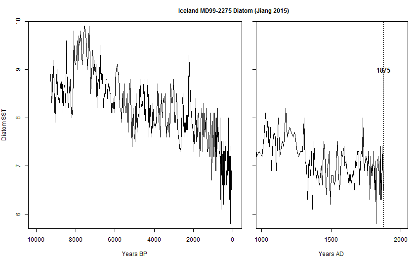
The decrease in summer temperatures is not surprising at all. It has been going on for a very long time and it is probably due to the effect of falling obliquity on ocean temperatures.
This is a biological (summer) diatom proxy from Icelandic waters MD99-2275. It pretty much sums what is going on up North. Although a secondary trend upwards is possible for some time, the primary trend is down, down, down.
Source: Climate Audit from Jiang et al., 2015.
If low solar activity had much of an influence on global temperatures, we wouldn’t have seen the big rise in temperatures last year, and the expected additional rise this year, no?
Unless, as David Evans hypothesizes, there is a significant time delay on the order of one sunspot cycle.
Yes there is very little correlation on temperatures and solar activity on the short term, but the correlation improves the longer the timeframe considered and it is quite good already at the multidecadal level.
the correlation between declining solar polar field strength and temperature is clearly demonstrated by the character of results on minima as shown above, i.e. like parabola
you can also look at maxima on stations with good records from the past, i.e.
http://oi60.tinypic.com/2d7ja79.jpg
Based on 35 years of satellite data.
Actual TSI measured during years between sunspot peaks is about 1361 watts per square meter.
Actual TSI measured during years of higher sunspot activity is about 1361.5 watts per square meter.
Those years with higher sunspot numbers are a little more variable with short times of 1362 watts per square meter. The 2014 paper by Kopp shows the acual data.
http://www.swsc-journal.org/articles/swsc/abs/2014/01/swsc130036/swsc130036.html
The amount of solar variability in terms of solar energy reaching Earth is very low, even in historical terms, but TSI before satellites is less certain. No one really knows TSI during the Maunder minimum, or earlier.
Land Northern Hemisphere in total (40% land) and the global Land only temperatures show clear presence of the solar Hale cycle periodic component.
http://www.vukcevic.talktalk.net/5Spectra.gif
Since science has no explanation for this phenomenon it doesn’t mean that it doesn’t exist.
Vuc, statistics science (the study of statistical methods) does indeed have an explanation for the graph you have posted. Have you explored that?
He can’t get past the feeling he gets from his brains pattern detection systems. He is not yet at peace with the reality that our brains seek out and perceive patterns, even where none exist, and that squinting harder when looking at the graphs, instead of using statistical analysis, is not the answer.
Statistics is not a science, it is an art in crafting a ‘numerical origami’; its worth is residing in the mind of the beholder.
I hope your science is a bit more sound than your name spelling ability. good bye !
Mr. Schaeffer , it is so kind of you to explain my emotions and cerebral functionality so concisely; I could have lived rest of my life in a total ignorance of my character.
On the matter of science, it goes without much elaboration that if something has a clear physical explanation the use of statistics is surplus to requirements. On the other hand in the absence of a clear physical explanation ‘theorylogists’ resort to statistics, which “can prove almost anything but the truth”.
Without any intention whatsoever in delving into your personal emotional and other attributes I wish a good day to you sir.
The history of statistical science has been chronicled. It is not an art but a legitimate area of research, often using random data to test the strengths and weaknesses of standard and proposed statistical methods. Something as complex as climate demands its use. Why? Most often the issue is that while x appears to be related to y, it is actually a confounding factor z that connects them (think CO2 and long term rise in global temperature – a good case of missing the confounding factor). A close second in climate science is the overly re-worked data making an elephant’s trunk tie itself into knots. Or loop up and down in graceful arcs.
We already have some evidence of the link between low sun spots and climate from 2009. It was a year in which regional temps (NH) were lowered and the mechanism was also revealed. It came from lack of weakening of the jet stream in summer and unseasonably cool months. So, one year (season) and regional impact does not make a global climate impact for models but it is marked as a likely pattern to watch for in an extended solar minimum over several years of that 2009 experience. Throw on top of that the El Nino decline and AMO multidecade decline and it could get interesting, if not confusing. I’m sure the models will sort it out. sarc
The sun is as “smooth” as a billiard ball.
“Smooth” refers to the topographic texture. “Blank” means it is featureless, like the uniform color of a billiard ball. I believe that David’s choice of words was better than yours.
Let’s do this from the bottom up. I am going to dismiss atmospheric heating by the Sun because on a daily basis, we turn away from the Sun and rather rapidly cool off, all things being equal. Air does not store heat. Since I believe the oceans are the source of heat, stored up and released in swings of various degrees and lengths of time, let’s do some calculations:
The “Specific Heat” property says that water requires 1 calorie for each gram of water present and each degree Celsius that those grams of water heat up. Other materials require a different amount of calories to heat up.
Since it takes 1 calorie to heat a gram of water 1 degree Celsius, and 1 Joule per second (which is also 1 watt) is equal to 0.238902957619 calories, we now know that it takes 4.184 J/s to heat one gram of water 1 degrees Celsius. To expand, 4.184 joule of heat energy (or one calorie) is required to raise the temperature of a unit weight (1 g) of water from 0 degrees C to 1 degree C, or from 32 degrees F to 33.8 degrees F. Now consider the volume of ocean. Granted, ocean water is not pure water, but the exercise will work for illustrative purposes. So consider the volume of ocean. There are 3785.4118 grams of water in a gallon of the stuff. It takes 15,838.163 J/s to heat that gallon by 1 degree. That’s 15,838 Watts consumed to heat that water 1 stinkin degree. The link below will fill you in on how much heat is currently estimated to be stored in the oceans. For those of you who wish to use the British Thermal Unit: 1 Btu (British thermal unit) = 1055.06 J though for the life of me I don’t know why anyone would ever use that awful calculation. Unless you have a caveman sized grill and like to say big numbers followed by BTU. Anyway, it must be clear to you by now that the tiny amount of VARIATION in solar metrics the solar enthusiasts are putting forth has the energy to do anything at all measurable let alone observable to climate via transfer of energy from the top of the atmosphere to its surface and below is just not plausible. Not even when somehow amplified.
http://www.nodc.noaa.gov/OC5/3M_HEAT_CONTENT/
I’m afraid nobody will read your excellent comment, and if by exception anyone did, s/he would understand what you are so accurately underlining.
What about a graphical comparison, Pamela?
I am terrible at creating graphs I can post. Don’t know how to go from Excel to a picture to an embedded comment. Besides, the scale would have to be reduced to the degree that at least one bar on the graph would not be visible and the other one would not fit on the page.
I did read her long missive and I’m afraid I missed the point she was trying to make. I’m not sure the problem was mine because I don’t encounter the problem very often.
(shades of gray…)
I don’t suppose that if the delta were cumulative it would make any difference. I never did care for integration anyway.
Are you suggesting that the oceans are the ultimate source of heat? Or are you just ignoring the fact that when warm air passes over water it evaporates some of that water and then transports that water vapor with its latent heat to some other place in the atmosphere?
BTW rocks store heat. That is one of the reasons we have an UHI effect.
The oceans store and release absorbed solar energy.
“The oceans store and release absorbed solar energy.”
As do the land masses. Its just that the land rises to higher temperatures for the same insolation and releases the solar energy more quickly. Water vapor also stores and transports solar energy. Your Point?
However, the oceans can only release the absorbed solar energy if the atmosphere is colder than the water. Where are you going with this.?
This diagram sums up the ocean and atmosphere. Where I disagree, I do see science that the sun contributes quite a bit towards temperature during numerous cycles. The time scale I estimate is roughly two and half cycles until the planet reaches equilibrium with a constant change in solar activity, say 0.5 W/m2 at the surface.
http://i772.photobucket.com/albums/yy8/SciMattG/atmosphere-vs-ocean-heat-capacity2_zpsjjwuhpbk.jpg
Specific heat is the amount of energy that raises one kilogram of matter by 1 Kelvin.
For seawater, specific heat is 4000 Joules per kilogram.
For air, specific heat is 1000 Joules per kilogram.
On a volume basis, seawater has 800 times the density of the atmosphere above the surface. So, for equal volumes, the ocean surface has 3200 times the heat capacity of the atmosphere.
Also, the ocean absorbs and thermalizes almost all solar energy, it has a very low albedo.
Rocks have a greater density than water, but have lower specific heat capacity.
So on a global basis, yes the sun heats the oceans, and the oceans then heat the atmosphere.
Just compare the annual temperature variance of Hawaii or Guam to any central continental weather station.
Acceptable for a first-order approximation. However, there are some things to consider. You left out the latent heat of water vapor in the air. Also, while the reflectivity of water is very low when the sun is directly overhead, and even with angles of incidence up to about 60 deg, the reflectivity approaches 100% at glancing angles, i.e. the limbs of Earth have very high reflectivity.
Very nicely put, except for going from grams to gallons.
I did that for those of us who buy milk by the half gallon and spray weeds with a 3-gallon capacity backpack sprayer. It is something that is very familiar to a farm girl in NE Oregon and to the rest of the US. Which explains the BTU mention. It’s apparently a guy thing, kinda like a mancave.
You must love it when you need a new air conditioner and they start talking about tons, Pamela.
Do you know why AC is measured in tons?
Haven’t the foggiest.
No one has and no one will be changing his/her opinion. The only way it could change is if the data supports one way or another the opinions that are out there.
The data going forward will go a long way in proving who is correct and who is not correct.
Salvatore, no. The data will not go a long way to proving your thesis. You must develop a reasonable series of mechanisms, and then put those to test. Start with a literature review. Uh oh. So far, the literature is rather thin regarding your thesis. For everyone you may find that supports your mechanisms, there are multiple ones that say the opposite. You have a very rough road ahead.
Pam what do you think me and others have been reporting all these months . I listed many mechanisms on my post sent june 30 12:16 pm.
You choose not to believe them . Again I want to see if the climate responds to my low average value solar parameters if it does you and the ones that agree with you will have to explain and prove why it is not correct .
The oceans are what help to keep our temperatures relatively stable. But they are not the driver. I know you want to believe that, but it is purely wishful thinking on your part. Give it a rest.
Salvatore, if you’re shown to be in the right, nobody’s going to stick around to prove nuthin’! AGW will be over, anthony will take up golf, and the rest of us will have to find another hobbie… (☺)
No, I think the warmistas will simply find a new way to torture us, or at least try.
Until they are all hogtied in a dungeon somewhere.
( Hey, that was a joke, for all the hate miners.)
Was hoping to hear some news on this, but nothing further yet…. it would certainly help with some of the above questions/answers.
http://www.nasa.gov/feature/goddard/saving-nasas-stereo-b-the-189-million-mile-road-to-recovery
Oh deary me.
Since AGW is faith based let’s all convert to group mindlessness. Works on the crime rate.
Leif,
Very off topic but I’m interested in your take on this question I have asked the ligo folks:
Since time theoretically stops at the singularity (or the event horizon depending upon whom one listens to), in our reference frame as the observer, how can we ever measure or detect something that should take an eternity, again from our reference frame, to play out? Or posing the question another way, where in the spiral inward in the merger does the large spike in the gravitational wave get generated and how can we ever know given the relativistic time dilation effects of the high gravities involved even before the “merger”? From our reference frame, as the observers, all of this should take a very, very, very, long time and the actual merger an infinitely long time.
The simplest answer is that what we have observed is just what is predicted by General Relativity. To get an intuitive feeling for what is going on is very hard, as our experience does not cover the situation.
Leif,
Thanks for your response.
Jim
Time never stops. The relativity of such does. Just sayin…..
Ossqss,
Depends upon your reference frame. For an observer in our frame of reference, time stops at the black hole per GR. For the two black holes, in their frame of reference, they merge. However, we could never observe it from our frame of reference, per GR. A conundrum of high order.
Like I said.
Mimsy Were the Borogoves…
Postmodern astrology.
AF,
I’m looking at the graph of the spike in the ligo observation of the subject gravitational wave and thinking that GR says we could never observe that from here. Mimsy, indeed.
Or best theory says infinity.
Reality says otherwise.
What does that tell you about our best theory?
How do you know what reality is?
One answer is that reality is what we measure. Our theories are shorthand expressions for all the measurements we have ever made. So far we know of no measurements contradicting our theories. when we find such, we extend or change the theory to match.
Leif,
The fact that we can make the subject ligo observation from our reference frame, so we say, violates the GR theory we are assisting in validating with that observation. This “measurement” is in conflict with our theory or it is incorrect.
The LIGO observers don’t think so.
Leif,
I’m reading a book called Biocentrism by Bob Berman and Robert Lanza, MD, which you might find interesting. Perhaps we create reality by observing and taking our measurements. It’s about issues like how we collapse the probability distribution wave function of a particle when we observe it. You should read at least the first few chapters. Not sure it has any answers but it sure brings the questions into sharper focus.
Perhaps the wave function never collapses, but instead the universe splits into two:
https://en.wikipedia.org/wiki/Many-worlds_interpretation
Have not yet read enough of the Biocentrism but we, our consciousness, would still seem to be the causal factor, be it wave fuction collapse or split of time line or universe. Multiple universe or string theory, or multiple dimensions or “many worlds” theory seems to avoid ability to observe and measure in that “other place”.
Amazing what happens when you study the weather:
it all works like a clock and it seems all parts of the clock sit inside the sun….
Must be that somebody carefully designed it?
HP,
For me, intelligent design is beyond question. All else is vanity. For every answer we find there are several more questions which arise. Keeps us on our toes.
I am a counter example to intelligent design. If I am the best she could do, she is not very good at it.
thanks, Jim. God bless you.
Leif,
The older I get the more I would agree and those few friends I have that are older than I am tell me it only gets worse.
Let’s not ignore implications from land use changes.
Terrestrially 47% but is that good data?
The chaotic nature of solar activity
http://papers.ssrn.com/sol3/papers.cfm?abstract_id=2767274
interesting. I also found some inconsistencies in the SSN records that made me suspicious…. SSN is a subjective measurement and it is better to look at the solar polar magnetic field strengths.
The SSN [or even better the Group Number] is a VERY good measure of solar activity. The polar field is a VERY good predictor of the SSN, but only goes back a few cycles, and is not a measure of what hits the Earth. For long-term work, the SSN is the measure to use. To see how well the SSN matches the magnetic field of the Sun check out http://www.leif.org/research/SSN/Stenflo.pdf “the average unsigned vertical magnetic flux density has a remarkably tight correlation with the sunspot number”.
Often, people disparage the SSN because it does not match their pet theory. Don’t be one of those people.
Hi Leif
I quote from the paper you quote to me:
“SSN is an index with considerable subjectivity, depending on manual
determinations with small telescopes,”
eye strength and magnification probably being the main factors of subjectivity.
I rest my case. I will go along with it for about 90 years back, but that is it.
Before that, everything becomes murky, just like the temperature record before the 1950s….
One overcomes the subjectivity by scaling the observers to a standard observer. In this way an objective measure is obtained, where the scaled values from different people closely agree.
If you rest your case, you just become of of those people I referred to who don’t like the SSN because it does not match their pet theory. There are [sadly] many such people, so you are not alone, but that does not make you reasonable or right.
HenryP,
No measurement, and especially no series of measurements, is without error. Estimating the total area of sunspots is more subjective than counting the number. There is good agreement between different SSN observers over time, which should give one confidence that they are reliable. Because the means to measure polar field strengths did not exist before modern times, if one wants to try to estimate their past values, then some proxy has to be found. It seems that SSNs make a good proxy. Sometimes less than ideal measurements must be relied upon when trying to explain things. That is particularly true for trying to reconstruct changes in the past. And, sometimes that is absolutely essential when phenomena change periodically over a span of time that is greater than a single human’s adult lifespan. It is better to try to understand the nature of the deficiency of past measurements and correct for them, if possible, than to discard them entirely.
that is another problem with spot counting
the difference in intensity?
Henry,
There is no ‘difficulty’. When normalized to a common standard, observers agree on the SSN, and we find that the SSN is a good proxy for the magnetic field, the Total Solar Irradiance, the microwave flux, the cosmic ray flux, the geomagnetic variations, and just about any other index you might come up with.
dear Leif
I only observe my own test results, compile and evaluate. I postulate. Where other people’s results agree with mine they must be right/
where other people’s results disagree, with mine, they must be wrong.
that must be in our nature.
Anyway, it seems you did not challenge me too much anymore on the existence and reality of the Gleissberg cycle affecting the global weather (causing 43 yrs warming and 43 yrs cooling) so it seems we are moving closer together.
Anyway, it seems you did not challenge me too much anymore on the existence and reality of the Gleissberg cycle affecting the global weather
Not every silly idea is worth a challenge…
tables II and III http://virtualacademia.com/pdf/cli267_293.pdf
quite silly actually for you to ignore the overwhelming evidence
“The easiest one to fool is yourself” Richard Feynman
you must be getting old, talking to yourself a lot now, are you?
anyway, you heard God’s voice again inviting you to the party beyond life. He is still calling you. Best wishes.
God? she has no impact on me, and her shouting does not really belong in any scientific debate. Of course, if you are not doing science, perhaps she can be your guiding light.
May I complain again about how cold it is here in Brisbane?
Well, I’m going to, anyway.
It’s chilly here. Could someone turn the sun up a bit, please?
Heat comes from bodies of water. Jump in the tub! Turn out the light and see if the water gets cold. Report results to P. Grey.
Yep. And in a hurry. Most tubs are not made for a Calgon appointment with the tub. Water gets too cold before I would wish. By the way, you forgot the “light the candle” after you turn out the light.
(Insert previous Max Photon comment here)
If solar activity has no measurable effects on climate, why is there a strong repetitive correlation throughout history?
It must have an effect. We just don’t know how.