Guest Post by Willis Eschenbach
I’ve been mulling over a comment made by Steven Mosher. I don’t have the exact quote, so he’s welcome to correct any errors. As I understood it, he said that much of the variation in temperatures around the planet can be explained by a combination of elevation and latitude. He described this as a “temperature field”, because at any given latitude and elevation it has a corresponding estimated temperature value.
Intrigued by this idea, I decided to use the CERES dataset. However, rather than using latitude, I decided to take a look at how well a combination of the sunlight and the elevation can predict the average temperature. Let’s start with the average surface temperature. It’s shown below in Figure 1.
 Figure 1. Average surface temperature according to the CERES dataset, on a 1°x1° gridcell basis.
To estimate the temperature, what I did was to make a simple linear function of solar energy and elevation (see end notes for details). This gave me the following estimate of gridcell temperatures.
 Figure 2. Estimated surface temperature based on elevation and sunlight. R^2 = 0.94, p-value less than 2e-16. See end notes for calculation.
Now, that’s a pretty good facsimile of the actual temperatures shown in Figure 1. Indeed, the “R-squared” (R^2) of the temperature field and the observations is 0.95, meaning that the temperature field explains 95% of the variation in the observed temperature.
That’s not the interesting part, however. The fun questions are, where is the temperature NOT as expected, and why? Where is the greatest departure from the estimated temperature, and why is it there? To investigate those, I next looked at the difference between observations and the estimated temperature field. Figures 3 and 4 show two views of the observations minus the temperature field.
 Figure 3. Observed temperatures minus the estimated temperature field, centered on Greenwich. Gray line shows the boundary between positive and negative values. Positive values (yellow to red) mean that the observations are warmer than expected.
I found this most fascinating, as it shows the great oceanic heat transport systems that move the energy from the tropics, where there is an excess, to the poles where it is radiated to space. I was surprised to see that the warmest location compared to expectations is the area above Scandinavia. This has to be a result of the Gulf Stream current which is also quite visible along the edge of the East Coast of North America.
I note that as we’d expect, the deserts and arid areas of the world like the Sahara, the Namib, and the Australian deserts are warmer than would be otherwise expected.
You can see another view showing the overall results of the El Nino/La Nina heat pump below in Figure 4. This is the same data as in Figure 3, but centered on the Pacific.
 Figure 4. Observed temperatures minus the estimated temperature field, centered on the International Dateline. Gray line shows the boundary between positive and negative values. Positive values mean that the observations are warmer than expected.
Here we can see the area off of Peru that runs cool because the El Nino/La Nina pump pushes warm surface water across the Pacific. This exposes underlying cooler waters. When the warm water hits the Asia/Indonesia/Australia landmasses, the warm water splits north and south and moves polewards. As with the area above Scandinavia, the heat seems to pile up at the polar extremities of the heat transport system. In the case of the Pacific, the northern branch ends up in the Gulf of Alaska. The southern branch ends up where it is blocked by the shallow narrows between the Antarctic Peninsula and the tip of South America.
In any case, that’s what I learned from my wanderings. The beauty of climate is that there are always more puzzles to be solved and oddities to be pondered. For example, why are the western parts of the northern hemisphere continents warmer than the eastern parts?
My best to each of you,
w.
As I’ve Mentioned: If you disagree with someone, please quote the exact words you disagree with so we can all understand your objections.
The Math: I used the form:
Estimated Temperature = a * sunlight + b * elevation + c * sunlight * elevation + m
where a, b, c, and m are fitted constants. The results were as follows:
Coefficients:
Estimate Std. Error t value Pr(>|t|)
(Intercept) -4.052e+01 7.122e-02 -568.9 <2e-16 ***
sunvec 1.675e-01 2.033e-04 823.8 <2e-16 ***
elvec -1.918e-02 7.723e-05 -248.4 <2e-16 ***
sunvec:elvec 4.354e-05 2.485e-07 175.2 <2e-16 ***
---
Signif. codes: 0 ‘***’ 0.001 ‘**’ 0.01 ‘*’ 0.05 ‘.’ 0.1 ‘ ’ 1
Residual standard error: 0.2557 on 64796 degrees of freedom
Multiple R-squared: 0.9479, Adjusted R-squared: 0.9479
F-statistic: 3.933e+05 on 3 and 64796 DF, p-value: < 2.2e-16
where “sunvec” is average gridcell solar energy in W/m2, and elvec is the average gridcell elevation in meters.
Thanks, Willis. Your figures 3 and 4 are very interesting.
Given some of the statistical analyses I’ve seen in climate research, the R^2 you got is just amazing (and I mean that in a good way). One question I have is the differences you got in the US from the Rockies to the midwest and east. I’m curious as to whether the zero error line runs along a given altitude. It’s east of the Rockies and it’s hard to make out exactly where it lies. You equation is linear, but could there be a polynomial term or terms? If the differences in the Rockies, for example, were due to Pacific Ocean I would assume that the effect would not extend all the way to the plains, but stop to the west of the Continental divide.
The thing to understand is that the warming occurs on the lee side of the mountain range. This is not warm are being “blocked” as a number of commenters mistakenly think.
Look up Foehn wind, it happens all over the world. In the Rockies it’s called Chinook.
It is also the reason for the warming on the Antarctic peninsula that Steig et al incompetently managed to mangle into being a continent wide effect.
Has Willis discovered the missing ‘hotspot’. Its on its Scandinavian holidays….. /sarc
We can see the pattern of Willis’ map is a reflection of the persistent ocean currents that are driven primarily by the Coriolis force.
http://upload.wikimedia.org/wikipedia/commons/1/1f/North_Pacific_Subtropical_Convergence_Zone.jpg
Also the warm water that gets up around Scotland and Norway has no way out. So this is not just a surface current.
http://commons.wikimedia.org/wiki/File:North_Atlantic_Gyre.png
This water becomes more saline and thus denser to evaporation. It then sinks in the Arctic, forming an important part of the thermohaline circulation.
It is easy to see from all this discussion that long period changes in the magnitude of these ocean currents will lead to warming or cooling “trends” in global averages.
Oops, seem to have lost my N. Atl map
http://commons.wikimedia.org/wiki/File:North_Atlantic_Gyre.png
“It is easy to see from all this discussion that long period changes in the magnitude of these ocean currents will lead to warming or cooling “trends” in global averages.”
And it does show up as regional swings in minimum temp. It might also show up in the magnitude of maximum temp, but max temp has no change in annual averaged derivative, where min temp shows large changes.
http://upload.wikimedia.org/wikipedia/commons/b/b4/North_Atlantic_Gyre.png
WP seems to filtering out the link for some reason. Try again.
The arid zones (eg much of Autralia, except the humid east and north coasts) show positive temperature anomalies (ref fig 3). It would seem that lower humidity (decreased thermal capacity) has a greater effect increasing temperatures, than does the increased greenhouse effect from higher humidity (increased thermal capacity), as the humid tropics all show negative anomalies.
There also looks to be a warming Foehn Effect in the mid-latitudes of North and South America.
Steven Mosher May 15, 2015 at 8:59 am
Thanks, Mosh. And thank you for your long and detailed comment. I’m glad the loquacious Mosh showed up and not the cryptic comment Mosh.
I understand your distinction, all but the last part. You say that the climate of a location is what is determined by the physical properties of the location. And weather is the difference between observations and climate.
The part I don’t understand about this is the comment that “climate change is in the weather field”. Given that T = C + W, for a given T, if C changes (“climate change”) then W has to change as well. Is that what you mean by “climate change is in the weather field”? Or are you saying that C is constant, so any change will be found in the weather field? If so, what evidence do you have that C is constant?
In the link you provide just above, you say:
The issue I have is that your “spatially focused” formulation also changes with changing time. For example, we get a good fit with just elevation and latitude in the simplest formula, viz
temperature = a * cos(latitude) + b * elevation + intercept
where a, b, and intercept are constants.
The problem is that if we use different time periods, we get different values for a, b, and intercept. Here’s an example. I divided the CERES data in half and re-calculated the best-fit constants for the first half and the last half of the data.
> lamod=lm(firsttvec~latvec+elvec,weights=as.vector(latmatrix));round(lamod$coef,3)
(Intercept)      latvec       elvec
    -31.347      60.712      -0.006
> lamod=lm(lasttvec~latvec+elvec,weights=as.vector(latmatrix));round(lamod$coef,3)
(Intercept)      latvec       elvec
    -30.391      59.623      -0.006
As you can see, while the rate of change of the temperature with elevation (the lapse rate) is pretty stable, the change in temperature per degree of latitude and the intercept are different between the two periods. Now that difference might just be noise … or as is more likely, the system is not stationary. And if the system is not stationary, then just what is meant by “climate change”?
In any case, the concept of using a temperature field is a most interesting one, and one which leads to a variety of valuable insights.
My best to you, and thanks again for your valuable comments.
w.
“As you can see, while the rate of change of the temperature with elevation (the lapse rate) is pretty stable, the change in temperature per degree of latitude and the intercept are different between the two periods. Now that difference might just be noise … or as is more likely, the system is not stationary. And if the system is not stationary, then just what is meant by “climate change”?”
Exactly. The system isn’t static.
“The part I don’t understand about this is the comment that “climate change is in the weather field”. Given that T = C + W, for a given T, if C changes (“climate change”) then W has to change as well. Is that what you mean by “climate change is in the weather field”? Or are you saying that C is constant, so any change will be found in the weather field? If so, what evidence do you have that C is constant?”
C is constant by construction. latitude and elevation dont change as a function of time. The regression is done to simultaneously remove latitude and elevation and seasonality from the temperature.
This becomes the “geographic climate” . lets say for example that the lapse rate at a location changes over time. The average lapse rate end up in the climate field, any changes over time ( like those caused by climate change) end up in the weather field. So what you see is that changes in climate ( deviations from
the geographic climate) end up in the weather field. climate is the thing that doesnt change. Its what you expect.
Now you can of course divide the data into separate piles based on time and see that the coefs change.
All you’ve done there is put climate change in different piles.
I suppose you could use a base period 1950-1980, calculate the geographic climate for that period and then all the climate change from that base period would get tossed into the residual.
If the question is ‘ is C always constant?” is it constant before 1750 when our data starts?
A) probably not.
B) get more data from before 1750 and we can test.
C) It’s not important since we are are interested in climate change relative to the period of record.
I like the description of T=C+W from Mosher. I am sure it can be developed.
I can understand how he tries to justify infilling.
However, if we were to agree that T=C+W and there is a ‘temperature field’ does that not lead towards just one very well placed temperature sensor per continent?
Seven sensors, perfectly sited and maintained, streaming data to the world?
You could even have a competition for the location of each sensor (or choice of, if already in place).
The temperature field will inform us what constant to apply to each sensors output.
Job done.
you can derive the minimum number of stations required. its on the order of 60 perfectly placed stations
(Shen)
seven sensors would not work because lapse rate is contingent upon temperature as Willis notes.
so you need sampling across latitudes. it need not be uniform,
you need sampling across altitudes— high altitude ( top of everest ect) are lacking..
ideally you would have sampling from all land classes.. some land classes are collinear with land class and altitude
( like permanent ice)
Suffice it to say when 90+ percent of your variable of interest is determined by lat and elevation you are Nibbling at the edges.
To give you an example.. I tried to ad albedo to the regression. it was a huge amount of work and R^2 didnt budge . The Errors get spatially re arranged, your local fidelity improves.. but the global answer dont change much. I tried adding terrain slope and aspect ( north facing) Huge amount of processing.. also r^2 didnt move.. but local changes would occur. Im playing with some other things… lots of work and failure.
In the end the more you add to the regression the fewer adjustments you would see with our method, local values would shift around.. local accuracy would improve… but the global answer simply will not budge.
The warming you see in the global average is there to stay. better to move on and tackle other questions.
For technical considerations its fun to improve the local fidelity.. but not of interest to the greater questions of climate science.
“The warming you see in the global average is there to stay. better to move on and tackle other questions.”
Which is why I’ve gone on to look at the annual rate of change, there isn’t a “residual” in the annual change in max temp, but it could reach its limit earlier and stay longer, there is a change in the rate, but it also looks like it could have peaked, and is changing direction, as well as there is a big swing in the “residual” on min temp. How much of these are the BEST trend, and isn’t there more clarification of your output?
It feels much like deception by leaving important facts out.
How much is just warm water moving around, since much of the derivative of min temp is not global, it seems like much isn’t from Co2, as well as nightly cooling exceeding prior day’s warming. Either the surface as already reached equalibrium or the warming is from another source( like the oceans).
And I think cooling >warming is a powerful example of proof that is accessible to everyone.
BEST, could lead the way to better understanding, but. ……….
micro.
go publish or pick a better tree to bark up
Mosh, thank you.
Willis I am looking at your figure 4 and see that it averages data from 14 years, The average duration of an ENSO cycle is 4 to 5 years which means that three ENSO cycles have been telescoped into this graph. The El Nino and La Nina phases of ENSO are substantially different but the average shown is basically that of f only the La Nina phase. La Nina, unlike the El Nino phase, is spread out over the ocean and that is what we see. To catch the El Nino phase in action, you should look at the data with at least one year resolution, not 14 years as here.
Willis and Steve: I helped my son regress average temperature data for US cities versus latitude, longitude and elevation and found a remarkable fit using just latitude and elevation. We even got the correct lapse rate. (I can’t tell if Willis did from his post.) The only location which deviated was the Pacific Northwest, which was too warm.
The regression also allowed me to convert degrees of global warming (a meaningless number to most people) into distance moved south (a more meaningful concept for some). 1 degC of warming in the US is equivalent to moving south 100 miles. AGW usually doesn’t sound so awful when expressed in terms of distance. However, the width of the corn belt in Iowa is about 200 miles. Global warming equivalent to moving 200 miles south certainly will require corn farmer to adapt.
Yup. Great to see a dad helping his kids..!!!
“why are the western parts of the northern hemisphere continents warmer than the eastern parts?”
Because the land on the eastern side is moving towards the cold night-time temperatures.
Because the land on the
eastern side is moving
towards the cold night-time
temperatures.
____
hm, no – in this context every discrete location isn’t east or west, it just ‘rolls’ in 24 h to east, steadily changing its ‘orientation’ to the sun.
Regards – Hans
“why are the western parts of the northern hemisphere
continents warmer than the
eastern parts?”
Because the land on the
eastern side is moving
towards the cold night-time
temperatures.
____
in this context there is no absolute east/west binding.
Any discrete location is just ‘rolling’ 24 hours to the east, changing its relative position to th sun.
Regards – Hans
A physics point that someone may be able to help me with:
The answer will have relevance to the concept of a temperature field as defined by Willis and / or Mosher thus:
“much of the variation in temperatures around the planet can be explained by a combination of elevation and latitude. He described this as a “temperature field”, because at any given latitude and elevation it has a corresponding estimated temperature value”.
If a single CO2 molecule is floating in an atmosphere of Nitrogen at a height of, say, 1000 metres, does it ‘see’ the surface below at a temperature of 288k or does it see a lower surface temperature after conduction and convection has taken a slice of the surface kinetic energy out between the surface and its position at 1000 metres?
or to put it another way:
Does the radiative flux from surface kinetic energy at 288k actually get received by such a molecule or does it receive a portion of that 288k by radiation and another portion by conduction and convection so that the radiative portion is a lower figure which remains as kinetic energy proportionate to height whereas the rest is from conduction and convection and is in the form of potential energy which is not heat and does not radiate?
That CO2 molecule will have the same total energy (KE + PE) at both surface and 1000 metres and will be at the same ambient temperature as its Nitrogen surroundings.
If one then places it at 2000 metres it would presumably receive proportionately less KE from surface radiation and more PE from conduction and convection would it not?
Does the mass of a radiatively inert atmosphere ‘take out’ a portion of the radiative flux progressively with height by means of conduction and convection?
“If a single CO2 molecule is floating in an atmosphere of Nitrogen at a height of, say, 1000 metres, does it ‘see’ the surface below at a temperature of 288k or does it see a lower surface temperature after conduction and convection has taken a slice of the surface kinetic energy out between the surface and its position at 1000 metres?”
In dry nitrogen, it should only see the surface, but at that BB temp, it will most likely only see the 15u wavelength, there will be some probably of a capture. At 2000m the 15u flux will be lower, so the probability will decrease for any single photon. But as long as the flux is high enough, and it’s not already captured a photon or has given the captured energy to another atom, it will quickly capture another 15u photon.
It will always have the possibility of exchanging KE, with nearby nitrogen atoms (molecules ?).
Yes, I can see that the CO2 molecule would adsorb radiation at 15u since that is the missing wavelength at the top of the atmosphere when CO2 is present.
The question is whether it would absorb an amount of 15u commensurate with a surface temperature of 288k or whether it would receive it at 278k which is the ambient temperature at 1000 metres due to the Dry Adiabatic Lapse Rate slope reducing temperature by 10K per 1000 metres.
The Nitrogen at the surface achieves 288k purely by conduction from the surface yet is 278k at 1000 metres as a result of upward convection causing decompression.
If the CO2 molecule is also 278k at 1000 metres it is presumably getting that kinetic energy from the surface but the internal energy of the molecule (KE + PE) is the same as the Nitrogen i.e. KE of 278k and PE of 10k.
So at 1000 metres one has KE of 278k and PE of 10k for both CO2 and Nitrogen.
At 2000 metres one has KE of 268K and PE of 20K and so on.
So one could argue that the CO2 molecule at 1000 metres is only seeing 15u emanating from the surface at a temperature of 278k and not 288k. At 2000 metres it would be 268k.
It seems that the CO2 molecule sees a reducing radiation flux proportionate to its height and at top of atmosphere it would be down to 255K.
The explanation would seem to be that conduction and convection takes out a proportion of the radiative flux related to height. It would do so at all wavelengths emitted from the surface, not just at 15u. Thus only 255k escapes to space after conduction and convection have taken a bite out of the radiative flux from the surface.
The ultimate fate of the 15u absorbed by the CO2 molecule is a separate issue.
Does conduction and convection reduce the radiative flux from surface to top of atmosphere or doesn’t it?
At those surface temps, it mostly sees only 15u (as the flux is pretty large ) but 15u has the equivalent temp of ~193K, Co2 also has an absorption band at iirc 4u, which is like 600 or 800F, so there little flux at 288K.
It’s all about absorption and flux.
So for a CO2 molecule at 1000 metres how much of its kinetic energy (commensurate with a temperature of 278k) comes from radiative absorption from the surface at 288K and how much comes from conduction and convection?
One assumes the potential energy content is all a matter of conduction and convection so what I wish to know is why it only acquires 278k of kinetic energy if it is receiving radiation from a surface at 288K.
Does it see a surface at 288k or at 278k? If the former then why is it only at 278k?
A Co2 molecule can’t “see”, either temp, the flux rate is slightly different at 15u though.
If a CO2 molecule is 278k 1000 metres above a surface at 288k why is it colder than the surface which is radiating towards it at 288k?
What happens to that 10k of IR between surface and molecule?
Co2 doesn’t notice or care about the difference in IR. If there is a difference in temp it’s due to KE exchange with the nitrogen.
Well yes, but that is my point.
The tmperature decline is caused by KE exchange with Nitrogen between surface and 1000 metres.
That KE exchange is conduction.
So conduction takes out 10K of IR flux betweeen surface and 1000 metres.
The CO2 molecule is heated to only 278k by radiation from the surface at 288k.
The other 10k has been processed by conduction and convective uplift and is still present in the molecule but as potential energy which is not heat and does not radiate.
Mass does block the IR flux via conductive absorption and subsequent convection.
It is therefore mass which reduces the IR flow to space to 255k from a surface at 288k and not back radiation.
“The CO2 molecule is heated to only 278k by radiation from the surface at 288k.
The other 10k has been processed by conduction and convective uplift and is still present in the molecule but as potential energy which is not heat and does not radiate.
Mass does block the IR flux via conductive absorption and subsequent convection.
It is therefore mass which reduces the IR flow to space to 255k from a surface at 288k and not back radiation.”
Maybe I don’t understand you, but if I do, no.
A single CO2 molecule can capture a 15u photon, and either through a collision with the nitrogen give some of that KE away, or it can emit a 15u photon giving that energy away.
It can also through a collisions be whatever temp the nitrogen is, and it should still be able to capture and then emit a 15u photon in any direction. An antenna can capture a specific wavelength photon, and can be at various temperatures, I think they are totally separate processes. In Co2 there is likely some possibly of the energy getting converted to heat or being emitted, but I would suspect that it works both ways, ie KE can also be captured then emitted as a 15u photon, if it has the correct bending motion.
micro said:
“A single CO2 molecule can capture a 15u photon, and either through a collision with the nitrogen give some of that KE away, or it can emit a 15u photon giving that energy away.
It can also through a collisions be whatever temp the nitrogen is, and it should still be able to capture and then emit a 15u photon in any direction”
Well I’m glad you said it can EITHER lose it by collision OR by emitting a photon. Most contributors here seem to think it can do both with the same package of energy at one and the same time.
The single absorbing CO2 molecule can also do something else.
If it is already at the temperature of adjacent Nitrogen (as would be the normal case) and then absorbs a 15u photon from below then it will be too warm for its temperature along the lapse rate slope and will rise upward with the surplus energy converting to PE which cannot radiate or conduct away.
Have a look at the concept of hydrostatic balance within an atmosphere which is the point where the upward pressure gradient force exactly offsets the downward gravitational force.
If one adds that photon then the pressure gradient force becomes larger than the gravitational force and the molecule must rise.
Since the extra photon becomes PE it effectively disappears from sensor view, circulates through the convective overturning cycle and then reappears as KE again at the bottom of the nearest descending column.
In rising it enhanced convective ascent from within the atmosphere, not from the surface so it cools the surface a fraction and then rewarms the surface again when it appears at the other end of the convective cycle.
Since it is rewarming a cooled surface it is no longer 15u but gets converted to another wavelength by the surface so that it can then escape through the atmospheric window.
What you end up with is the surface at the same temperature as before but a bit more PE was within the convective cycle whilst the energy derived from the 15u photon ran through the system and was converted to a wavelength that could escape.
The convective cycle deals with the CO2 absorption of 15u so that it does not affect temperatures and can escape to space from a different wavelength.
I think, once it’s lost some of the flexing mode energy that is from the captured 15u, it doesn’t have anyway to emit a photon at a different wavelength, and would only lose it from collisions with other molecules. Now that energy can warm some air, which can warm the ground (or interact with a water molecule), and from there can be radiated back to space at a different wavelength, but other wise i think it’s effectively trapped.
Stephen Wilde
You say of a CO2 molecule that absorbs a 15u photon
Sorry, that is wrong on at least three counts.
Firstly, an individual molecule does not have a temperature because temperature is a bulk effect of all the molecules in a volume of gas. The temperature of the volume is proportional to the RMS speed of all the molecules in the volume.
Secondly, the molecular absorbtion of photons of a gas volume does not change the temperature of the volume. The absorbed energy is internal to individual molecules: the absorbtion of a photon by a molecule alters the vibrational or rotational state of the molecule but not its speed.
Thirdly, the excited CO2 molecules in a volume of gas will not float up because the absorbtion of photons does not affect the temperature of the volume.
There is a needed caveat to the three above facts. Collisional de-excitation can provide the excitation energy of a CO2 molecule to e.g. a nitrogen molecule which it contacts. This will increase the speed of the nitrogen molecule and, therefore, collisions can warm the non-GHG molecules of a volume. Near the Earth’s surface almost all the de-excitation of CO2 molecules will be by collisions.
Richard
richardscourtney
While I know this is controversial, a single atom can have the same KE the same atom would have at temp x, it would seem to me that one could say that single atom has a “temp” of x.
This is the exception to that applies to the conversation, I don’t know what the percentage of which effect the specific atom will lose it’s energy from, maybe it’s a fraction of a percent, maybe it’s most of the Co2 depending on the pressure, actually the pressure broadening is likely the molecule losing(gaining) a bit of energy due to collision, yet still having enough energy to emit at ~15u.
Richard, I appreciate your effort to improve my terminology but I’m not sure that te points you make detract from what I am suggesting
Firstly, I only referred to a single molecule in order to try and simplify the concept. In reality there will be lots of CO2 molecules absorbing 15u, passing it on by collisions and generally accelerating upward convection as I proposed.
Secondly, changing the vibrational or rotational state can upset hydrostatice balance in order to force a change in height.
Thirdly, enough excited CO2 molecules will pass sufficient collisional energy on to enhance convection.
Thus micro’s point is correct. I am indeed applying the situation covered by your caveat.
micro said:
“I think, once it’s lost some of the flexing mode energy that is from the captured 15u, it doesn’t have anyway to emit a photon at a different wavelength, and would only lose it from collisions with other molecules. Now that energy can warm some air, which can warm the ground (or interact with a water molecule), and from there can be radiated back to space at a different wavelength, but other wise i think it’s effectively trapped”
You haven’t followed through the sequence of events I gave you.
It causes enhanced uplift which converts the former 15u into potential energy.
That potential energy cycles up and then down the convective cycle to return to the surface as KE. The surface then radiates at a range of wavelengths so that most if not all can escape to space.
The speed of convective overturning rises until the amount escaping from the surface via the atmospheric window exactly matches the 15u absorbed by the CO2.
I have no real issue with this, I just didn’t describe this part of the process 🙂
“why are the western parts of the northern hemisphere continents warmer than the eastern parts?”
Down to observed ocean currents in the northern hemisphere, where below show warm surface ones flowing the side of western continents and the cool deep ones flowing by side of eastern continents. Always since the last ice age and unlike the brief YD like events, cool deep currents never influence western sides of continents. Warm ocean surface currents never reach the eastern side of northern hemisphere continents away from the sub tropics.
http://earth.usc.edu/~stott/Catalina/images/Oceanography/surface%20currents.jpg
“He described this as a “temperature field”, because at any given latitude and elevation it has a corresponding estimated temperature value.”
Two reasons why this is not often true.
1) Temperature inversion
A temperature inversion is a thin layer of the atmosphere where the normal decrease in temperature with height switches to the temperature increasing with height. An inversion acts like a lid, keeping normal convective overturning of the atmosphere from penetrating through the inversion. This happens more frequently in high pressure zones, where the gradual sinking of air in the high pressure dome typically causes an inversion to form at the base of a sinking layer of air.
http://www.weatherquestions.com/temperature_inversion.jpg
http://www.weatherquestions.com/What_is_a_temperature_inversion.htm
2) Foehn wind
A föhn or foehn is a type of dry, warm, down-slope wind that occurs in the lee (downwind side) of a mountain range.
As a consequence of the different adiabatic lapse rates of moist and dry air, the air on the leeward slopes becomes warmer than equivalent elevations on the windward slopes.
Matt G May 17, 2015 at 9:22 am
“Not often true”? Say what? Did you notice the R^2 of ~0.94? Do you realize this means a correlation between the two datasets of 0.97?
Yes, there are a variety of process like foehn winds and temperature inversions … but despite that, rather than being “not often true”, the relationship of temperature with latitude and elevation is true almost all of the time.
w.
Yes, i did notice the excellent correlation and where no inversion occurs and foehn winds is it difficult to argue against. Overall it is a fascinating and interesting opening post and the most positive region above Scandinavia, is what I expected with it being the very same region that cools the most during an ice age. Most significantly IMO it shows how a very high proportion of the worlds temperature can be explained solely by solar energy.
The very high r^2 value is down to areas not affected, when without these conditions and the much larger elevation used that is not generally relevant to observed station data in the inversion narrow band of the atmosphere. The inversion occurs just above the base of the ground upwards, so containing hills and most small mountain ranges. There often can be significant temperature difference just 100-150 m above sea level. If this was taken into account only then r^2 would be reduced significantly.
The high R^2 is largely the result of a persistent tropics-to-pole difference of ~50K in prevailing temperature levels, which is at least an order of magnitude greater than co-latitudinal regional and temporal variations in yearly averages . That does NOT imply, however, that accurate time-series of temperature can be obtained thereby at any location where no measurements are taken!
Yes, there are exceptions such as those but the general principle holds true on average overall.
Matt.
The location of areas where you have temperature inversions is pretty limited.
1. have a look at the PRISM product which accounts for this in their regression.
2. have a look at TWI.
Just for the record: The choice of colors for certain temperature ranges seems to obscure the real distribution of temperatures – especially in figures 3 and 4. It looks as if there are green regions of the map that are just a result of color mixing (yellow and cyan = green) and other regions that are truly green. The mixed green areas (close to yellow areas and inside the grey colored lines) are therefore much warmer than the truly green colored regions.
This irritation could be avoided by switching the temperature ranges for cyan and green. Green would be closer to yellow (warmer) and cyan closer to blue (colder). This would be more intuitive as it follows the arrangement of colors in the color cycle: red, orange, yellow, green, cyan, blue.
Or is there a reason for this “color inversion”?
M Courtney.
Merging ocean currents increases heat content but the temperature must increase for this to increase evapouration/increase the temperature. Heat content is temperature times specific heat, so if you have an increased volume of warm water,heat content increases, of the increased volume, but temperature may increase or fall depending on the individual absolute temperatures.
Steven Mosher May 17, 2015 at 12:46 pm
Temperature inversions are very common around the world and when they are occurring regularly, but varying especially in places that lack instrumental data like the Arctic, this causes huge problems. Yes, in valleys for example are common environments, but temperature inversions can occur almost anywhere on the planets surface. Only need the right conditions and any instrumental station on land a little higher than sea level to show a difference.These lead to significant errors while trying to guess estimated temperatures for locations that may have different atmospheric conditions from data locations used to estimate data free locations. This is more apparent when comparing land with ocean and land warming and cooling much faster than the other are not at all comparable.
The location of temperature inversions includes all 5 continents and there is no way the PRISM product can account for this accurately.They vary in size from location to location on daily, monthly and seasonal cycles. The PRISM product often does not know the atmospheric column above the unknown location it is trying to estimate. It relies on a climatological inversion height to this elevation that no one set is the same for all scenarios. When the location has no data it is very speculative what even the climatological inversion height might even be as it can vary daily with different weather conditions. This is especially problematical if the location estimated has no observed data atmospheric column and no observed weather conditions.
(2) During winter, inland valleys often experience persistent temperature inversions that are easily seen in the climatic record. In Colorado’s Alamosa Valley and Montana’s Bighorn Valley, for example, increases in January minimum and maximum temperatures of 2.5-3.0_C/100m are not uncommon. If one were to extrapolate these lapse rates upwards into the surrounding mountains, the predicted temperature would be wildly unrealistic.
To simulate these situations, PRISM allows climate stations to be divided into two vertical layers, with
regressions done on each separately. Layer 1 represents the boundary layer and layer 2 the free atmosphere. The thickness of the boundary layer may be prescribed to reflect the height of marine boundary layer for precipitation,or the mean wintertime inversion height for temperature. Preliminary methods have been developed to spatially distribute the height of the boundary layer to a grid. For temperature, the elevation of the top of the boundary layer is estimated by using the elevation of the lowest DEM pixels in the vicinity as a base, and adding a climatological inversion height to this elevation. As a result, large valleys tend to fall within the boundary layer, while local ridge tops and other elevated terrain jut into the free atmosphere (Johnson et al. 1997).
To accommodate the spatially and temporally varying strength of inversions and boundary layer integrity,
PRISM allows varying amounts of “crosstalk” (sharing of data points) between the vertical layer regressions,depending on the similarity of the regression functions. For example, under strong inversion conditions in winter,the regression functions would be very different, and crosstalk would be minimized. During summer and inwell-mixed locations, the regression functions would show similar characteristics, and stations would be shared more freely across the layer 1/layer 2 boundary. If there are no stations in one of the two layers, default regression slopes describing the expected mean behavior of the boundary layer or free atmosphere are invoked.
ftp://rattus.nacse.org/pub/prism/docs/appclim97-prismapproach-daly.pdf
Seasonal and regional variations in characteristics of the Arctic low-level temperature inversion are examined using up to 12 years of twice-daily rawinsonde data from 31 inland and coastal sites of the Eurasian Arctic and a total of nearly six station years of data from three Soviet drifting stations near the North Pole. The frequency of inversions, the median inversion depth, and the temperature difference across the inversion layer increase from the Norwegian Sea eastward toward the Laptev and East Siberian seas. This effect is most pronounced in winter and autumn, and reflects proximity to oceanic influences and synoptic activity, possibly enhanced by a gradient in cloud cover. East of Novaya Zemlya during winter, inversions are found in over 95% of all soundings and tend to be surface based. For all locations, however, inversions tend to he most intense during winter due to the large deficit in surface net radiation. The strongest inversions are found over eastern Siberia, and reflect the effects of local topography. The frequency of inversions is lowest during summer, but is still >50% at all locations. Most summer inversions are elevated, and are much weaker than their winter counterparts. Data from the drifting stations reveal an inversion in every sounding from December to April. The minimum frequency of 85% occurs during August.
http://journals.ametsoc.org/doi/abs/10.1175/1520-0442(1992)005%3C0615:LLTIOT%3E2.0.CO%3B2
The ultimate defining error in the purely radiative theory of gases is a failure to recognise that for gases which are free to organise themselves along a density gradient within a gravitational field the amount of photon emission at a given temperature declines with gas density.
The reason is that conduction via collisional activity increases with density and as conduction increases so photon emission declines.
The same packet of kinetic energy cannot be both radiated and conducted at the same time.
Thus a surface at 288k at equilibrium with insolation and overlain by the mass of an atmosphere at 1 bar pressure will only emit photons at a rate commensurate with a temperature of 255k.
The other 33k is permanently trapped in a constant exchange of energy between molecules at that surface by way of conduction and convection.
The Dry Adiabatic Lapse Rate traces the decline in photon emission as compared to conduction as one goes deeper into the mass of a gaseous atmosphere.
At thermal equilibrium every molecule at the same height has a balance between conduction to its neighbours and conduction from its neighbours which is why they are all at the same temperature at that height. That is the point of hydrostatic balance where the upward pressure gradient force created by kinetic energy at the surface is equal to the downward gravitational force.
Only ‘ surplus’ kinetic energy is permitted to flow up or down by photonic emission which is why only 255k escapes from the top of Earth’s atmosphere.
If a molecules moves higher then photonic emission to space increases relative to conductive energy transfer and the molecule cools to a temperature commensurate with others at the same height.
If a molecule falls lower then photonic emission declines relative to conductive energy transfer and the molecule warms to a temperature commensurate with others at the same height.
Conventional accounts describe the reduction in the proportion of conductive energy transfer with height as the creation of potential energy because the process is reversible on descent so that potential energy can become sensible energy again during descent.
The concept of potential energy is thus just a convenient form of shorthand for describing the reduction or increase of photon emission as mass particles fall or rise within a larger quantity of mass held within a gravitational field at hydrostatic equilibrium.
Let’s apply the above principles to the 15u emissions reduction in outgoing longwave radiation from surface to space
CO2 molecules undoubtedly absorb and emit at the wavelength of 15u but there can only be net absorption of photons by a CO2 molecule that is below the height of hydrostatic equilibrium. If a molecule is at the correct height along the lapse rate slope for its ambient temperature then its ration of photonic energy emission or absorption is saturated. It can neither absorb more nor emit more photons because conduction to and from surrounding molecules has achieved its maximum rate at that temperature and mass density.
The remaining (photonic )portion of its energy transmission activity is accounted for by equal emission and absorption of photons.
Hydrostatic balance, by definition, involves conduction in and out being in balance at the same time as radiation in and out is in balance.
Therefore, at that point of hydrostatic balance radiation flows straight through from surface to space without interruption.
In effect, insolation at 255K gets a free pass straight through an atmosphere which is in hydrostatic equilibrium.
I first proposed that free pass concept in another article several years ago.
Since an atmosphere is densest at lower levels most 15u absorption by CO2 molecules is carried out by CO2 below the height of hydrostatic balance provided such CO2 molecules are too cool for their height along the lapse rate slope and are thus free to accept additional photonic energy. That is why the gap in emissions exists. 15u emission to space is reduced by CO2 absorption to a lower level than the rest of the wavelengths escaping to space.
That creates a potential imbalance in the overall hydrostatic balance around the absorbing CO2 molecule so convection increases speed to compensate.
That 15u disappears into potential energy which is invisible to thermal sensors but because the speed of convection has increased the surface becomes a fraction cooler as energy conducted from the surface is taken up faster than required for thermal equilibrium.
That 15u then reappears as sensible energy again at the surface beneath the nearest column of descending air and warms the surface back up to the original temperature.
Once back at the surface that kinetic energy is then free to radiate upward at the entire range of wavelengths and so can then escape to space.
Thus the proposed warming effect of CO2 has been cancelled by the convective adjustment.
The speed of convective overturning will always alter to the extent necessary to prevent radiative gases from changing surface temperature.
Bear in mind that since the whole process is based on mass rather than radiation we could never measure the miniscule changes in the rate of convective overturning from GHGs alone especially considering the huge variations caused by solar and oceanic cycles of activity.
As regards the matter of back radiation, note that increasing density towards the surface progressively reduces the amount of photonic emission so every time a photon travels down and is reabsorbed it becomes less likely to emit another photon downward because conduction increasingly takes energy out.
The net effect for the atmosphere as a whole is that back radiation from GHGs is dissipated into conduction before it reaches the surface.
Instead, the energy that would have been in the fiorm of back radiation goes into the ascending convective column as potential energy and reappears at the surface again as kinetic energy beneath the nearest descending convective column.
That resolves the discrepancy between the standard Trenberth diagram and my proposals previously published on this site.
The kinetic energy that returns to the surfsace in convective descent is exactly the same energy that Trenberth et al wrongly thought was returning to the surface via back radiation.
Typo correction:
“The ultimate defining error in the purely radiative theory of gases is a failure to recognise that for gases which are free to organise themselves along a density gradient within a gravitational field the amount of photon emission at a given temperature declines with INCREASING gas density.”
Any comments ?
If correct, that is the end of AGW theory.
So, how can this be tested by experiment?
It would predict that the emission height for any single GHG would be at a height where that GHG has the right amount of kinetic energy in the form of sensible heat to both radiate to space at 255K and support the weight of the atmospheric mass above that height.
For a solid surface on Earth with no radiative capability within the atmosphere that would be 288k
For any component of the atmosphere with radiative capability such as CO2 the height would be raised off the surface because CO2 can radiate to space from within the atmosphere which means it need not become as hot as the surface to radiate 255k to space.
The same principle would apply to water vapour (and its condensate), methane , particulates etc etc.
Separately, the best observational evidence is the existence of the DALR.
The DALR tracks the effect of increasing atmospheric density as one moves downward in requiring increasing temperature to enable photons to be released at a sufficient rate to escape to space at a rate commensurate with 255K despite the increasing burden of collisional activity reducing photonic emissions by taking away internal energy by conduction.
The more internal energy is taken away in collisions to support conduction and convection the lower becomes the probability of a photon emission and the higher the temperature needs to become in order to send photons out to space at a rate commensurate with S-B.
I don’t believe this is possible, Co2 emits at ~193K. Water might be emitting at 255K, or maybe even 288K, which is then averaged with the 193K from Co2 to 255K. The Co2 molecule might be 255K, but it’s only emission line (near this temp) is again 193K.
Would that be a result of the emissions gap reducing the radiation from CO2 that is able to leave the atmosphere from 255k to 193K?
I accept that each GHG behaves differently and there may be some feature of CO2 that I have not yet taken into account.
How does one average 193K for CO2 and 255K or 288K for water to give 255K?
Here’s a BB spectrum @295K as an example

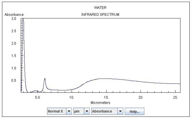
Here’s Co2
Co2 as a gas, as I understand does not emit as a BB, but with spectral emission.
Here’s water
So from space, you’d have photons from the surface, from Co2, from Water which when all mixed together I presume has a effective BB temp of 255K. If it’s measured by Pyrometer, it sums the joules from the photons and then reports it as if it’s from a BB, even if it’s all at say 193K photons, It would take a larger 15u flux (@193K) to equal a 255K BB. Now if measured by a spectrograph, you can sum the individual spectrum’s, and it would have spikes over the top of say a 180K BB which could sum to that same 255K.
Does that make sense? I’m not sure I’ve explained it very well.
Oh, NIST says the two spectrums (Co2 and Water) are not quantitatively accurate (IE the heights of the spikes are not comparable between the two).
Thanks for that.
I need to look into the individual characteristics of different GHGs including that of specific gravity which will make a difference to the balance between radiation to space and the need to support molecules higher up.
It may be that my reference to the emission height should have referred to the point of hydrostatic balance but as yet I haven’t worked out the relationship between the two.
The thing is though that if kinetic energy at the surface has to be allocated to continual collisions in order to support hydrostatic balance then that compromises the ability of the surface to emit photons.
However one cuts it a surface at 288k cannot be emitting photons at a rate commensurate with that temperature.
It has to be emitting photons at the rate commensurate with 255K and the reason is mass density at the surface taking up that additional 33K in collisional activity.
AGW theory has the surface emitting photons at 288k which cannot be right if hydrostatic balance is to be maintained.
It’s complicated, so no problem. I would suggest Feynman’s QED, and then lectures for a more scientific view of quantum absorption and emission.
Interesting that there seems to be no counter argument for my assertion that the rate of photon emission from any radiatively active material declines as one descends through atmospheric mass because collisional activity takes over from photon emissions.
The rise in temperature along the lapse rate slope is the equilibrium response to that decline in photon emissivity. The radiating material has to get warmer with depth in order for the Earth system to emit 255k to space whilst simultaneoiusly holding the mass of the atmosphere off the ground.
Being a matter of mass it follows that radiative characteristics count for nothing and in any event any thermal effect of radiative capability is negated by convective adjustments.
As far as I can see, that observation renders AGW radiative theory completely inapplicable.
Stephen Wilde May 24, 2015 at 4:23 am says:
While it is tempting to think that there is no counter argument put forth simply because you are 100% correct … it’s more than possible that there may be no counter argument because most folks do what I do, which is to only rarely read more than the first line or two of your comments. I fear that your endless streams of uncited claims and arcane explanations finally got to be too much for me.
As one example among dozens, I have no idea at all what this means:
Among the many problems with this statement is exactly what you are discussing. What is “photon emissivity” when it’s at home? I know what “emissivity” is, but this is the first time I ever heard of “photon emissivity”. You seem to equate it with the “rate of photon emission”, which I assume would be measured in something like photons per second … while emissivity is a dimensionless number that varies from zero to one. You see the difficulties faced by the scientifically-minded reader?
Nor do I have any particular interest in finding out what you mean by that convoluted statement, as doing so with you seems to lead to infinite recursion.
So, I just pass. There are too many interesting, well cited and supported comments and too little time as it is. I just wrote this to caution you that the lack of opposition could mean you are right … or it could just mean that few folks are reading your stuff any more.
Now there are a couple of ways you could take this. Let me suggest that you take it in the spirit in which it is offered, which is that of an opportunity to up your game. Read more. Learn more. Be more cautious in your claims. Explain your terms, and don’t use terms in a new unusual manner without forewarning and explanation. Dial the extent of your claims back to what you can easily defend. And please, please learn the currently accepted explanation before posting a new explanation.
As an example. Whenever you have an atmosphere that is heated from the bottom, you will get a lapse rate, with the atmosphere cooling as it rises and expands. Air is heated at the bottom, rises, expands, and must therefore cool from the expansion. This gives a “lapse rate”, a rate of decline in temperature with increasing elevation.
Now you come along and say:
The accepted explanation for the existence of the lapse rate says nothing about “photon emissivity”. Instead it says that hot air rises, and when it rises it expands, and when it expands it cools. Period. Nothing about radiative gases. Nothing about “photon emissivity”.
So if you want to be the first to claim that the existence of the lapse rate is from variations in “proton emission” whatever that might be, FIRST you have to not only understand but also refute the accepted explanation, while at the same time providing an unambiguous new explanation along with observational support for your new explanation.
And I do think that you can do that, Stephen … I do think that you can up your game to that level.
w.
Willis, I have no problem with the tone or content of your response.
I am simply pointing out that as one descends through the mass of an atmosphere the temperature of a radiative molecule has to rise in order to get 255K out to space past the barrier to energy transmission presented by conduction and convection.
If the radiative molecule is situated at the surface then for Earth it has to be at 288K to get 255k out to space.
If it is at a higher location then the temperature of the molecule has to achieve a compromise beteween its radiative capability and its specific gravity.
The basic point is that S-B does not apply and cannot apply to an interface between two grey bodies which are exchanging energy between themselves via conduction and convection.
Earth’s surface radiates 255k upward even though it is at a temperature of 288k because the other 33k is locked into the conductive/convective exchange which provides the necessary energy for the upward pressure gradient force.
May I humbly suggest that the problem is not my terms of expression but rather your unfamiliarity with concepts such as hydrostatic balance, pressure gradient force and the idea that a surface at 288k does not necessarily radiate at 288k but rather at a rate commensurate with 255k after deducting the kinetic energy locked into convective overturning in the form of potential energy?
The Dry Adiabatic Lapse Rate shows the rate at which the temperature of NON radiative molecules must be elevated at any given height in order for them to allow the surface to radiate 255K of radiation to space past the conducting and convecting mass of an atmosphere.
In connection with radiative molecules that height can be distorted by both the radiative capability and the specific gravity of the molecule because specific gravity determines how much energy needs to be expended by that molecule in lifting it against gravity. CO2 is heavier than air whereas water vapour is lighter than air so they distort the DALR differently.
It is right for you to say
“Whenever you have an atmosphere that is heated from the bottom, you will get a lapse rate, with the atmosphere cooling as it rises and expands. Air is heated at the bottom, rises, expands, and must therefore cool from the expansion. This gives a “lapse rate”, a rate of decline in temperature with increasing elevation”
but it must also follow that the reverse happens on descent.
So why does the reverse happen on descent in the absence of radiative molecules?
The only possible explanation in the absence of GHGs is that the mass of an atmosphere reduces the probability of photons being emitted as density increases and of course the lapse rate follows the density gradient.
As regards ‘upping my game’ the problem here is that I am using words and concepts to explain the way established physics works out in practice within the mass of an atmosphere. The relevant numbers already exist in the form of the Gas Laws and the hydrostatic equations so there is no need for me to rehearse them anew.
The problem is that readers have been taught an erroneous conceptual interpretation which places paramount significance on the net radiative exchanges but that is inadequate.
I need readers to up their game and look at the earlier established science in a way that was never taught to them.
A good article but one that is incomplete in the sense that there is no temperature activity attibuted to volcanoes on the vey long island arcs that occur throughout all of the major islands. Having flown the Pacific and Indian oceans as a member of the rear section I have been able to observe one interesting phenomon. The ugrading of the passenger flight maps has enable a better view of the erlationship between turbulence above 12,000m and the location of the various island arcs. The recent flight to the USA took the southern route just to the south of Pago Pago. Flying across the island arc yielded vigorous turbulence embracing the new Dreamliner. The turbulence ceased immediately once the island arc was crossed. For the next couple of hours minor turbulence occurred whenever a seamount was crossed. There were no cumuls clouds evident during the bulk of the flight. From the headwind descriptor there was very little wind direction changes in the same sector.
My point is that the map represented by Figure 4 onObserved temperatures minus the estimated temperature field, centered on the International Dateline. Gray line shows the boundary between positive and negative values also represents the boundary between turbulence and calm air. This means that the influence of volcanic island arc temperatures must be taken into consideration when prognosticating on variations in ocean temperatures.