Some updates to the Monckton et al. 'Irreducibly Simple Climate Model'

Guest essay by Joe Born

Lead author Christopher Monckton turned down my request for further information about how the Table 2 “transience fraction” values in Monckton et al., “Why Models Run Hot: Results from an Irreducibly Simple Climate Model,” were obtained from a Gerard Roe paper’s Fig. 6. Those values are implausible, so in this post we will follow Lord Monckton’s suggestion that we obtain our own $r_t$ values. We will then use the results to address some misconceptions about feedback and sensitivity to assumed stimuli.

The innovation in Monckton et al.’s model 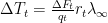$\Delta T_t=\frac{\Delta F_t}{q_t}r_t\lambda_\infty$ of the relationship between stimulus $\frac{\Delta F_t}{q_t}$ and response $\Delta T_t$ was its separating a linear model’s step response into magnitude $\lambda_\infty$ and shape $r_t$ factors. Since by definition $r_\infty=1$ , this makes the relationship between feedback $f$ and equilibrium response value $r_\infty\lambda_\infty=\lambda_\infty$ apparent because $\lambda_\infty=\lambda_0/(1-\lambda_0f)$ , where $\lambda_0$ is the no-feedback value, styled the “Planck climate-sensitivity parameter” in their paper.

“Transience fraction” is the name they gave that shape component $r_t$ : it is a normalized step response. And Roe’s Fig. 6 depicts responses to a $4\,\textrm{W/m}^2$ forcing step. So one might speculate that Monckton et al. obtained their Table 2 transience-fraction values by normalizing those Fig 6 values.

However, that graph contains only one or arguably three curves, whereas Monckton et al.’s Table 2 contains values for five. Rather than explain in response to my consequent inquiry how the authors might have accomplished this loaves-and-fishes feat, Lord Monckton simply stated: “The table was derived from a graph in Gerard Roe’s magisterial paper of 2009 on feedbacks and the climate. Far from obscuring anything, we had made everything explicit.”

Lord Monckton also issued an invitation: “If Mr Born disagrees with Dr Roe’s curve, he is of course entirely free to substitute his own.” I reluctantly accept that invitation, not because I know of any reason to reject (or accept) Dr. Roe’s curves but because the values that Monckton et al. inferred from them are implausible.

Fig. 1 depicts the step responses of which Monckton et al.’s Table 2 are normalized versions. That is, it shows the results of multiplying each row’s entries by the corresponding $\lambda_\infty=\lambda_0/(1-\lambda_0f)$ , where $1/\lambda_0=3.2\,\textrm{W/m}^2/\textrm{K}$ and $f$ is the value their table lists as $f_\infty$ . (Although Monckton et al. also use the notation “ $f_t$ ,” the $f_\infty$ values seem to be the only ones they use, so we will simply use $f$ as our feedback-coefficient symbol.)

Consider that plot’s various values for $t=25$ years. Suppose that 25 years after a $1.0\,\textrm{W/m}^2$ step in forcing we have observed a 0.24 K temperature increase. By consulting that plot, we conclude that the feedback is a modest $0.5\,\textrm{W/m}^2/\textrm{K}$ , implying an equilibrium climate sensitivity of 1.4 K. If the increase were 0.29 K instead, we would infer a rather larger $1.3\,\textrm{W/m}^2/\textrm{K}$ feedback coefficient, which implies a larger equilibrium climate sensitivity, 2.0 K. But if the temperature increase were still greater, 0.31 K, we would infer—no feedback at all. And that implies equilibrium climate sensitivity of only 1.2 K.

How’s that again? A higher current temperature increase implies a lower equilibrium climate sensitivity?

Theoretically, that result is not completely impossible; if you make different system assumptions for different feedback levels, you can get results like that. But it is far from self-evident that the Roe paper from which Monckton et al. purportedly derived their Table 2 dictates so implausible a result. So, to use Monckton et al.’s model but employ more-plausible behavior, we resort to rolling our own version of Table 2.

To that end we will model the system in the manner that Fig. 2 depicts. We use the $H_0(s)$ notation in the forward block as shorthand for its input-output relationship. Dr. Roe said his results came from a model that included diffusion, but for the sake of simplicity we’ll assume a lumped-parameter model. We arbitrarily adopt a third-order relationship between that block’s output $y$ and its input $x$ :

$\frac{d^3y}{dt^3}+q_2\frac{d^2y}{dt^2}+q_1\frac{dy}{dt}=p_2\frac{d^2x}{dt^2}+p_1\frac{dx}{dt}+p_0x$ .

For reasons that will become apparent in due course we adopt the following coefficient values: $q_2=1.7\times 10^{-9}\textrm{sec}^{-1}$ , $q_1=3.2\times 10^{-19}\textrm{sec}^{-2}$ , $p_2=9.8\times 10^{-10}\,\frac{\textrm{K/sec}}{\textrm{W/m}^2}$ , $p_1=4.2\times 10^{-19}\,\frac{\textrm{K/sec}^2}{\textrm{W/m}^2}$ , and $p_0=1.8\times 10^{-29}\,\frac{\textrm{K/sec}^3}{\textrm{W/m}^2}$ .

Fig. 3 depicts the response that such a system exhibits when its input $x$ is a unit step: it asymptotically approaches a linear increase without bound. This is what we would expect of a system that steadily receives heat but sheds no heat in response.

To obtain the step responses for the various levels of feedback in Monckton et al.’s Table 2, we add feedback, as our Fig. 2’s feedback block indicates. This is a simple matter of replacing $y$ with $\Delta T$ and replacing $x$ with $\Delta F + f_{tot}\Delta T$ for respective values of total-feedback coefficient $f_{tot}\equiv f-1/\lambda_0$ :

$\frac{d^3}{dt^3}\Delta T+q_2\frac{d^2}{dt^2}\Delta T+q_1\frac{d}{dt}\Delta T=p_2\frac{d^2}{dt^2}(\Delta F + f_{tot}\Delta T)+p_1\frac{d}{dt}(\Delta F + f_{tot}\Delta T)+p_0(\Delta F + f_{tot}\Delta T)$ .

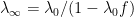
Fig. 4 depicts the solutions to that equation for a unit step in forcing and shows that they approximate all Monckton et al. Table 2 values except the implausible $f=0$ entries. This is not entirely coincidental, since the open-loop equation’s coefficients were so chosen as to make the normalized solution to the corresponding closed-loop equation approximate the entries in one of Table 2’s rows.

The $r_t$ values that correspond to the Fig. 4 solutions take the form

$r_t = 1 - A_1 e^{-t/\tau_1} - A_2 e^{-t/\tau_2} - A_3 e^{-t/\tau_3},\qquad \sum A_i=1.$

For the feedback values in Monckton et al.’s Table 2, the coefficients are as follows, with the $\tau_i$ ’s given in years:

Recall that the total-feedback values $f_{tot}$ we used to obtain those $r_t$ values were sums of the climate-science-style feedback $f$ values and the negative reciprocal $-1/\lambda_0$ of what Monckton et al. call the “Planck climate-sensitivity parameter.” Lord Monckton has <a href=http://wattsupwiththat.com/2015/03/16/where-the-complex-climate-models-go-wrong/#comment-1887123>objected</a> to my having done so: “The misinterpretation – commonplace, but wrong – is in his assumption that the Planck parameter is a feedback just like all the others. No. In fact, it plays a special role in the determination of climate sensitivity, is not summed with the true feedbacks but is, uniquely, instead multiplied by their sum, is separately multiplied by the initial forcing to determine zero-feedback warming, again unlike any of the true feedbacks. . . .”

That objection is largely conceptual rather than substantive. Response curves exactly the same as Fig. 4’s would have resulted if the calculations had been based on the block diagram of Fig. 5 rather than that of Fig. 2. Note that, as Lord Monckton prefers, the feedback-block legend in Fig. 5 is simply $f$ rather than $f-1/\lambda_0$ . Note also that the legend on Fig. 5’s forward block is $H_\lambda(s)$ instead of $H_0(s)$ : Figs. 2 and 5 have different relationships between forward-block output and input. Instead of the open-loop equation given above for $H_0(s)$ , the equation for $H_\lambda(s)$ is the one that results from the above closed-loop equation when $f$ is set to zero: its step response is the solid black curve in Fig. 4.

Now, that response’s $t=\infty$ value is $\lambda_0$ , so the loop gain is indeed $\lambda_0f$ : in a sense, as Lord Monckton says, the “Planck parameter . . . is not summed with the true feedbacks but is . . . instead multiplied by their sum.” But that characterization results merely from the way in which we defined the system and from the level of abstraction we used. The Fig. 5 diagram is merely a higher-level version of Fig. 6, which shows that Fig. 5’s forward block is itself a feedback system. And by the distributive property Fig. 6 is equivalent to Fig. 2, from which we derived our transience-fraction values. So, as far as Monckton et al.’s linearized model goes, little depends on whether the “Planck parameter” is thought of as a feedback quantity: Lord Monckton has objected to form, not substance.

It bears emphasis at this point that Lord Monckton was correct in saying that “in all runs of our model that concerned equilibrium sensitivity (and most of them did) [the transience fraction $r_t$ ] is simply unity”: the relationship between feedback and equilibrium sensitivity does not depend on Monckton et al.’s having gotten the transience fraction right. Moreover, Monckton et al. were modest in their claims for the model, referring to the “rough and ready fashion” in which it represented forcings and feedbacks and pointing out that the model’s use is “narrowly focused on determining the transient and equilibrium responses of global temperature to specified radiative forcings and feedbacks in a simplified fashion.”

The model is advisedly simplified, intended to be simple enough that the authors could commend its use to “those who have no access to or familiarity with the general-circulation models,” just “a working knowledge of elementary mathematics and physics.” And Lord Monckton quite understandably turned down requests for computer code on the basis that users could readily implement the model on a pocket calculator and thereby “be determining climate sensitivity more reliably than the [IPCC] in minutes.”

But the latter feature is the result of the fact that their model $\Delta T_t=\frac{\Delta F_t}{q_t}r_t\lambda_\infty$ simply multiplies the time- $t$ value $\frac{\Delta F_t}{q_t}$ of the stimulus by the time- $t$ value $r_t\lambda_\infty$ of the step response rather than, as would be more conventional, convolving entire time sequences. And, at least as implemented, that feature appears to have resulted from failure to heed Mark Twain’s admonition that we “be careful to get out of an experience only the wisdom that is in it and stop there.”

In response to my observation that, as he put it, “we relied on a model generated by a step-function representing the effects of a sudden pulse in CO2 concentration rather than one in which concentration increases by little and little,” Lord Monckton admitted that they had indeed relied on a step stimulus. But he justified that approach with wisdom he had gotten out of a related experience:

“I had first come across the problem of stimuli occurring not instantaneously but over a term of years when studying the epidemiology of HIV transmission. My then model, adopted by some hospitals in the national health service, overcame the problem by the use of matrix addition, but sensitivity tests showed that assuming a single stimulus all at once produced very little difference compared with the time-smeared stimulus, merely displacing the response by a few years. Similar considerations apply to the climate.”

Even for “determining the transient and equilibrium responses of global temperature,” that experience may have had rather less wisdom than Lord Monckton supposed.

Fig. 7 illustrates transient climate response, i.e., the temperature increase that will have resulted at the time when CO2 concentration has doubled after increasing by 1% per year. The legend in the upper left gives the equilibrium climate sensitivities that Monckton et al.’s Table 2 feedback values imply: it gives the changes in temperature that would ultimately result if that doubled concentration remained in perpetuity. For the corresponding systems, whose step responses Fig. 4 depicts, Fig. 7’s solid curves represent the responses to an instantaneous CO2-concentration doubling, and its dashed curves represent corresponding responses to doubling over about 70 years ( $1.01^{70}\approx 2$ ).

If after the 70 years in which CO2 concentration has doubled we observe the 1.7 K temperature change marked by an “x” on that the plot, then the equilibrium climate sensitivity inferred by the Monckton et al. approach, i.e., from multiplying the current stimulus value by the current step-response value, would be the 3.4 K associated with the solid curve closest to the marked value at 70 years. But the equilibrium climate sensitivity inferred from the more-conventional approach of convolving the stimulus’s derivative with respective step responses would be more like the 12.4 K associated with the closest dashed curve.

There are those who would consider such a difference significant.

Again, this does not mean that the Monckton et al. model is completely unworkable. In particular, I know of no specific problem with the results it gives for the $t=\infty$ , i.e., unity-transience-fraction, case. Moreover, although we have seen that the Monckton et al. approach has significant problems in principle, it would be hard to tell without a more-detailed account of underlying data and assumptions how significantly those problems may have affected the numerical results at which Monckton et al. arrived in practice.

Also, although we have seen that the difference between Monckton et al.’s simple multiplication and the more-accurate, conventional convolution approach can be significant, a simple-multiplication approach may still be justified if the expected forcing trajectories are obliging enough. If the trajectories that the forcings $\frac{\Delta F_t}{q_t}$ follow are expected to be roughly linear, for example, one could adopt $r_t$ values based on a ramp response rather than the step response from which Monckton et al. obtained theirs.

But it is not clear that those conditions apply. In short, Monckton et al.’s model has limitations of which “the user manual for the simple model, bringing it within the reach of all who have a working knowledge of elementary mathematics and physics” omits warnings the reader could have profited from. At the very least, users should exercise caution when they use the model’s $r_t$ values.

0 0 votes

Article Rating

160 Comments

Inline Feedbacks

View all comments

Rob F.

April 1, 2015 8:43 am

Just give me the temperature data, the whole temperature data and nothing but the temperature data. The RAW data. From good locations. No “transformation”, “normalization”, “adjusted” or otherwise manipulated. And, for the powers that be, base political decisions on the data, the whole data and nothing but the data.
The data will find you out.
The data will set you free.

Steven Mosher

Reply to Rob F.

April 1, 2015 9:56 am

Ghcn daily.
It’s been there for years.

Salvatore Del Prete

April 1, 2015 8:48 am

http://www.ipcc.ch/publications_and_data/ar4/wg1/en/ch10s10-3-5-6.html
Dodgy another blunder AGW has made.

sabretruthtiger

April 1, 2015 9:06 am

Today is April 1st. When Anthony reposts this on another day I’ll believe it 🙂

Bill McCarter

April 1, 2015 9:30 am

Ceteris paribus, We get lost looking at just one tree in a very big forest, and a very small tree at that. Looking to co2 to being the operator of climate is equivilent to looking to tire pressure as the control system of my car. Temperature is a very lousy proxy for climate, and is used as the “jingling of keys” to distract our attention.

Kevin Kilty

April 1, 2015 9:32 am

Joe Born April 1, 2015 at 4:55 am
What matters is that scientific papers be clear and rigorous…
The impression one gets is of a large body of literature largely untouched by human minds….
Perhaps an occasional critical review will tend to improve the situation.

Thank you for all this effort. I teach a system dynamics course, and so I enjoy seeing some of the concepts of that course applied to an unusual problem.
You have three great quotes in one sort post, here. One thinks that critical reviews would solve many problems — from wasted scientific effort to government malfeasance, but I have found that most people have difficulty understanding a critical review and believers just barge past them anyway. Your second comment about scientific results untouched by human minds is very amusing. Even when some particular topic is well analyzed, there seems always more to investigate. Climate science seems particularly rich in this way.

Joe Born

Reply to Kevin Kilty

April 1, 2015 6:05 pm

Thanks for the kind words.
I take your point that the benefits of critical review tend to be modest. I just like to hope they aren’t non-existent.

Steven Mosher

April 1, 2015 9:54 am

Joe
Nice work.
It’s a shame that William Briggs and Monkton have resorted to the tricks of the team by refusing to clearly explain and document all their steps. Jones used the same trick to thwart Mcintyre.
Please try again and this time send an open letter to all the authors requesting an explanation.

Patrick

Reply to Steven Mosher

April 1, 2015 10:21 am

So only know you see an “issue”?

mothcatcher

Reply to Steven Mosher

April 1, 2015 1:07 pm

Agreed, so they should. Even if the dispute is not fundamental to the main argument. Lord M doesn’t usually duck a challenge, and this is a direct and specific one. However, some of the comments here (esp. Gary Pearse, 6.24 a.m) allude to a broader perspective which gets a lot of points from me. Theoretical math has its limits in this debate.

Monckton of Brenchley

Reply to Steven Mosher

April 3, 2015 3:47 am

Mr Mosher would perhaps benefit from reading our paper before assuming that what Mr Born asserts we have “refused” to explain is not therein explained.

Steven Mosher

Reply to Monckton of Brenchley

April 3, 2015 7:08 pm

post your code

Steven Mosher

April 1, 2015 12:28 pm

“The model is advisedly simplified, intended to be simple enough that the authors could commend its use to “those who have no access to or familiarity with the general-circulation models,” just “a working knowledge of elementary mathematics and physics.” And Lord Monckton quite understandably turned down requests for computer code on the basis that users could readily implement the model on a pocket calculator and thereby “be determining climate sensitivity more reliably than the [IPCC] in minutes.”
This repeats Santer’s argument with McIntryre.
The argument is this.
A. The calculation is so simple that I DONT have to provide it.
So, Monkton has stolen Santer’s trick.
There are two tricks that people like Santer, Jones, and Monkton use.
Trick A: There is IP.. that is the trick is ours to keep
Trick B: It’s trivial.
But if its trivial then there is NO REASON NOT TO SHARE IT.
Here is Santer.. Looks like Monkton went to Santer school
“Dear Mr. McIntyre,
I gather that your intent is to “audit” the findings of our recently-published paper in the International Journal of Climatology (IJoC). You are of course free to do so. I note that both the gridded model and observational datasets used in our IJoC paper are freely available to researchers. You should have no problem in accessing exactly the same model and observational datasets that we employed. You will need to do a little work in order to calculate synthetic Microwave Sounding Unit (MSU) temperatures from climate model atmospheric temperature information. This should not pose any difficulties for you. Algorithms for calculating synthetic MSU temperatures have been published by ourselves and others in the peer-reviewed literature. You will also need to calculate spatially-averaged temperature changes from the gridded model and observational data. Again, that should not be too taxing.
In summary, you have access to all the raw information that you require in order to determine whether the conclusions reached in our IJoC paper are sound or unsound. I see no reason why I should do your work for you, and provide you with derived quantities (zonal means, synthetic MSU temperatures, etc.) which you can easily compute yourself.
I am copying this email to all co-authors of the 2008 Santer et al. IJoC paper, as well as to Professor Glenn McGregor at IJoC.
I gather that you have appointed yourself as an independent arbiter of the appropriate use of statistical tools in climate research. Rather that “auditing” our paper, you should be directing your attention to the 2007 IJoC paper published by David Douglass et al., which contains an egregious statistical error.
Please do not communicate with me in the future.
Ben Santer

Tom Trevor

Reply to Steven Mosher

April 2, 2015 8:03 am

Wow, you’ve gone off the deep end even for you, Mosher. Ben Santer wrote those things, not Monkton. If want to criticize Monkton why not try quoting him?

Steven Mosher

Reply to Tom Trevor

April 3, 2015 7:11 pm

The point is that Monkton is USING Santer’s argument. Santers argument was that he didnt have to supply his code because it was trivial. Monkton is plagarising his argument

Poptech

Reply to Tom Trevor

April 7, 2015 11:42 am

Mosher does this nonsense to try and bully skeptics with his absurd comparisons.

ChipMonk

Reply to Steven Mosher

April 3, 2015 10:22 pm

Mr. Mosher, speaking of “posting” content, can you please provide a full list of 1st-person (yourself with colleagues) research and finding you have created and/or contributed to?
Meanwhile you might find the following interesting: https://pielkeclimatesci.wordpress.com/?s=land+use
Be sure to follow the “older posts” links at the bottom of each page.
Your arguments here might be more helpful without YELLING at people, unless you want to continue using:
Trick C: yell at people until they agree with you.

ChipMonk

Reply to ChipMonk

April 3, 2015 10:43 pm

Mr. Mosher, I was trying to better understand your perspective but I don’t know if this is you:
http://www.populartechnology.net/2014/06/who-is-steven-mosher.html
Please clarify, Thanks.

Poptech

Reply to ChipMonk

April 7, 2015 11:40 am

Yes that is Mosher the non-scientist.

BobG

April 1, 2015 2:24 pm

Joe Born indicated he is a retired lawyer. While I don’t have anything against lawyers, I have found the few I know are “slippery”. They rarely lie outright but some of them are very fond of leading others to come to incorrect conclusions.
It could happen a few ways. Such as making “a request” that comes in the form of a comment to a blog post. You will notice that Joe Born included a link to the entire long thread – but not to a single request. There were many comments on the thread. No one who has a life outside of blogging could have replied to all of the comments and questions before the admin closed comments after a time to that thread.
If Joe Born didn’t email Monckton or contact him outside of the thread, then his comment is without reasonable basis and is deliberately misleading. If he did contact him, he should provide the entire exchange so that others can judge if the request is reasonable, if he waited a reasonable time for an answer and how forthcoming Monckton was.

Joe Born

Reply to BobG

April 1, 2015 5:06 pm

The third sentence of my earlier post said that “the Monckton et al. paper obscures the various factors that should go into selecting [ $r_t$ ],” and the bulk of the post thereafter was directed to what was not clear about that “parameter.” Included was the statement that “In a manner that their paper does not make entirely clear, they inferred the Table 2 relationship from a paper by Gerard Roe.”
I confess my failure to consider the possibility that as a way of eliciting a more-detailed explanation of how Monckton et al. arrived at their $r_t$ more thoroughly this approach would be too subtle. And perhaps I was too hasty in inferring from Lord Monckton’s following statement that it wasn’t: “The table was derived from a graph in Gerard Roe’s magisterial paper of 2009 on feedbacks and the climate. Far from obscuring anything, we had made everything explicit.”
So let me make amends. Here goes:
How did you guys get $r_t$ from the Roe paper?

Phil.

Reply to Joe Born

April 2, 2015 9:35 am

I guess it’s part of the non-existent appendix which Monckton promised to provide?
Monckton of Brenchley January 21, 2015 at 12:39 pm
Try the supplementary material. If the appendix was inadvertently deleted, I’ll send a copy. However, it was only in the appendix, where the system-gain equation for non-linear feedbacks was given, that it was necessary to acknowledge Gerard Roe’s derivation of it: the non-linear form of the equation does not appear elsewhere in the paper. We did try to persuade the editors to send us a copy of the supplementary material as prepared for publication, but we did not receive it.

BobG

Reply to Joe Born

April 2, 2015 9:50 am

If I wanted to get a response from Monckton on your question, I would first of all make sure it is somewhat formal before I indicate that he refused to provide the data. That is, send the authors – Monckton et. all an email. The request then could be very simple, “I’m writing a response to your paper. I can’t figure out how you guys get rt from the Roe paper. Could you show how this was done so that I can reproduce the result?”
If you don’t get a response from a blog comment, it means little. It could be that he allocates X time to blogging and ran out of time or skims the comments and didn’t see your comment or sees a 100 comments and replies to a few of them given his time constraints. But I don’t imagine for a second you didn’t already realize all of the above.
Writing, “Lead author Christopher Monckton turned down my request for further information about how the Table 2 “transience fraction” values in Monckton et al.” at the start of your blog gave me the impression that you had communicated outside of the blog (which would be what would be expected) with Monckton et al and they had refused to provide more details. I can’t imagine personally writing what you did otherwise – because it is a harmful and untrue accusation that should not be made lightly. Then I remembered you were a retired lawyer and then your comment began to make sense in that the motive is probably not about figuring anything out or about science at all.

Phil.

Reply to Joe Born

April 2, 2015 10:43 am

In the responses to his first post concerning his paper monckton usually replied to questions by saying “read the paper”. The following is typical:
Monckton of Brenchley January 21, 2015 at 8:10 am
“Phil.” should read the paper before criticizing it. The derivation of the system-gain relation as it applies to non-linear temperature feedbacks is acknowledged in the appendix in which the derivation appears. My emphasis added.
When challenged about where that appendix could be found monckton responded:
Try the supplementary material. If the appendix was inadvertently deleted, I’ll send a copy. However, it was only in the appendix, where the system-gain equation for non-linear feedbacks was given, that it was necessary to acknowledge Gerard Roe’s derivation of it: the non-linear form of the equation does not appear elsewhere in the paper. We did try to persuade the editors to send us a copy of the supplementary material as prepared for publication, but we did not receive it.
When told that there was no accessible appendix/supplementary information monckton went quiet and we didn’t get the promised copy!
Expecting to get a straight answer from monckton is a forlorn hope I’m afraid.

BobG

Reply to Joe Born

April 2, 2015 12:23 pm

Phil, did you email Monckton or co-authors about not getting the appendix?

Joe Born

Reply to Joe Born

April 2, 2015 6:06 pm

Since the phrases “inquiry” and “turned down” were hyperlinked to the inquiry and the turning down, one is entitled to question either the intellect or the sincerity of someone who professes to have thought the inquiry occurred in a communication outside the blog. In either case little is to be gained by further communication with such a personality.
Others may be interested in knowing, however, that I have in the past actually taken BobG’s proposed approach. A prolific contributor to this site had posted a proof widely hailed as being simple, elegant, and literally irrefutable, whereas I had recognized it as a farrago of latent ambiguities and unfounded assumptions. I went to the trouble of explaining that in detail and e-mailed the explanation to him. No response other than acknowledgment that he had received my missive.
I see little value in repeating such an exercise.

Phil.

Reply to Joe Born

April 2, 2015 6:53 pm

BobG April 2, 2015 at 12:23 pm
Phil, did you email Monckton or co-authors about not getting the appendix?
No he declined to answer and ran away. He knows there is no appendix.

Monckton of Brenchley

Reply to Joe Born

April 3, 2015 3:52 am

Bob G, not Mr Born, is correct. Mr Born did not explicitly ask how we determined our approximate values for the transience frepactiin until so late in the day – and in a startlingly discourteous fashion – that I could not have commented even if I had wanted to. Comments had for some reason been closed on that thread.

Monckton of Brenchley

Reply to Joe Born

April 3, 2015 3:53 am

In response to Phil., if he emails me I will send him the appendix.

Joe Born

Reply to Joe Born

April 3, 2015 8:49 am

“Mr. Born did not explicitly ask how we determined our approximate values for the transience [fraction] until so late in the day – and in a startlingly discourteous fashion – that I could not have commented even if I had wanted to.”
The title of my previous post was, “Reflections on Monckton et al.’s ‘Transience Fraction.’” I said in that post that their paper “obscures the various factors that should go into selecting that parameter.” I further said that Monckton et al. had inferred their Table 2 $r_t$ values from the Roe paper “[in] a manner that their paper does not make entirely clear.”
It taxes even my credulity to believe this left unobvious my belief that Monckton et al.’s determination of the transience fraction $r_t$ wasn’t clear enough. Yet Lord Monckton’s subsequent post did nothing to clarify it.
So I tried the 2×4-between-the-eyes approach: my first comment in the ensuing thread included code that would enable him not only to create this head post’s Fig. 1, in which I illustrated the implausibility of Monckton et al.’s Table 2 values, but also to see the data behind it. Since Lord Monckton was still commenting in that thread two days later, it strikes me as passing strange that he considers that “late in the day.”
In any event, he provided no relevant information. Hence the head post.
I truly had not intended to tax Lord Monckton’s powers of inference so sorely. And I’m grieved that he finds it discourteous that I am thus pressing him for further information. Still, he can avoid having his sensibilities further offended by simply providing the information that the original paper should have contained.

Phil.

Reply to Joe Born

April 3, 2015 9:28 am

Monckton of Brenchley April 3, 2015 at 3:53 am
In response to Phil., if he emails me I will send him the appendix.
Please just post it here so that everyone can have access to it.

Salvatore Del Prete

April 1, 2015 2:47 pm

http://media.al.com/news_huntsville_impact/photo/christy-atmosphere-temps-4fe93b1801f915d6.jpg
What the models predicted which is no where to be found.

Brian H

Reply to Salvatore Del Prete

April 2, 2015 3:12 am

In most radiosonde charts I see a slight cool spot there.
BTW, I gather the HotSpot is supposed to be the signature of any Warming “forcing”, not just AG.

Monckton of Brenchley

Reply to Brian H

April 3, 2015 3:59 am

I had the honor of giving the hot spot its name. Actually, Santer 2003 wrongly assumed the hot spot was a feature unique to anthropogenic warming. Theory would lead us to expect a hot spot whatever the cause of the warming. It’s absence indicates either that there is no warming or that either the surface or the mid-troposphere temperatures are wrongly measured. It is more likely that surface than mid-trop temperatures in the tropics are inadequately measured.

Sturgis Hooper

Reply to Brian H

April 3, 2015 9:31 am

I gave the wet spot its name.
Just kidding…

Dan Pangburn

April 1, 2015 4:42 pm

A simpler proof that CO2 has no significant effect on climate and identification of what actually does cause climate change (95% correlation since before 1900) are at http://agwunveiled.blogspot.com

jim heath

April 1, 2015 5:46 pm

I bought an air conditioner and my climate is perfect

Ed Moran

April 2, 2015 2:03 am

Although the math needed to follow the detail is way beyond me I’ve been encouraged that “Monkton v Born” has enabled a real debate. Now try to imagine this over at Sceptical Science.
Thanks Mr Watts.

Salvatore Del Prete

April 2, 2015 8:30 am

AGW theory has predicted thus far every single basic atmospheric process to be wrong.
In addition past historical climatic data shows the climate change that has taken place over the past 150 years is nothing special and has been exceeded many times over in similar periods of time, in the historical climatic record. I have yet to see data showing otherwise.
Data has also shown CO2 has always been a lagging indicator not a leading indicator. It does not lead the temperature change. If it does I have yet to see data confirming this.
SOME ATMOSPHERIC PROCESSES AND OTHER MAJOR WRONG CALLS.
GREATER ZONAL ATMOSPHERIC CIRCULATION -WRONG
TROPICAL HOT SPOT – WRONG
EL NINO MORE OF -WRONG
GLOBAL TEMPERATURE TREND TO RISE- WRONG
LESSENING OF OLR EARTH VIA SPACE -WRONG
LESS ANTARCTIC SEA ICE-WRONG
GREATER /MORE DROUGHTS -WRONG
MORE HURRICANES/SEVERE WX- WRONG
STRATOSPHERIC COOLING- ?? because lack of major volcanic activity and less ozone due to low solar activity can account for this..
AEROSOL IMPACT- WRONG- May be less then a cooling agent then expected, meaning CO2 is less then a warming agent then expected.
These are the major ones but there are more. Yet AGW theory lives on.

Bernie Hutchins

April 2, 2015 9:49 am

Joe –
Many thanks for the idea from your earlier posts of putting in the capacitor. It adds insight to SEE SOMETHING HAPPENING rather than to see that something HAS HAPPENED.
Three days ago I posted a discussion of your circuit as a nice feedback example:
http://electronotes.netfirms.com/ENWN25.pdf
It is an extension of the figures I posted in a previous thread. In addition, last evening I decided to actually just do it by inverse Laplace transforms. MUCH simpler than I was supposing, and it comes out to two terms – one LP and one HP.
http://electronotes.netfirms.com/JB2.jpg
The LT results are identical to the previous simulations, and offer more insight. Rather than just the final endpoint, we watch it get there.

Joe Born

April 2, 2015 6:03 pm

An interesting aspect of your discussion was the frequency response for a greater-than-unity loop gain: it’s finite. For a purely sinusoidal stimulus, the output remains within limits (in theory). For a sinusoid that doesn’t start until t = 0, though, the response blows up unless (in theory, of course) the phase at t = 0 is just right: in the output a finite-amplitude sinusoid is superimposed on an exponential whose polarity and magnitude depend on the sinusoid’s t = 0 phase.
In practice, of course, the output always blows up, and polarity will be unpredictable because it’s highly sensitive to initial conditions.
By the way, you parsed the amplifier’s step response in a way I hadn’t considered. For myself I first worked it out in Laplace transforms, of course, but I looked at the impulse response as the sum of a Dirac delta of amplitude A (going straight through the amplifier) and a low-pass of amplitude A^2 f / (1 – Af) (following the feedback). Equivalent, of course, but it’s always interesting to look at something from a different angle.

Kevin Kilty

April 3, 2015 9:43 am

Joe Born,
I have had a few days to ponder your article, and I have a couple of points that you might respond to if you care to and have time. First, when I first read the Monckton et al paper, my impression was that they intended this to be a simple procedure of doing forward calculations–i.e. the user could make assumptions about r and q and f, and see what the results would be of Delta T in time. I should perhaps return to their paper and read it again, but that was my point of reference for evaluating their work. Moreover, I also assumed that by using the subscript “t” for r and q they were implying that these might be functions of time.
It makes more sense, perhaps, to see q as a function of temperature, but that renders the problem non-linear again which runs counter to their purpose. Your point regarding convolution of source function and impulse response function is well taken and absolutely correct, but amateurs are not going to program a convolution on a hand calculator. However, a convolution integral results in a function of time; and r, as a general function of time bound by the value 1 as t approaches infinity, is capable of absorbing this. The flaw in Monckton et al is to not discuss this, or to provide guidance on how to go about formulating r so that it approximates use of a convolution integral well.
There was discussion around the internet soon after their paper appeared, with severe criticism about them having made an instantaneous model where temperature changes everywhere instantly–an invalid criticism. I could not see how such criticism arose, but your discussion has helped me understand this better. The parameter r is not intuitive. Point well taken.
Second, in your Figure 4 you show an inverse problem–that of finding the value of some parameter of climatological interest, from temperature observations at particular times. Once again I need to go back and re-read Monckton et al with new eyes, but my understanding of their purpose was that they intend forward calculations. Algorithms that are successful in a forward sense are sometimes just awful in the inverse sense. For instance, my students make temperature measurements of a cooling fin from its root to tip. Some of these students then find a spline function that allows them to calculate temperature at any point on the fin–a forward calculation for which the spline function is a perfectly good model. However, my purpose is for them to find the film coefficient from these measurements–a inverse calculation; and, the spline is worthless for this purpose because none of its parameters relates to film coefficient clearly.
Your Figure 4 gives readers the impression of terrible forward calculation ability, when in fact it shows lousy inverse problem capability if misused. Once again it is the non-intuitive r value, but inverse problems need to be specified and formed quite carefully before rendering a judgement. I found Monckton et al’s paper to be very thought provoking; and I bet it provoked lots of thought in various quarters. Your contribution has clarified some important points.

Joe Born

Reply to Kevin Kilty

April 3, 2015 2:39 pm

Kevin Kilty: “[W]hen I first read the Monckton et al paper, my impression was that they intended this to be a simple procedure of doing forward calculations–i.e. the user could make assumptions about r and q and f, and see what the results would be of Delta T in time.”
That’s my impression, too.
Kevin Kilty: “Moreover, I also assumed that by using the subscript “t” for r and q they were implying that these might be functions of time.”
That’s what I think, too.
Kevin Kilty: “It makes more sense, perhaps, to see q as a function of temperature, but that renders the problem non-linear again which runs counter to their purpose.”
I’m not sure I see why that would make more sense, but, in any case, that possibility hadn’t occurred to me.
Kevin Kilty: “[A]mateurs are not going to program a convolution on a hand calculator. ”
I know that this amateur wouldn’t be inclined to.
Kevin Kilty: “However, a convolution integral results in a function of time; and r, as a general function of time bound by the value 1 as t approaches infinity, is capable of absorbing this.”
True, but only if you know the shape of the stimulus curve in advance.
Kevin Kilty: “The flaw in Monckton et al is to not discuss this, or to provide guidance on how to go about formulating r so that it approximates use of a convolution integral well.”
That’s exactly my point. I attempted in my first post to elicit more details about that function. All I got was a debate; he said they’d already told us everything. My second post’s purpose was to give examples of how that wasn’t necessarily so.
As to the last two paragraphs of your comment, I’m not sure I follow the “forward” and “reverse” nomenclature, but I guess that’s what I get for mucking about in your area. Anyway, in Fig. 4 I was just trying to come up with a more-plausible relationship among the various-feedback systems’ step responses. I don’t follow your abstraction to “finding the value of some parameter of climatological interest.”

BobG

Reply to Joe Born

April 3, 2015 10:36 pm

Being an engineer who has from time to time used feedback equations in my work, and am therefore familiar with the concepts and equations, I found no real issues with Monkton et al.
The intended purpose was give as: “. It is intended to enable even non-specialists to study why the models are running hot and to obtain reasonable estimates of future anthropogenic temperature change.
The model is calibrated against the climate-sensitivity interval projected by the CMIP3 suite of models and against global warming since 1850. Its utility is demonstrated by its application to the principal outputs of the CMIP5 models and to other questions related to climate sensitivity.”
The model is a model used for investigation purposes. I put into a spreadsheet Monckton’s model as it was the simplest and fastest way for me to implement such that I could change the values and create graphs. It took a few minutes to put in the spreadsheet and a while longer to comprehend the variables. It worked as Monckton et al claimed.
Looking at Joe Born’s comments about his quibbles with rt and the Monckton et al model appear as he put it, “largely conceptual rather than substantive.” This is confirmed later when Joe Born wrote, “It bears emphasis at this point that Lord Monckton was correct in saying that “in all runs of our model that concerned equilibrium sensitivity (and most of them did) [the transience fraction r_t] is simply unity”: the relationship between feedback and equilibrium sensitivity does not depend on Monckton et al.’s having gotten the transience fraction right. ”
About rt, “rt is the transience fraction,which is the fraction of equilibrium sensitivity expected to be attained over t years; … In Eq. (1), the delay in the action of feedbacks and hence in surface temperature
response to a given forcing is accounted for by the transience fraction rt.” … “For instance, it has been suggested in recent years that the long and unpredicted hiatus in global warming may be caused by uptake of heat in the benthic strata of the global ocean (for a fuller discussion of the cause of the hiatus, see the supplementary matter). The construction of an appropriate response curve via variations over time in the value of the transience fraction rt allows delays of this kind in the emergence of global warming to be modeled at the user’s will.”
The more times I read Joe Born’s issues with Monckton et al’s use of rt, the stranger it seems. That is because rt behaves from the modeler’s point of view the way I would expect from the discussion. In other words, used in the equation in the described way, it works as described. With respect to whether the transient fraction values that Monckton et al derived were implausible or not that came from Gerard Roe paper’s figure 6, this is not a substantial point. It is rather a small quibble given the purpose of the model and the use of rt in the equation and the fact that as Joe Born noted, the feedback and equillibrium sensitivity does not depend on this fraction being right. A quibble it seems to me that Job Born built up to a huge mountain and turned into what seems to be a mean spirited attack.

Monckton of Brenchley

Reply to Kevin Kilty

April 5, 2015 4:29 am

In response to Mr Kilty, there is in fact quite a bit of discussion in our paper (and more in the appendix) about the representation of the feedback-driven non-linearities in climate response in our model. The transience fraction is the simplest way to handle this. Remarkably, given that feedbacks account for two-thirds of warming in the IPCC’s understanding, time-series graphs of the non-linear evolution of temperature change in the IPCC’s documents are crude and not well explained or justified. We therefore used Roe’s three evolutionary curves as the basis for our table of approximate values.
As to the convolution-vs.-pulse point, we cited in full Roe’s caption making it plain that his curve is based – like many of the curves the general-circulation models and the IPCC produce – on an initial pulse of forcing. We also demonstrate, with worked examples, that the IPCC’s response curve is linear for the first 100 years or so, by which time about half of equilibrium sensitivity will have been attained. And we thrice explain that our values for the transience fraction are approximate. We explicitly state that the user of the model is free to adopt his own values, and almost an entire pages is devoted to discussing these values. Mr Born, in saying we have refused to explain how our values for the transience fraction are obtained, is not only discourteous but erroneous.
As to the question whether convolution-vs.-pulse makes any difference, it is at last agreed even by Mr Born that at equilibrium the value of the transience fraction is by definition unity, convolution or no convolution. And the main thrust of our paper was of course directed towards equilibrium sensitivity.
However, we did also provide worked examples for each of the six RCP concentration pathways to 2100. It will be seen that, in line with our substantial discussion in the paper of the IPCC’s implicit centennial values, we used values 0.5-0.7 for our transience fractions. Now, if one does not determine the convolution integral – which our simple model of course did not do, for we wanted to keep it simple – the consequence is that climate sensitivity will be somewhat overstated in the model. If, therefore, the model is run and shows a significantly lower climate sensitivity than the general-circulation models, then of course a model run on the basis of a convolution interval – which is, of course, time-dependent, as Mr Kilty rightly points out – will show even less climate sensitivity.
Furthermore, the values of individual feedbacks cannot be determined to sufficient precision either empirically or theoretically, nor can we even distinguish the relative magnitudes of forcings and feedbacks. The value of using a single, simple parameter to encompass all of the feedback-driven non-linearities in the climate system response is, of course, that users of the model can readily determine the starting-point (feedback sum zero; system gain 1; transience fraction transient/equilibrium sensitivity); can adopt or not adopt the IPCC’s estimate that half of equilibrium warming occurs after 100 years; and can use our own approximations of the transience fraction as a rough guide. In a simple model, one cannot really do a lot better than that.
The proof of the pudding, of course, will be in the eating. Our model predicts 0.9 K manmade warming by 2100. At present, during a negative PDO phase, the underlying warming rate, which is the rate at which the oceans are warming (if the ARGO measurements were to sufficient precision) is about 0.25 K/century. Of course, much of the CO2 we shall put into the air from now to 2100 is not there yet, and there will be a positive PDO phase from about 2025-2060, so our rough and ready model does seem to be generating predictions that are not by any means unreasonable.
Of course, our best estimate is that negative feedbacks prevail in the climate: otherwise the remarkable thermostasis of the past 810,000 years is rather difficult to explain. In those circumstances, the pulse-vs.-convolution question becomes near-entirely academic. To raise it at all is to require a degree of precision that the resolution of the data and the detail of the theory are in any event unable to support. There are, no doubt, rigorous methods of determining how many angels dance on the head of the average pin, but in the long run your guess is as good as mine. The transience fraction provides a simple and actually quite powerful method of allowing the user of the model to make a coherent guess.

Monckton of Brenchley

April 3, 2015 7:31 pm

Mr Born’s quarrel is with the IPCC, not with me. They have provided no feedback response curves over time, except postage-stamp-sized climate-sensitivity curves – with no data to support them – in AR4 at Fig. 10.26 on p. 803. So we took Roe’s curve and did not worry about convolutions, because the uncertainties in the determination of feedbacks are so large that they swamp such considerations. One can of course, as Mr Born is prone to do, find extreme examples where the difference a convolution and a pulse make a difference. but in the real world the rest of us live in, and over the relatively short timescales we’re concerned with, the difference is unimportant. Using a pulse tends to overstate climate sensitivity, for obvious reasons. So if, even using a pulse, we obtain low climate sensitivities, then if we had used a convolution the sensitivity would have been still lower a fortiori.
It would really help matters if Anthony were able to post my detailed reply to the present post.

Phil.

Reply to Monckton of Brenchley

April 4, 2015 4:52 am

Looking forward to seeing the appendix posted here too.

Monckton of Brenchley

Reply to Phil.

April 4, 2015 4:57 am

If anyone emails me I will send the appendix.

Phil.

Reply to Phil.

April 4, 2015 3:49 pm

Why not post it here?

April 4, 2015 9:20 am

A quibble it seems to me that Job Born built up to a huge mountain and turned into what seems to be a mean spirited attack.
>>>>>>>>>>>>>>>>
Indeed.

Mervyn

April 6, 2015 3:40 am

How many calculations have we now seen regarding climate sensitivity? As nobody can seem to agree about this simple concept in the global warming myth, it is logical to conclude nobody knows the answer.
I go a stage further by saying it is simply impossible to calculate a climate sensitivity value because of the different role CO2 plays in the atmosphere. For example, watch the following NASA video explaining how CO2 is one of two most efficient natural coolants in the atmosphere:
http://www.nasa.gov/mission_pages/sunearth/news/solarstorm-power.html