Some updates to the Monckton et al. 'Irreducibly Simple Climate Model'

Guest essay by Joe Born

Lead author Christopher Monckton turned down my request for further information about how the Table 2 “transience fraction” values in Monckton et al., “Why Models Run Hot: Results from an Irreducibly Simple Climate Model,” were obtained from a Gerard Roe paper’s Fig. 6. Those values are implausible, so in this post we will follow Lord Monckton’s suggestion that we obtain our own $r_t$ values. We will then use the results to address some misconceptions about feedback and sensitivity to assumed stimuli.

The innovation in Monckton et al.’s model 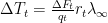$\Delta T_t=\frac{\Delta F_t}{q_t}r_t\lambda_\infty$ of the relationship between stimulus $\frac{\Delta F_t}{q_t}$ and response $\Delta T_t$ was its separating a linear model’s step response into magnitude $\lambda_\infty$ and shape $r_t$ factors. Since by definition $r_\infty=1$ , this makes the relationship between feedback $f$ and equilibrium response value $r_\infty\lambda_\infty=\lambda_\infty$ apparent because $\lambda_\infty=\lambda_0/(1-\lambda_0f)$ , where $\lambda_0$ is the no-feedback value, styled the “Planck climate-sensitivity parameter” in their paper.

“Transience fraction” is the name they gave that shape component $r_t$ : it is a normalized step response. And Roe’s Fig. 6 depicts responses to a $4\,\textrm{W/m}^2$ forcing step. So one might speculate that Monckton et al. obtained their Table 2 transience-fraction values by normalizing those Fig 6 values.

However, that graph contains only one or arguably three curves, whereas Monckton et al.’s Table 2 contains values for five. Rather than explain in response to my consequent inquiry how the authors might have accomplished this loaves-and-fishes feat, Lord Monckton simply stated: “The table was derived from a graph in Gerard Roe’s magisterial paper of 2009 on feedbacks and the climate. Far from obscuring anything, we had made everything explicit.”

Lord Monckton also issued an invitation: “If Mr Born disagrees with Dr Roe’s curve, he is of course entirely free to substitute his own.” I reluctantly accept that invitation, not because I know of any reason to reject (or accept) Dr. Roe’s curves but because the values that Monckton et al. inferred from them are implausible.

Fig. 1 depicts the step responses of which Monckton et al.’s Table 2 are normalized versions. That is, it shows the results of multiplying each row’s entries by the corresponding $\lambda_\infty=\lambda_0/(1-\lambda_0f)$ , where $1/\lambda_0=3.2\,\textrm{W/m}^2/\textrm{K}$ and $f$ is the value their table lists as $f_\infty$ . (Although Monckton et al. also use the notation “ $f_t$ ,” the $f_\infty$ values seem to be the only ones they use, so we will simply use $f$ as our feedback-coefficient symbol.)

Consider that plot’s various values for $t=25$ years. Suppose that 25 years after a $1.0\,\textrm{W/m}^2$ step in forcing we have observed a 0.24 K temperature increase. By consulting that plot, we conclude that the feedback is a modest $0.5\,\textrm{W/m}^2/\textrm{K}$ , implying an equilibrium climate sensitivity of 1.4 K. If the increase were 0.29 K instead, we would infer a rather larger $1.3\,\textrm{W/m}^2/\textrm{K}$ feedback coefficient, which implies a larger equilibrium climate sensitivity, 2.0 K. But if the temperature increase were still greater, 0.31 K, we would infer—no feedback at all. And that implies equilibrium climate sensitivity of only 1.2 K.

How’s that again? A higher current temperature increase implies a lower equilibrium climate sensitivity?

Theoretically, that result is not completely impossible; if you make different system assumptions for different feedback levels, you can get results like that. But it is far from self-evident that the Roe paper from which Monckton et al. purportedly derived their Table 2 dictates so implausible a result. So, to use Monckton et al.’s model but employ more-plausible behavior, we resort to rolling our own version of Table 2.

To that end we will model the system in the manner that Fig. 2 depicts. We use the $H_0(s)$ notation in the forward block as shorthand for its input-output relationship. Dr. Roe said his results came from a model that included diffusion, but for the sake of simplicity we’ll assume a lumped-parameter model. We arbitrarily adopt a third-order relationship between that block’s output $y$ and its input $x$ :

$\frac{d^3y}{dt^3}+q_2\frac{d^2y}{dt^2}+q_1\frac{dy}{dt}=p_2\frac{d^2x}{dt^2}+p_1\frac{dx}{dt}+p_0x$ .

For reasons that will become apparent in due course we adopt the following coefficient values: $q_2=1.7\times 10^{-9}\textrm{sec}^{-1}$ , $q_1=3.2\times 10^{-19}\textrm{sec}^{-2}$ , $p_2=9.8\times 10^{-10}\,\frac{\textrm{K/sec}}{\textrm{W/m}^2}$ , $p_1=4.2\times 10^{-19}\,\frac{\textrm{K/sec}^2}{\textrm{W/m}^2}$ , and $p_0=1.8\times 10^{-29}\,\frac{\textrm{K/sec}^3}{\textrm{W/m}^2}$ .

Fig. 3 depicts the response that such a system exhibits when its input $x$ is a unit step: it asymptotically approaches a linear increase without bound. This is what we would expect of a system that steadily receives heat but sheds no heat in response.

To obtain the step responses for the various levels of feedback in Monckton et al.’s Table 2, we add feedback, as our Fig. 2’s feedback block indicates. This is a simple matter of replacing $y$ with $\Delta T$ and replacing $x$ with $\Delta F + f_{tot}\Delta T$ for respective values of total-feedback coefficient $f_{tot}\equiv f-1/\lambda_0$ :

$\frac{d^3}{dt^3}\Delta T+q_2\frac{d^2}{dt^2}\Delta T+q_1\frac{d}{dt}\Delta T=p_2\frac{d^2}{dt^2}(\Delta F + f_{tot}\Delta T)+p_1\frac{d}{dt}(\Delta F + f_{tot}\Delta T)+p_0(\Delta F + f_{tot}\Delta T)$ .

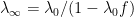
Fig. 4 depicts the solutions to that equation for a unit step in forcing and shows that they approximate all Monckton et al. Table 2 values except the implausible $f=0$ entries. This is not entirely coincidental, since the open-loop equation’s coefficients were so chosen as to make the normalized solution to the corresponding closed-loop equation approximate the entries in one of Table 2’s rows.

The $r_t$ values that correspond to the Fig. 4 solutions take the form

$r_t = 1 - A_1 e^{-t/\tau_1} - A_2 e^{-t/\tau_2} - A_3 e^{-t/\tau_3},\qquad \sum A_i=1.$

For the feedback values in Monckton et al.’s Table 2, the coefficients are as follows, with the $\tau_i$ ’s given in years:

Recall that the total-feedback values $f_{tot}$ we used to obtain those $r_t$ values were sums of the climate-science-style feedback $f$ values and the negative reciprocal $-1/\lambda_0$ of what Monckton et al. call the “Planck climate-sensitivity parameter.” Lord Monckton has <a href=http://wattsupwiththat.com/2015/03/16/where-the-complex-climate-models-go-wrong/#comment-1887123>objected</a> to my having done so: “The misinterpretation – commonplace, but wrong – is in his assumption that the Planck parameter is a feedback just like all the others. No. In fact, it plays a special role in the determination of climate sensitivity, is not summed with the true feedbacks but is, uniquely, instead multiplied by their sum, is separately multiplied by the initial forcing to determine zero-feedback warming, again unlike any of the true feedbacks. . . .”

That objection is largely conceptual rather than substantive. Response curves exactly the same as Fig. 4’s would have resulted if the calculations had been based on the block diagram of Fig. 5 rather than that of Fig. 2. Note that, as Lord Monckton prefers, the feedback-block legend in Fig. 5 is simply $f$ rather than $f-1/\lambda_0$ . Note also that the legend on Fig. 5’s forward block is $H_\lambda(s)$ instead of $H_0(s)$ : Figs. 2 and 5 have different relationships between forward-block output and input. Instead of the open-loop equation given above for $H_0(s)$ , the equation for $H_\lambda(s)$ is the one that results from the above closed-loop equation when $f$ is set to zero: its step response is the solid black curve in Fig. 4.

Now, that response’s $t=\infty$ value is $\lambda_0$ , so the loop gain is indeed $\lambda_0f$ : in a sense, as Lord Monckton says, the “Planck parameter . . . is not summed with the true feedbacks but is . . . instead multiplied by their sum.” But that characterization results merely from the way in which we defined the system and from the level of abstraction we used. The Fig. 5 diagram is merely a higher-level version of Fig. 6, which shows that Fig. 5’s forward block is itself a feedback system. And by the distributive property Fig. 6 is equivalent to Fig. 2, from which we derived our transience-fraction values. So, as far as Monckton et al.’s linearized model goes, little depends on whether the “Planck parameter” is thought of as a feedback quantity: Lord Monckton has objected to form, not substance.

It bears emphasis at this point that Lord Monckton was correct in saying that “in all runs of our model that concerned equilibrium sensitivity (and most of them did) [the transience fraction $r_t$ ] is simply unity”: the relationship between feedback and equilibrium sensitivity does not depend on Monckton et al.’s having gotten the transience fraction right. Moreover, Monckton et al. were modest in their claims for the model, referring to the “rough and ready fashion” in which it represented forcings and feedbacks and pointing out that the model’s use is “narrowly focused on determining the transient and equilibrium responses of global temperature to specified radiative forcings and feedbacks in a simplified fashion.”

The model is advisedly simplified, intended to be simple enough that the authors could commend its use to “those who have no access to or familiarity with the general-circulation models,” just “a working knowledge of elementary mathematics and physics.” And Lord Monckton quite understandably turned down requests for computer code on the basis that users could readily implement the model on a pocket calculator and thereby “be determining climate sensitivity more reliably than the [IPCC] in minutes.”

But the latter feature is the result of the fact that their model $\Delta T_t=\frac{\Delta F_t}{q_t}r_t\lambda_\infty$ simply multiplies the time- $t$ value $\frac{\Delta F_t}{q_t}$ of the stimulus by the time- $t$ value $r_t\lambda_\infty$ of the step response rather than, as would be more conventional, convolving entire time sequences. And, at least as implemented, that feature appears to have resulted from failure to heed Mark Twain’s admonition that we “be careful to get out of an experience only the wisdom that is in it and stop there.”

In response to my observation that, as he put it, “we relied on a model generated by a step-function representing the effects of a sudden pulse in CO2 concentration rather than one in which concentration increases by little and little,” Lord Monckton admitted that they had indeed relied on a step stimulus. But he justified that approach with wisdom he had gotten out of a related experience:

“I had first come across the problem of stimuli occurring not instantaneously but over a term of years when studying the epidemiology of HIV transmission. My then model, adopted by some hospitals in the national health service, overcame the problem by the use of matrix addition, but sensitivity tests showed that assuming a single stimulus all at once produced very little difference compared with the time-smeared stimulus, merely displacing the response by a few years. Similar considerations apply to the climate.”

Even for “determining the transient and equilibrium responses of global temperature,” that experience may have had rather less wisdom than Lord Monckton supposed.

Fig. 7 illustrates transient climate response, i.e., the temperature increase that will have resulted at the time when CO2 concentration has doubled after increasing by 1% per year. The legend in the upper left gives the equilibrium climate sensitivities that Monckton et al.’s Table 2 feedback values imply: it gives the changes in temperature that would ultimately result if that doubled concentration remained in perpetuity. For the corresponding systems, whose step responses Fig. 4 depicts, Fig. 7’s solid curves represent the responses to an instantaneous CO2-concentration doubling, and its dashed curves represent corresponding responses to doubling over about 70 years ( $1.01^{70}\approx 2$ ).

If after the 70 years in which CO2 concentration has doubled we observe the 1.7 K temperature change marked by an “x” on that the plot, then the equilibrium climate sensitivity inferred by the Monckton et al. approach, i.e., from multiplying the current stimulus value by the current step-response value, would be the 3.4 K associated with the solid curve closest to the marked value at 70 years. But the equilibrium climate sensitivity inferred from the more-conventional approach of convolving the stimulus’s derivative with respective step responses would be more like the 12.4 K associated with the closest dashed curve.

There are those who would consider such a difference significant.

Again, this does not mean that the Monckton et al. model is completely unworkable. In particular, I know of no specific problem with the results it gives for the $t=\infty$ , i.e., unity-transience-fraction, case. Moreover, although we have seen that the Monckton et al. approach has significant problems in principle, it would be hard to tell without a more-detailed account of underlying data and assumptions how significantly those problems may have affected the numerical results at which Monckton et al. arrived in practice.

Also, although we have seen that the difference between Monckton et al.’s simple multiplication and the more-accurate, conventional convolution approach can be significant, a simple-multiplication approach may still be justified if the expected forcing trajectories are obliging enough. If the trajectories that the forcings $\frac{\Delta F_t}{q_t}$ follow are expected to be roughly linear, for example, one could adopt $r_t$ values based on a ramp response rather than the step response from which Monckton et al. obtained theirs.

But it is not clear that those conditions apply. In short, Monckton et al.’s model has limitations of which “the user manual for the simple model, bringing it within the reach of all who have a working knowledge of elementary mathematics and physics” omits warnings the reader could have profited from. At the very least, users should exercise caution when they use the model’s $r_t$ values.

0 0 votes

Article Rating

160 Comments

Oldest

Newest Most Voted

Inline Feedbacks

View all comments

Ozziechris

April 1, 2015 1:06 am

Does it matter?

vukcevic

Reply to Ozziechris

April 1, 2015 3:04 am

Feedback formulae don’t, but the variability of the source of energy ( sun ) does !
At the time there was a bit of disagreement about TSI/sunspot role.
The sunspot count for March from SIDC is 38.4 well down on recent peak as you can see HERE .
It appears that the SC24 has peaked about a year ago (see link above)
This is surprisingly as anticipated about some 12 years ago.
Dr. Leif Svalgaard, referring to the rather heretical approach, once said:
“You may turn out to be correct for the wrong reason”
For time being I’ll put stronger accent on ‘correct’ than ‘reason’, case of a conformation bias no doubt.
Well, of course there might be another peak in a year or so, but I strongly doubt that it will exceed one from the early 2014.

Gary Pearse

Reply to vukcevic

April 1, 2015 5:03 am

Vuk, color me impressed!

Joe Born

Reply to Ozziechris

April 1, 2015 4:55 am

What matters is that scientific papers be clear and rigorous.
When I can’t understand a scientific paper, and that happens more often than not, I tend to attribute that to my limitations. No doubt I’m often right.
But I have to say that when I’ve actually taken the time to dig into them I’ve too often found them so marred by latent ambiguities and faulty logic that they couldn’t really have informed anyone, even though many readers have seemed to imagine they’ve been edified. The impression one gets is of a large body of literature largely untouched by human minds. And of large amounts of readers’ time wasted in trying to make sense of things that don’t.
Perhaps an occasional critical review will tend to improve the situation. Or at least that is my hope.

ferdberple

Reply to Joe Born

April 1, 2015 6:05 am

Assuming your numbers are correct, Fig 4 would appear to be a correction to the original, indication that the original f=0 curve was calculated incorrectly.
Fig 7 I have some problem with. The solid lines look like the response one would expect if CO2 doubled today. The dashed lines look like the response one would expect if CO2 doubled over a period of 70 years.
I find it hard to believe that this difference in Fig 7 results from using a discrete approach as compared to a continuous approach. mathematically they should be identical at the limit. We do this all the time on computers for practical reasons, with little difference in accuracy, so long as the problem is well behaved.
The large difference in Fig 7 is to my mind much more likely a result of a difference in assumptions.

ferdberple

Reply to Joe Born

April 1, 2015 11:49 am

ps: the solid lines in Fig look to me like a 100% step size in the first year, with no increase beyond that. A more reasonable assumption is that you would use step sizes of 1/70th of the doubling each year for 70 years. This would return virtually the same curves as the dashes line as derived using the continuous function, with worst case error of about 1/2 year over 70 years.
The actual magnitude of the temp change should be virtually identical, regardless of using a stepped funcion or a continuous function, as per Newton’s, so long as the steps are kept reasonably small.

ferdberple

Reply to Joe Born

April 1, 2015 11:52 am

the advantage of the stepped functions is that it is typically much simpler to work with than the continuous function, with some small loss of accuracy.

Joe Born

Reply to Joe Born

April 1, 2015 4:14 pm

ferdberple: “I find it hard to believe that this difference in Fig 7 results from using a discrete approach as compared to a continuous approach.”
That isn’t the difference. The difference is as you surmise here:
ferdberple:”the solid lines in Fig look to me like a 100% step size in the first year, with no increase beyond that. A more reasonable assumption is that you would use step sizes of 1/70th of the doubling each year for 70 years. This would return virtually the same curves as the dashes line as derived using the continuous function, with worst case error of about 1/2 year over 70 years.”
You’re right; steps of 1/70th cumulatively applied would end up looking just about the same. The reason for the whole step at time t=0 is that it’s the basis for Monckton et al.’s figures.

ferdberple

Reply to Joe Born

April 1, 2015 6:51 pm

You’re right; steps of 1/70th cumulatively applied would end up looking just about the same. The reason for the whole step at time t=0 is that it’s the basis for Monckton et al.’s figures.
==============
You have given a misleading result by stopping Fig 7 at 70 years. If you let Figure 7 run longer, to say 105 years, both the solid lines and the dashed lines should converge to roughly the same values. (In climate terms, 35 years is a few years). What you have demonstrated is what Monckton replied:
“but sensitivity tests showed that assuming a single stimulus all at once produced very little difference compared with the time-smeared stimulus, merely displacing the response by a few years.”

Monckton of Brenchley

Reply to Joe Born

April 3, 2015 2:59 am

I hope that Anthony will in due course print my reply to this post.

Joe Born

Reply to Joe Born

April 3, 2015 9:26 am

ferdberple: “You have given a misleading result by stopping Fig 7 at 70 years. If you let Figure 7 run longer, to say 105 years, both the solid lines and the dashed lines should converge to roughly the same values.”
Not really. Monckton et al.’s approach is to draw an inference from the current forcing value, and their model is based on the theory that this value had prevailed for t years. So the step response would be 130 / 70 times as high as in Fig. 7 unless the forcing increase had obligingly stopped at t = 70.
But you’re right that they’ll come out close in some situations. But you would have to run a check like that of Fig. 7 above to determine whether your situation is one of them. That was my point.

Fernando Leanme

April 1, 2015 1:37 am

I don’t have time to debate the post contents because I’m scouting baseball players in Spain during Easter, and yesterday I found a phenomenom: a Spanish 17 year old with a 106 mph fastball which flies in with a slight rising motion. The kid throws so hard I had to use three catchers in a 30 minute session. And to make this find even more incredible he also runs a 4.2 second 40 yard dash…he can pinch run when he’s not pitching and steal bases at will.
I know the idea of a rising fastball sounds impossible, but we took a high speed video, and it seems the kid puts a super high speed spinning motion on the ball and this creates a vacuum which lifts the ball against the force of gravity with one loop approximation.
For those who are interested in this effect, which I have named the “Juancho”, the renormalization group analysis of mass is performed with the extra initial condition 4λ=g2=(5/3)g′2 for the baseball’s quartic and SU(2)L and U(1)Y gauge coupling constants. This initial condition is introduced in the new scheme of noncommutative differential geometry, but the grand unification of the coupling constants is not realized in this scheme.
I’m signing Juancho to a five year contract and plan to sell him to the NY Mets for $80 million, which may be cheap considering he is going to revolutionize American baseball.

vukcevic

Reply to Fernando Leanme

April 1, 2015 2:36 am

April 1st ?

Fernando Leanme

Reply to vukcevic

April 1, 2015 6:00 am

Yes, it’s April 1, 2015. Are you from the future?

Mashman

Reply to vukcevic

April 1, 2015 6:28 am

I believe so.
I went to his blog, and he compares this pitcher to Sidd Finch.
http://en.wikipedia.org/wiki/Sidd_Finch

vukcevic

Reply to vukcevic

April 1, 2015 6:30 am

Hi
I was referring to:
plan to sell him to the NY Mets for $80 million
regardless of the date,.I wish you success

Beta Blocker

Reply to Fernando Leanme

April 1, 2015 9:05 am

His arm will fall off in 2020, if not sooner.

auto

Reply to Beta Blocker

April 1, 2015 1:28 pm

97% confidence?
Or 97% of scientists are confident?
~Just enquiring . . . . . .
Auto

asybot

Reply to Beta Blocker

April 4, 2015 12:05 am

On April first.

brians356

Reply to Fernando Leanme

April 1, 2015 3:49 pm

Hoax. Spaniards cannot engage in organized baseball in the USA because afternoon games interfere with Siesta.

Dawtgtomis

Reply to brians356

April 1, 2015 7:00 pm

I can delay my nap to watch… what’s the problem here?

Fernando Leanme

Reply to brians356

April 2, 2015 5:18 am

Brian, I’m recruiting these kids from a small fishing village, I picked Juancho from a group of 50 because he was willing to pitch in the afternoon provided he could get up at 10 AM, have a nice breakfast and use social media before going to work. Juancho isn’t as fast as Sidd Finch, but he’s definitely faster than other legends.

Robin Hewitt

April 1, 2015 1:38 am

Surely this is wonderful. Lord Christopher has been complaining for years that the warmistas will not argue science, preferring to argue all kinds of Latin stuff like hominem and absurdum. This looks like he has got his wish. Or have I got it wrong? My brain has been up close and personal with that other latin word “ischaemic” recently and is not what it used to be.

auto

Reply to Robin Hewitt

April 1, 2015 1:29 pm

Robin,
Not, I hope, a silent ischaemic do?
I had to have a stent for mine.
Auto

Robin Hewitt

Reply to auto

April 2, 2015 7:38 am

Ouch, sounds like you are worse off than me. There was no doubting my symptoms, I stood up and went blind in my left eye for 10 minutes. It was quite exciting because I did not know what was coming next.
Robin

Monckton of Brenchley

Reply to Robin Hewitt

April 3, 2015 3:01 am

I am indeed happy that a warmes ta has argued science. I hope my reply will be posted shortly.

Robin Hewitt

April 1, 2015 1:57 am

It’s Greek isn’t it. Oh dear.

son of mulder

April 1, 2015 2:07 am

April stulti est. Non satis tenebrarum.

AlecM

April 1, 2015 2:25 am

Net mean Earth surface IR in self-absorbed GHG bands is exactly zero; the mean 63 W/m^2 is 40 atmospheric window Space and 23 non self-absorbed water vapour bands, absorbed over kilometres.
No CO2 or other main band surface IR means no surface IR thermalisation in the lower atmosphere, no Enhanced GHE. The non-enhanced GHE for all well-mixed GHGs is also kept at exactly zero.
BOTTOM LINE: the paper is a pleasing mathematical curiosity with no bearing on the real atmospheric physics…:o)

azeeman

Reply to AlecM

April 1, 2015 6:35 am

Thank you. Finally a voice of reason.

Konrad.

Reply to AlecM

April 2, 2015 2:18 am

”the paper is a pleasing mathematical curiosity with no bearing on the real atmospheric physics”
Well it certainly has no bearing on atmospheric physics, although I’m not entirely sure why you find it “pleasing”.
Anyone who claims a positive (warming) “climate sensitivity” for CO2 above 0.0ppm is clearly verging on the illiterate regarding radiative physics or fluid dynamics.
My concern is that Viscount Monckton knows he’s got it wrong, but doesn’t care. There seems to be some crazed belief amongst lukewarmers that a Realpolitik “warming but less than we thought” soft landing can be engineered for the hoax. The bottom line is that it can’t. Any attempt to engineer such an exit for the AGW travellers just makes the sceptics involved look incredibly foolish.
Words and flawed mathematical models cannot change physical reality. Those like Monckton who have dabbled in politics cannot perceive the paradigm shift. It no longer matters what the majority think, it now matters what the skilled minority say. The lame scream meeja are no longer the gate keepers of opinion or record. The old rules do not apply. The harsh truth – “there is no net atmospheric radiative GHE on planet ocean, therefore AGW is a physical impossibility” cannot be erased or hidden. The only thing that will be achieved through Monckton’s Realpolitik approach is sceptics looking as stupid as warmulonians.
This is a new age, the age of the Internet. There is no hope of Monckton and his lukewarm ilk herding all sceptic cats behind his “warming but less than we thought” banner. Unless he takes an “AGW is a physical impossibility” stance, he has relegated himself to the losing side.

Monckton of Brenchley

Reply to Konrad.

April 3, 2015 3:03 am

The greenhouse effect is well demonstrated experimentally. The magnitude of the effect of its enhancement on global temperature is, however, questionable. Our paper questioned that magnitude.

steverichards1984

April 1, 2015 2:37 am

An excellent discussion has developed about science and methods involved in climate related research.
Well done, I welcome a suitable response shortly.

Fernando Leanme

Reply to steverichards1984

April 1, 2015 3:38 am

I think the article is bogus, I used the equilibrium climate sensitivity inferred from the more-conventional approach I developed using Kimura´s evolutionary theory and arrived at an equilibrium climate sensitivity below 4 degrees C. And this assumes a 4 watts per m2 positive feedback from clouds between 45 degrees and 65 degrees South latitude. I think the whole post needs to be re-written in a much shorter format and published in the Finnish Academy of Science´s “Lehden noin Roskatiede¨.

Monckton of Brenchley

Reply to steverichards1984

April 3, 2015 3:04 am

I am hoping that my response to this post will be posted shortly.

TonyN

April 1, 2015 2:49 am

“Also, although we have seen that the difference between Monckton et al.’s simple multiplication and the more-accurate, conventional convolution approach can be significant, a simple-multiplication approach may still be justified if the expected forcing trajectories are obliging enough.”
Cymini Sectores?

Michael Spurrier

April 1, 2015 3:27 am

Lord Moncktons birthday today……..or at least it should have been.

Ed Hinton

April 1, 2015 3:53 am

I am no mathematician, but as a lifelong software engineer very familiar with garbage in-garbage out, this bothered me:
“Fig. 3 depicts the response that such a system exhibits when its input x is a unit step: it asymptotically approaches a linear increase without bound. This is what we would expect of a system that steadily receives heat but sheds no heat in response.”
If we are talking about climate sensitivity to CO2, I thought from many other articles that climate sensitivity was logarithmic? If so, then basing a new set of equations on a model that presumes as its basis that the response should by asymptotic to a linear increase does not sound right and it also presupposes that there are no negative feed backs that would increase to compensate.
Perhaps those on this site other that the OP could explain why this should not bother me.

Joe Born

Reply to Ed Hinton

April 1, 2015 4:05 am

I am indeed told that the response to CO2 concentration is logarithmic. But in this case the stimulus we’re talking about is the forcing that results from the CO2-concentration increase. Monckton et al.’s model is linear aft of the CO2-to-forcing step.
Yes, H_0(s) does not include any feedbacks; the feedbacks come when the loop is closed. H_lambda(s) does include what many would call feedback but Lord Monckton prefers not to.
And I agree that radiative feedback must surely increase non-linearly. But we’re talking here about Monckton et al.’s linearized model.

whiten

Reply to Joe Born

April 2, 2015 2:17 am

Hello Joe Born.
I think that the problem actually stands at the point of considering what sensitivity and what response mean in the climate and atmosphere term in relation with CO2 and RF.
As far as I can tell, if I am not wrong, these two aren’t the same.
From my point of view, the atmospheric response to CO2 concentration or CO2 emissions is logarithmic, simply because that is the same relation that atmosphere has with RF.
As the actual logarithmic relation of CO2 variation with RF is too insignificant compared to that of RF and atmosphere, then it can be safely be assumed that the response to CO2 is logarithmic.
The actual response is not to CO2 perse, is actually to energy that atmosphere is subjected to, depending on the energy that RF subjects it too.
The atmospheric response to any warming or cooling it will depend on the RF.
RF dictates to atmosphere when to allow warming or cooling,,,,,,,,,,, CO2 emissions drive the RF.
THere is no direct feedback of atmosphere to the CO2. The CO2 is not sourced from atmosphere.
Unless CO2 considered a climate changer, then there is no any posibility of any feedback either positive or negative in the system above the 0.2C in a climatic term at about above the century mark and further.
The very definition of the CS per a doubling shows the insignificance of the logarithmic relation between CO2 and RF.
Cheers

Monckton of Brenchley

Reply to Joe Born

April 3, 2015 3:11 am

Mr Born assumes, incorrectly, that our model is linear. However, the values of the transience fraction over time may be tuned to simulate any desired response profile, however non-linear, from the original forcing to equilibrium – a point that is made explicitly in our paper. It is, however, regrettable that in formattingg for poblication an appendix that included a further discussion and mathematical representation of non-linear feedbacks was cut immediately before publication.
If anyone wants a copy of the appendix, or of the supplementary matter, email me.

Joe Born

Reply to Joe Born

April 3, 2015 6:56 am

Monckton of Brenchley: “Mr Born assumes, incorrectly, that our model is linear. However, the values of the transience fraction over time may be tuned to simulate any desired response profile, however non-linear, from the original forcing to equilibrium.”
We all know that the climate system being modeled is nonlinear. And I agree that the conversion in Monckton et al.’s model from carbon-dioxide concentration to forcing $\frac{\Delta F_t}{q_t}$ is nonlinear. I’m merely saying that the portion $\Delta T_t=r_t\frac{\lambda_0}{1-\lambda_0f_t}\frac{\Delta F_t}{q_t}$ employed by Monckton et al. to obtain values $\Delta T_t$ of the response from values $\frac{\Delta F_t}{q_t}$ of the stimulus appears linear to me.
If Monckton et al. have arrived at a set of $r_t$ values that make that apparently linear system nonlinear, I hope that Lord Monckton’s response sets it forth with specificity. I will be fascinated to see it, since I have been unable to imagine such a set.

Monckton of Brenchley

Reply to Joe Born

April 3, 2015 7:23 pm

Mr Born does not need “imagination” to work out a non-linear climate-sensitivity curve. Just look at our Fig. 4, which reproduces Roe’s Fig. 6.

Monckton of Brenchley

Reply to Joe Born

April 3, 2015 7:24 pm

And I should add that the IPCC’s own feedback response estimates, insofar as one can derive them from its characteristically obscurantist reports, show a linear response over the first 100-150 years after a forcing.

Joe Born

Reply to Ed Hinton

April 4, 2015 3:14 am

Monckton of Brenchley: “Mr Born does not need ‘imagination’ to work out a non-linear climate-sensitivity curve. Just look at our Fig. 4, which reproduces Roe’s Fig. 6.”
Who knows what Lord Monckton means by “non-linear climate-sensitivity curve”? And who knows whether the model that Roe used to generated his curve was linear? But what we do know is that the model you get by plugging into $\Delta T_t=\frac{\Delta F_t}{q_t}r_t\lambda_\infty$ the Table 2 values Monckton et al. purportedly obtained from that curve is linear.

knr

April 1, 2015 4:09 am

‘users should exercise caution when they use the model’s r_t values.’
has they should with ‘ALL MODELS’ because far from being ‘settled science’ on which massive changes to society and the spending of trillions can be justified . There is much is poorly or even unknown.
One of the differences between the alarmist and sceptics, is that sceptics are able to accept fair criticism of their work and can be honest about how much is really know to be true .

PatrickB

Reply to knr

April 1, 2015 10:43 am

can you point to any calculation or any piece of science that _doesn’t_ involve a model?
if you didn’t use a model to estimate ecs, what _would_ you use?

Todd

Reply to PatrickB

April 1, 2015 12:05 pm

I am currently writing a vision processing algorithm to detect various phenomenon. This algorithm is currently connected to a real live video camera where I (shockingly enough) create the phenomenon in real life.
It is certainly science/engineering. No models necessary.

PatrickB

Reply to PatrickB

April 1, 2015 12:34 pm

your algorithm is, of course, a model.
turning photons into pixels requires a model, the quantum mechanica of how semiconductors function, to turn light waves into electronic signals.
not sure what you mean by “create,” but I highly suspect it uses a model.

Scottish Sceptic

April 1, 2015 4:32 am

One of the funnier articles (and I assume intended – so well done!)
” In short, Monckton et al.’s model has limitations” – yes.
The difference is that these limitations are very obvious and we can all discuss them.
In contrast, the models used to provide IPCC estimates also have limitations, but their unwarranted complexity hides them and prevents proper discussion.
But the proof of the pudding is in the eating.
As far as I know I’m the only person who has said that:
“The Null Hypothesis (Natural Variation) is Consistent with Global Temperatures”
http://www.publications.parliament.uk/pa/cm200910/cmselect/cmsctech/387b/387we32.htm
Which, I would suggest provides a prediction based on Natural variation which would tend toward a “pause”. And guess what? Since that statement in 2009, there has been a pause.
So, I think I’m the only one who’s prediction has been validated (so far).

Gary Pearse

Reply to Scottish Sceptic

April 1, 2015 5:16 am

vukcevic
April 1, 2015 at 3:04 am
He appears to take part of the prize-his forecast was 2004.

vukcevic

Reply to Gary Pearse

April 1, 2015 5:48 am

Hi Gary
Not exactly, Dr. S’s forecast was made public in 2005, my formula was submitted for publication some time in 2003 and published on January 8th 2004, more than a year ahead of the Dr. Svalgaard’s announcement.

ferdberple

Reply to Scottish Sceptic

April 1, 2015 6:25 am

“The public are sick and tired of seeing exaggeration used to “sex up” a situation, creating an atmosphere of fear in order to manipulate us. We saw it with Weapons of Mass Destruction (WMD), and now we see it in global warming.”

Clif Westin

Reply to ferdberple

April 1, 2015 12:50 pm

Or “50 million uninsured”…..

PatrickB

Reply to Scottish Sceptic

April 1, 2015 12:39 pm

the null hypothesis isn’t that natural variability explains modern warming — that’s a hypothesis on its own, and it’s never been proven.
the null hypothesis is that manmade co2 (& othe ghgs) have no relationship to planetary temperatures.
the null hypothesis is rarely, if ever, proved in science, except in a few contrived examples in statistics textbooks.

Chris Hanley

Reply to PatrickB

April 1, 2015 3:13 pm

“the null hypothesis is that manmade co2 (& othe ghgs) have no relationship to planetary temperatures”.
=============================
That statement assumes that manmade CO2 has been observed or is observable.
The null hypothesis is that nothing at all (vis-à-vis the global av. temperature) needs explaining.

Brian H

Reply to Scottish Sceptic

April 2, 2015 2:38 am

Validating a hypothesis is tricky. You have to invalidate every competing one and fail to invalidate your own despite extensive and competent efforts to do so. But my money’s on the Null.

Monckton of Brenchley

Reply to Scottish Sceptic

April 3, 2015 3:20 am

In 2006, when I first wrote about global warming, I predicted that some global warming was to be expected, but on balance not very much. In the eight years 2006-2914′ the world has warmed by 0.07 K.

Monckton of Brenchley

Reply to Monckton of Brenchley

April 3, 2015 3:30 am

Make that 2006-2014. I’m using an iPad.

Alx

April 1, 2015 5:42 am

Well this makes it conclusive that climate models are non-conclusive.
For me the point is not that there is inadequate theoretical proof the models are wrong, there is plenty of empirical evidence they are wrong.
The point is while the climate models are the best that science currently has to offer in describing a model for the climate, discussing the validity of climate models results in relation to forecasting real world events is a non-sequitur. In other words, climate modelers mixed meteorology with delusional visions of global grandeur to create their own peculiar version of a false prophet, the climate model.

vukcevic

April 1, 2015 5:42 am

The CET is back into line after short fall below the 20 year average
http://www.vukcevic.talktalk.net/CET-dMm.htm

emsnews

April 1, 2015 5:59 am

Next: Schrödinger’s cat in a box problem is solved and the world’s temperatures return to ‘normal’ (whatever that is).

Brian H

Reply to emsnews

April 2, 2015 2:44 am

The solution is that observers’ opinions don’t matter; only the cat’s does.

Henry Bowman

April 1, 2015 6:18 am

Thanks for using latex for the equations. I have found MathJax to be easier and produce better-looking results, and all you need is knowledge of Latex.

commieBob

Reply to Henry Bowman

April 1, 2015 11:50 am

Thanks for the tip about MathJax. I’m not sure how Joe Born created his LaTeX but it comes out as alt text for the image of the formula. That means a screen reader will output the formula. My screen reader is Fangs and I can’t get it to play nice with MathJax. Any ideas?

Joe Born

Reply to Henry Bowman

April 1, 2015 5:24 pm

Thanks for the tip. I write it with TexMakerX, which has been working well for me.

Leo Smith

April 1, 2015 6:22 am

In fact step response might be radically different from any of those curves: Consider the step resposne of a high pass filter where feedback is delayed and negative.
gives some suitable curve types. They dont look anything LIKE what is under discussion here…
which goes to show that most people messing with models dont have a clue, and just pick the one that gives them the answers they want.

Solomon Green

Reply to Leo Smith

April 1, 2015 8:42 am

Thanks Leo. Some of us have been saying that for years.
In finance, the Black-Scholes model is still the basis of most models used for valuing derivatives despitei the fact that the principal author, Fisher Black, wrote more than one article poiniting out the “Holes in Black-Scholes” (there were at lest ten) a couple of years after the equation was published. Some years later, both Scholes and Merton won “Nobels” in economics for their work on the equation. (Black had already died, tragically young). And just a few years after that Long Term Capital, the hedge fund of which Scholes and Merton were both directors and investors, collapsed and had to be rescued.

wickedwenchfan

April 1, 2015 6:23 am

I have an even simpler model that is even more effective:
1) I look at Wikipedia’s info on the contribution of CO2 to the Greenhouse effect
2) When I see that it is listed as “between 9% and 27%” of the claimed 33K “extra” heat the greenhouse effect supplies, I laugh at the precise mathematics and wonder which models use 3K as their starting data and which ones use 8K
3) undeterred I make a graph with temperature and CO2 concentration. Using either 3K or 8K ( feel free to use any value inbetween) I make a point at 280ppm and draw a line from zero
4) at 400ppm and 0.8K higher than the last point I make another dot
5) I connect the first dot with the second and make a second line
6) using the artistic side of my brain I make the two lines into a curve if necessary (this will depend on whether you chose 3K or 8K as the temperature value in your first line)
7) I extend the trajectory of my line past 560ppm and onwards towards Venus! (965,000ppm)
8) I laugh at the proponents of CAGW like its April a Fools Day

Gary Pearse

April 1, 2015 6:24 am

Joe Born, perhaps Mark Twain’s remark was even one level more clever. I have taken issue with a number of presentations, such as those of Bob Tisdale, Lord Monckton, this thread, etc. because of assumptions accepted by their authors about IPCC CO2 feedback, the HadCrut, etc temperature records, etc. Now I understand the power in debate of accepting a premise of your ‘opponent’ and then showing what ridiculous things it leads to, logically, but it always leaves me wishing they might take another step. E.g. Bob Tisdale is arguably ‘the’ world expert on ocean heat dynamics and to avoid an extra level of criticism, he illustrates everything using the latest fictitious SSTs and global temp series from the CAGW keepers and creepers of data without comment. There is a limit to the efficaciousness of this continual watering down of one’s thesis. Lord Monckton, too, has used this stratagem and it does cause some heartburn to IPCC chefs.
The problem is we are simply not addressing real climate science this way. We are basically adopting the alarmist’s futures: we are going to hell but it will take longer. A geologist has a harder time than a mathematician in accepting this. I take issue also with the throwing hands up and saying its all chaos and unknowable. We know plenty. We know there is an unbroken chain of life for over a billion years, with some creatures, shellfish, that have even not changed that much. We know that whatever has happened, the earth system has a centering facility that swings it around a few degrees either side of a moderate mean temperature. Even Le Chatelier’s principle that chemical reactions resist influences on them by reacting to counter changes to the existing condition.
http://en.wikipedia.org/wiki/Le_Chatelier%27s_principle .
The universe is governed by negative feedbacks (or it would long ago have gone out in a spectacular manner). Finding a fit with a model that doesn’t recognize this as a controlling feature, or correcting this model is an exercise in futility.

ferdberple

Reply to Gary Pearse

April 1, 2015 6:35 am

The universe is governed by negative feedbacks
========
try and build anything with positive feedbacks and see how long it lasts! no doubt there have been an infinite number of universes with positive feedbacks. and they destroyed themselves before life had a chance to get going. we are here because this specific universe and this specific planet are both ruled by negative feedbacks.
“Any change in status quo prompts an opposing reaction in the responding system.”

Max Photon

Reply to ferdberple

April 1, 2015 8:36 am

Way to damp the conversation 😉

Max Photon

Reply to ferdberple

April 1, 2015 8:42 am

try and build anything with positive feedbacks and see how long it lasts!

That’s why many young people are social train wrecks. They get awarded ribbons and trophies for blinking or having a pulse.
That’s also why Facebook doesn’t have a ‘Dislike’ button; social media is by design a weapon of destruction.
(Someone LIKE this, quickly! It’s been a minute since I’ve had my fix!!!)

Alan McIntire

Reply to ferdberple

April 1, 2015 11:39 am

A-bombs operate on the principle of positive feedbacks. As Gary Pearse pointed out, the feedback factor must be strongly negative, or the climate would have blown up long ago.
http://clivebest.com/blog/?p=2678

whiten

Reply to ferdberple

April 2, 2015 3:43 am

Hello ferdberple.
I generally agree with and appreciate a lot your comments here, but I do at this point disagree with you.
The negative feedback will be a response if there is a positive feedback change in status quo.
The problem is that there is no any such positive feedback observed or measured in the atmosphere in the climatic term. The AGW problem.
The change from status quo appears to be the presiding warming before that of the CO2 emissions.
The increment of RF due to CO2 increment is the means of atmosphere to respond as a system.
It has adopted to it and has evolved that way.
Actually a positive feedback is a lesser change from the status quo of climate than the negative feedback.
Both not observed or measured thus far, as all “climatic constants” still remain so.
While it takes very little to trick the GCMs to project warming due to an artificial positive feedback, it will take much much more to make the same GCMs project a negative feedback.
Cheers

ferdberple

Reply to Gary Pearse

April 1, 2015 6:40 am

a car steering wheel is an excellent example of negative feedback. as you turn the wheel, the wheel tries to turn itself back to the center. imagine now that instead of negative feedback, the steering wheel had positive feedback. as soon as you turned the wheel slightly off center, the wheel would try and force itself more and more off center in the direction of the turn. you would need to fight the wheel to bring it back to center, and if you overshot the wheel would try and force itself in the opposite direction.
how long would such a car last before it drove itself off the road or into another car?

Patrick

Reply to ferdberple

April 1, 2015 7:41 am

That’s not too much to do with the steering wheel, wheels and tyres directly. That’s, mostly, to do with steering geometry, namely camber, castor angles and the ackerman principal. Try putting 56″ wide axles from a Range Rover on a shortened 88″ chassis, you will get amazing tyre scrub when turning full lock! Perfectly OK Off-road! But I get your point. The system is designed, after many years of design and testing, to “straighten out”, or return to a more neutral position with minimal “input” so that you don’t ram someone else or run off the road. Does not always work though!

Tim in Florida

Reply to ferdberple

April 1, 2015 9:45 am

That used to be called manual steering.

Patrick

Reply to ferdberple

April 1, 2015 10:15 am

Nope. The same principals apply. And I have driven many manual and power assisted steered vehicles (PAS). PAS does not alter the performance of the steering geomerty, just makes it “lighter” on the user. The “power assit” bit. Maybe a bit like “PAS” brakes! Or “servo assist”.
Steering (And suspension, and chasiss and power and yeah you get it…before computer control that is) geometry is crucial in vehicle handling. One reason why Lotus, and their cars, were so good! They, eventually, understood automotive geometry. It’s why a Ford Mustang cannot go around a corner like a BMC Mini, or a Lotus Cortina, or a Lotus Escort of the time!

Tom J

Reply to ferdberple

April 1, 2015 12:04 pm

In all due respect (which, from your comments is deserved) I have to disagree with your automobile steering example. It’s primarily a function of the caster geometry in the steering. If one plots a line through the steering pivot axis and all the way to the ground, and this line meets the ground forward of the tire contact patch then the tire will follow that forward pivot point. The steering wheel will not return. Think of the front wheels of a shopping cart. Caster makes cars (and motorcycles) track a straight line at high speed. However, caster increases the effort necessary to steer the car; a somewhat moot point with power steering.

D.J. Hawkins

Reply to ferdberple

April 1, 2015 6:10 pm

This is the phenomenon known as “over-steering”. Read any number of car enthusiast magazines and you are likely to find it a topic of discussion. IIRC, it was more of an issue 40 or so years ago, the last time I spent any effort following the automotive arts. It had its evil twin, “under-steer” that sometimes had to be reckoned with. It was never as extreme as your example, but it did/does exist.

ferdberple

Reply to ferdberple

April 1, 2015 6:22 pm

To understand positive feedback in a car’s steering, try driving backwards at high speed. Coast down a really steep hill so gearing won’t limit your speed. Report back if you survive.
Those movies of people zipping in and out of traffic in reverse with one hand on the wheel? About as realistic as a climate model.

ferdberple

Reply to ferdberple

April 1, 2015 6:30 pm

over-steering
=======
nope. that is caused by unequal front-rear tire slippage at right angles to the direction of travel. over-steer the rear wheels slip sideways faster than the front wheels. under-steer the reverse. of the two, over-steer is typically the most dangerous.
since the front tires wear fastest on most cars, they tend to get replaced while the rear tires do not. This can lead to over-steer, as the front tires will grip while the rear tires slip.

Brian H

Reply to ferdberple

April 2, 2015 2:54 am

Called a “jackknife”.

Tom Trevor

Reply to ferdberple

April 2, 2015 7:48 am

I just got a new boat and trailer, how do I back the thing. I’ve thought watching the tube videos. but somehow this post turned into a better driving lesson than all of those.

Patrick

Reply to ferdberple

April 2, 2015 8:32 am

Ferd, (No disrespect, I always read your name as “Fred”. That’s dyslexia for ya) depends on the steering geomerty again, *and* depends on the drive system. Indepedent front wheel drive will be set up for “toe out” (Plus all the other geometry settings I mentioned). Rear wheel drive, the front wheels will be set up for “toe in” (Plus all the other geometry settings I mentioned). Independent suspension all round and 4×4 (Think Audi Quatro, Subaru Legacy/Impressa etc. Fully independent. Fully adjustable) set up “toe out” at the front, “toe in” at the rear (Plus all the other geometry settings I mentioned). Or two solid “live” axles (Think Landrover. Totally not adjustbale and set at the factory)? The variables, which are all known, cannot be used in your analogy.
The only system that I know of that has no “feedback” at all in steering is something fitted to a 4×4 excavator with a hydraulic ram steering system in the middle. There is no “geometry” and there is no “feedback”.
Driving a vehicle with steering setup for forward motion, CANNOT be driven noramlly (I stress normally) in reverse. The steering system, given the normal geometry of that system, is not “self correcting” in reverse. That’s why it is easy to lose control quickly!
Ignoring centrvical forces, especially with big wheels, ever wonder why bikes and motorbikes can be ridden without holding the handlebars? It’s in part to the “rake” of the front “struts”, or in cars, the castor angle!

Just an engineer

Reply to Gary Pearse

April 1, 2015 7:30 am

It seems to me the IF the CAGW premise was actually true, the reality today would be that the proponents would never have existed to propose it.

Eugene WR Gallun

Reply to Gary Pearse

April 1, 2015 9:35 am

Gary Pearse
“The universe is governed by negative feedbacks (or it would long ago have gone out in a spectacular manner). Finding a fit with a model that doesn’t recognize this as a controlling feature, or correcting that model, is an exercise in futility.”
That sums it all up
I corrected your only mistakes. The second “this” should be “that” and the second “model” should be followed by a comma. Now you are “perfectly” correct.
I just love common sense.
Eugene WR Gallun

Walt D.

Reply to Gary Pearse

April 1, 2015 9:35 am

I’m not sure that Lord Monckton actually believes that you can model the Earth’s climatic system with an 8 parameter model – he is always the first to rub the global warming alarmists noses in it when another month goes by with no appreciable warming. All he demonstrated was that you could do better than the more complex climate system models using similar assumptions and parameters.
In science, some models are simple and the parameters have meaningful interpretations. However, most complex phenomena can not be modeled by a simple equation with a few parameters. (For example, turbulent flow over an aircraft wing – a wind tunnel with actual measurements does a much better job).
In geology and hydrology, statistical methods are often used for interpolation. Nobody claims that the statistical model has any reality – it a just a tool that provides a solution to an otherwise intractable problem. The validity of this type of model (as with any model) lies in its ability to produce accurate predictions.
In this case, all we can say is that within the class of models that use CO2 and a small number of other parameter to model global temperature (whatever that means), Monckton’s model dominates all of the others. As far as I can see, Monckton’s model still predicts a rise in temperature over the last 18 years, even though no appreciable rise has actually occurred.

Monckton of Brenchley

Reply to Walt D.

April 3, 2015 3:41 am

Walt D is right. Every model is a simplification. Every simplification is an analogy. Every analogy breaks down at some point. That is why science based on models’ oredictions can never be settled science.
Yes, our model would predict some warming over the past 18 years – around 0.1-0.2 K. However, most of those years have been in the negative phase of the PDO. That’s why going back to 1990 is better – about half the period is in each phase of the PDO. Our model was spot on when we did that hindcast.

PatrickB

Reply to Gary Pearse

April 1, 2015 10:57 am

The universe is governed by negative feedbacks
================================
not really — the (positive) expansion of the universe is accelerating

Zaphod

Reply to PatrickB

April 1, 2015 11:21 am

Allegedly.
Cosmologists seem to going a bit “epicycles” in recent years.

PatrickB

Reply to PatrickB

April 1, 2015 11:36 am

allegedly? the nobel prize was awarded to that discovery. one of those nobel laureates works on richard muller’s BEST project.

Duster

Reply to PatrickB

April 1, 2015 2:41 pm

Ah, but if you really research the problem of cosmological red shift you will encounter problems ranging from Halton Arp’s photographs (he did not take them) of apparently physically linked high and low red shifts objects (active core galaxies seemingly linked to quasars), through apparent quantization of cosmological red shift to the problem of reconciling it with the laws of thermodynamics. You will also encounter at least four alternatives to the standard model which all are reasonably efficient at articulating the observed phenomena. No, what is really the case is that a so-far useful theory has accounted some observations and the Nobel folks liked it. It is worth noting that Edward Hubble himself rejected Le Maitre’s argument. Cosmology has a great deal in common with climate science, genetics, and other big-ticket research efforts. So do Nobel prizes.

dbstealey

Reply to PatrickB

April 1, 2015 6:46 pm

PatrickB,
I don’t think that strictly qualifies as a feedback.

Brian H

Reply to PatrickB

April 2, 2015 3:00 am

It’s been cancelled. Implosion in a few 10s of billions. So, what’s the point of fixing the climate?

Streetcred

Reply to PatrickB

April 2, 2015 11:11 pm

allegedly? the nobel prize was awarded to that discovery. one of those nobel laureates works on richard muller’s BEST project.

Both Al Gore and Obumbala got Nobel Prezzies … so ? 😉

Monckton of Brenchley

Reply to PatrickB

April 3, 2015 3:44 am

In response to Duster, wasn’t he Erwin rather than Edward Hubble?

Monckton of Brenchley

Reply to Gary Pearse

April 3, 2015 3:28 am

Mr Pearse would enjoy reading our paper. We refer to the remarkable thermostasis of the past 800,000 years. And I have at no point written that we are going to hell in a handcart, only more slowly. It is self-evident from our paper that little anthropogenic warming is likely – less, in fact, than what would be necessary to bring us up to the peak temperature during the last interglacial. That means the rate of warming will be slow, giving flora and fauna plenty of time to adapt.

Salvatore Del Prete

April 1, 2015 7:44 am

An exercise in futility because CO2 and the GHG effect is in response to the climate it does not govern the climate.

Salvatore Del Prete

April 1, 2015 7:47 am

http://jennifermarohasy.com/2013/12/agw-falsified-noaa-long-wave-radiation-data-incompatible-with-the-theory-of-anthropogenic-global-warming-2/
The reality which makes this exercise a more or less wasted effort.

David Wells

April 1, 2015 8:00 am

You might as well use President Mugabe’s dna for all the difference it would make. All we need to know is that it just isn’t warming. Who cares why? Even if we find out it wont make any difference because there is no logical solution. If it warms we fry and if it gets cold we freeze to death but as regards saving the planet think that might just still be here. Can someone explain to me in simple detail why this endless endemic navel gazing really is necessary? Clearly there are just too many people who have nothing better to do with their lives than picking over nano sized detail for no good reason or is that the reason because the climate is so utterly confused and confusing that it allows the more addle brained amongst us to resolve to spend their whole lives pontificating about it because the task that confronts them is endless and sufficiently complicated to allow Obama to enforce his beliefs because you cannot argue with belief, its time to get a life.

Retired Engineer Jim

Reply to David Wells

April 1, 2015 9:57 am

I suspect that a really good reason to be examining everything published about GW / AGW / CAGW / Climate Change / Climate Disruption / Climate Chaos is that the proponents of same are using their “data” and projections to affect policy of the several Governments. The policies are, IMHO, detrimental to the future of our economies and our countries.
It all comes down to the money, large sume of which, again, IMHO, is being wasted.

paqyfelyc

April 1, 2015 8:02 am

bottom line :
climate is chaos and CANNOT be modeled by linear systems
http://wattsupwiththat.com/2015/03/15/chaos-climate-part-1-linearity/
burning carbon mays rise GHG ; or lower them ! after all CO2 is food for plants, and if you give more food to the predators, they mays develop so much that the prey plummet down.
And then rising GHG today may (or not) rise temperature tomorrow. Or cool the planet the day after. or both !
And catastrophe will happen, whatever we do or don’t.
Just be prepared as much as possible.

Bill McCarter

Reply to paqyfelyc

April 1, 2015 9:32 am

Climate is chaos, and cannot be modeled by temperature measurement.

Salvatore Del Prete

April 1, 2015 8:03 am

The optical-density increase raises the effective altitude—and, lapse rate being what it is, reduces the effective temperature—from which the earth radiates into space, so less heat escapes, and the earth warms.
Which data show to be otherwise. My post at 7:47 am Apr 01

cba

Reply to Salvatore Del Prete

April 1, 2015 9:04 pm

lapse rate is a function of conservation of energy. also, while there is more blanketing with increased co2, at stefan’s law level,the emissivity increases causing more radiation from a shell of gas at a given T. The T must drop at this shell as there is not enough new absorbed power to accommodate both the outward and downward increase in radiation. Hence there is a greater differential in T and an increase in conduction/convection. This bs of an effective altitude is non physical. There’s no such thing as a radiating surface at some altitude whose radiation is black body. . Some is from the surface, much of the rest is from cloud tops or wherever there are particulate surfaces that can radiate continuum. higher altitude gas absorption loses its pressure broadening and becomes less effective at affecting broader bands. .

Dodgy Geezer

April 1, 2015 8:12 am

Normal scientific hypotheses propose a mechanism, and them make some predictions by which the validity of that mechanism might be tested. AGW is quite a specific mechanism. There must be lots of ways that it can be tested. A few of these, indeed, came from the alarmists themselves – increased water vapour and the tropospheric hot-spot, for instance.
As far as I know, ALL of these predictions have been proven false. Given that we are spending huge sums of money on this scam, why are more people not calling for a program of hypothesis testing using simple straightforward techniques? It seems to me that modelling will never prove anything, and that when yet another prediction fails the alarmist simply wave their hands and say ‘That doesn’t matter…’ and everyone just stops questioning them…

cba

Reply to Dodgy Geezer

April 1, 2015 9:09 pm

their calculations are based on all worst case scenarios for all variables. they assume that rather than constant relative humidity, it will rise but they also assume that Earth cannot have cloud cover greater than what it is now, around 62%. otherwise they couldn’t have their catastrophe.

Rob F.

April 1, 2015 8:43 am

Just give me the temperature data, the whole temperature data and nothing but the temperature data. The RAW data. From good locations. No “transformation”, “normalization”, “adjusted” or otherwise manipulated. And, for the powers that be, base political decisions on the data, the whole data and nothing but the data.
The data will find you out.
The data will set you free.

Steven Mosher

Reply to Rob F.

April 1, 2015 9:56 am

Ghcn daily.
It’s been there for years.

Salvatore Del Prete

April 1, 2015 8:48 am

http://www.ipcc.ch/publications_and_data/ar4/wg1/en/ch10s10-3-5-6.html
Dodgy another blunder AGW has made.

sabretruthtiger

April 1, 2015 9:06 am

Today is April 1st. When Anthony reposts this on another day I’ll believe it 🙂

Bill McCarter

April 1, 2015 9:30 am

Ceteris paribus, We get lost looking at just one tree in a very big forest, and a very small tree at that. Looking to co2 to being the operator of climate is equivilent to looking to tire pressure as the control system of my car. Temperature is a very lousy proxy for climate, and is used as the “jingling of keys” to distract our attention.

Kevin Kilty

April 1, 2015 9:32 am

Joe Born April 1, 2015 at 4:55 am
What matters is that scientific papers be clear and rigorous…
The impression one gets is of a large body of literature largely untouched by human minds….
Perhaps an occasional critical review will tend to improve the situation.

Thank you for all this effort. I teach a system dynamics course, and so I enjoy seeing some of the concepts of that course applied to an unusual problem.
You have three great quotes in one sort post, here. One thinks that critical reviews would solve many problems — from wasted scientific effort to government malfeasance, but I have found that most people have difficulty understanding a critical review and believers just barge past them anyway. Your second comment about scientific results untouched by human minds is very amusing. Even when some particular topic is well analyzed, there seems always more to investigate. Climate science seems particularly rich in this way.

Joe Born

Reply to Kevin Kilty

April 1, 2015 6:05 pm

Thanks for the kind words.
I take your point that the benefits of critical review tend to be modest. I just like to hope they aren’t non-existent.

Steven Mosher

April 1, 2015 9:54 am

Joe
Nice work.
It’s a shame that William Briggs and Monkton have resorted to the tricks of the team by refusing to clearly explain and document all their steps. Jones used the same trick to thwart Mcintyre.
Please try again and this time send an open letter to all the authors requesting an explanation.

Patrick

Reply to Steven Mosher

April 1, 2015 10:21 am

So only know you see an “issue”?

mothcatcher

Reply to Steven Mosher

April 1, 2015 1:07 pm

Agreed, so they should. Even if the dispute is not fundamental to the main argument. Lord M doesn’t usually duck a challenge, and this is a direct and specific one. However, some of the comments here (esp. Gary Pearse, 6.24 a.m) allude to a broader perspective which gets a lot of points from me. Theoretical math has its limits in this debate.

Monckton of Brenchley

Reply to Steven Mosher

April 3, 2015 3:47 am

Mr Mosher would perhaps benefit from reading our paper before assuming that what Mr Born asserts we have “refused” to explain is not therein explained.

Steven Mosher

Reply to Monckton of Brenchley

April 3, 2015 7:08 pm

post your code

Steven Mosher

April 1, 2015 12:28 pm

“The model is advisedly simplified, intended to be simple enough that the authors could commend its use to “those who have no access to or familiarity with the general-circulation models,” just “a working knowledge of elementary mathematics and physics.” And Lord Monckton quite understandably turned down requests for computer code on the basis that users could readily implement the model on a pocket calculator and thereby “be determining climate sensitivity more reliably than the [IPCC] in minutes.”
This repeats Santer’s argument with McIntryre.
The argument is this.
A. The calculation is so simple that I DONT have to provide it.
So, Monkton has stolen Santer’s trick.
There are two tricks that people like Santer, Jones, and Monkton use.
Trick A: There is IP.. that is the trick is ours to keep
Trick B: It’s trivial.
But if its trivial then there is NO REASON NOT TO SHARE IT.
Here is Santer.. Looks like Monkton went to Santer school
“Dear Mr. McIntyre,
I gather that your intent is to “audit” the findings of our recently-published paper in the International Journal of Climatology (IJoC). You are of course free to do so. I note that both the gridded model and observational datasets used in our IJoC paper are freely available to researchers. You should have no problem in accessing exactly the same model and observational datasets that we employed. You will need to do a little work in order to calculate synthetic Microwave Sounding Unit (MSU) temperatures from climate model atmospheric temperature information. This should not pose any difficulties for you. Algorithms for calculating synthetic MSU temperatures have been published by ourselves and others in the peer-reviewed literature. You will also need to calculate spatially-averaged temperature changes from the gridded model and observational data. Again, that should not be too taxing.
In summary, you have access to all the raw information that you require in order to determine whether the conclusions reached in our IJoC paper are sound or unsound. I see no reason why I should do your work for you, and provide you with derived quantities (zonal means, synthetic MSU temperatures, etc.) which you can easily compute yourself.
I am copying this email to all co-authors of the 2008 Santer et al. IJoC paper, as well as to Professor Glenn McGregor at IJoC.
I gather that you have appointed yourself as an independent arbiter of the appropriate use of statistical tools in climate research. Rather that “auditing” our paper, you should be directing your attention to the 2007 IJoC paper published by David Douglass et al., which contains an egregious statistical error.
Please do not communicate with me in the future.
Ben Santer

Tom Trevor

Reply to Steven Mosher

April 2, 2015 8:03 am

Wow, you’ve gone off the deep end even for you, Mosher. Ben Santer wrote those things, not Monkton. If want to criticize Monkton why not try quoting him?

Steven Mosher

Reply to Tom Trevor

April 3, 2015 7:11 pm

The point is that Monkton is USING Santer’s argument. Santers argument was that he didnt have to supply his code because it was trivial. Monkton is plagarising his argument

Poptech

Reply to Tom Trevor

April 7, 2015 11:42 am

Mosher does this nonsense to try and bully skeptics with his absurd comparisons.

ChipMonk

Reply to Steven Mosher

April 3, 2015 10:22 pm

Mr. Mosher, speaking of “posting” content, can you please provide a full list of 1st-person (yourself with colleagues) research and finding you have created and/or contributed to?
Meanwhile you might find the following interesting: https://pielkeclimatesci.wordpress.com/?s=land+use
Be sure to follow the “older posts” links at the bottom of each page.
Your arguments here might be more helpful without YELLING at people, unless you want to continue using:
Trick C: yell at people until they agree with you.

ChipMonk

Reply to ChipMonk

April 3, 2015 10:43 pm

Mr. Mosher, I was trying to better understand your perspective but I don’t know if this is you:
http://www.populartechnology.net/2014/06/who-is-steven-mosher.html
Please clarify, Thanks.

Poptech

Reply to ChipMonk

April 7, 2015 11:40 am

Yes that is Mosher the non-scientist.

BobG

April 1, 2015 2:24 pm

Joe Born indicated he is a retired lawyer. While I don’t have anything against lawyers, I have found the few I know are “slippery”. They rarely lie outright but some of them are very fond of leading others to come to incorrect conclusions.
It could happen a few ways. Such as making “a request” that comes in the form of a comment to a blog post. You will notice that Joe Born included a link to the entire long thread – but not to a single request. There were many comments on the thread. No one who has a life outside of blogging could have replied to all of the comments and questions before the admin closed comments after a time to that thread.
If Joe Born didn’t email Monckton or contact him outside of the thread, then his comment is without reasonable basis and is deliberately misleading. If he did contact him, he should provide the entire exchange so that others can judge if the request is reasonable, if he waited a reasonable time for an answer and how forthcoming Monckton was.

Joe Born

Reply to BobG

April 1, 2015 5:06 pm

The third sentence of my earlier post said that “the Monckton et al. paper obscures the various factors that should go into selecting [ $r_t$ ],” and the bulk of the post thereafter was directed to what was not clear about that “parameter.” Included was the statement that “In a manner that their paper does not make entirely clear, they inferred the Table 2 relationship from a paper by Gerard Roe.”
I confess my failure to consider the possibility that as a way of eliciting a more-detailed explanation of how Monckton et al. arrived at their $r_t$ more thoroughly this approach would be too subtle. And perhaps I was too hasty in inferring from Lord Monckton’s following statement that it wasn’t: “The table was derived from a graph in Gerard Roe’s magisterial paper of 2009 on feedbacks and the climate. Far from obscuring anything, we had made everything explicit.”
So let me make amends. Here goes:
How did you guys get $r_t$ from the Roe paper?

Phil.

Reply to Joe Born

April 2, 2015 9:35 am

I guess it’s part of the non-existent appendix which Monckton promised to provide?
Monckton of Brenchley January 21, 2015 at 12:39 pm
Try the supplementary material. If the appendix was inadvertently deleted, I’ll send a copy. However, it was only in the appendix, where the system-gain equation for non-linear feedbacks was given, that it was necessary to acknowledge Gerard Roe’s derivation of it: the non-linear form of the equation does not appear elsewhere in the paper. We did try to persuade the editors to send us a copy of the supplementary material as prepared for publication, but we did not receive it.

BobG

Reply to Joe Born

April 2, 2015 9:50 am

If I wanted to get a response from Monckton on your question, I would first of all make sure it is somewhat formal before I indicate that he refused to provide the data. That is, send the authors – Monckton et. all an email. The request then could be very simple, “I’m writing a response to your paper. I can’t figure out how you guys get rt from the Roe paper. Could you show how this was done so that I can reproduce the result?”
If you don’t get a response from a blog comment, it means little. It could be that he allocates X time to blogging and ran out of time or skims the comments and didn’t see your comment or sees a 100 comments and replies to a few of them given his time constraints. But I don’t imagine for a second you didn’t already realize all of the above.
Writing, “Lead author Christopher Monckton turned down my request for further information about how the Table 2 “transience fraction” values in Monckton et al.” at the start of your blog gave me the impression that you had communicated outside of the blog (which would be what would be expected) with Monckton et al and they had refused to provide more details. I can’t imagine personally writing what you did otherwise – because it is a harmful and untrue accusation that should not be made lightly. Then I remembered you were a retired lawyer and then your comment began to make sense in that the motive is probably not about figuring anything out or about science at all.

Phil.

Reply to Joe Born

April 2, 2015 10:43 am

In the responses to his first post concerning his paper monckton usually replied to questions by saying “read the paper”. The following is typical:
Monckton of Brenchley January 21, 2015 at 8:10 am
“Phil.” should read the paper before criticizing it. The derivation of the system-gain relation as it applies to non-linear temperature feedbacks is acknowledged in the appendix in which the derivation appears. My emphasis added.
When challenged about where that appendix could be found monckton responded:
Try the supplementary material. If the appendix was inadvertently deleted, I’ll send a copy. However, it was only in the appendix, where the system-gain equation for non-linear feedbacks was given, that it was necessary to acknowledge Gerard Roe’s derivation of it: the non-linear form of the equation does not appear elsewhere in the paper. We did try to persuade the editors to send us a copy of the supplementary material as prepared for publication, but we did not receive it.
When told that there was no accessible appendix/supplementary information monckton went quiet and we didn’t get the promised copy!
Expecting to get a straight answer from monckton is a forlorn hope I’m afraid.

BobG

Reply to Joe Born

April 2, 2015 12:23 pm

Phil, did you email Monckton or co-authors about not getting the appendix?

Joe Born

Reply to Joe Born

April 2, 2015 6:06 pm

Since the phrases “inquiry” and “turned down” were hyperlinked to the inquiry and the turning down, one is entitled to question either the intellect or the sincerity of someone who professes to have thought the inquiry occurred in a communication outside the blog. In either case little is to be gained by further communication with such a personality.
Others may be interested in knowing, however, that I have in the past actually taken BobG’s proposed approach. A prolific contributor to this site had posted a proof widely hailed as being simple, elegant, and literally irrefutable, whereas I had recognized it as a farrago of latent ambiguities and unfounded assumptions. I went to the trouble of explaining that in detail and e-mailed the explanation to him. No response other than acknowledgment that he had received my missive.
I see little value in repeating such an exercise.

Phil.

Reply to Joe Born

April 2, 2015 6:53 pm

BobG April 2, 2015 at 12:23 pm
Phil, did you email Monckton or co-authors about not getting the appendix?
No he declined to answer and ran away. He knows there is no appendix.

Monckton of Brenchley

Reply to Joe Born

April 3, 2015 3:52 am

Bob G, not Mr Born, is correct. Mr Born did not explicitly ask how we determined our approximate values for the transience frepactiin until so late in the day – and in a startlingly discourteous fashion – that I could not have commented even if I had wanted to. Comments had for some reason been closed on that thread.

Monckton of Brenchley

Reply to Joe Born

April 3, 2015 3:53 am

In response to Phil., if he emails me I will send him the appendix.

Joe Born

Reply to Joe Born

April 3, 2015 8:49 am

“Mr. Born did not explicitly ask how we determined our approximate values for the transience [fraction] until so late in the day – and in a startlingly discourteous fashion – that I could not have commented even if I had wanted to.”
The title of my previous post was, “Reflections on Monckton et al.’s ‘Transience Fraction.’” I said in that post that their paper “obscures the various factors that should go into selecting that parameter.” I further said that Monckton et al. had inferred their Table 2 $r_t$ values from the Roe paper “[in] a manner that their paper does not make entirely clear.”
It taxes even my credulity to believe this left unobvious my belief that Monckton et al.’s determination of the transience fraction $r_t$ wasn’t clear enough. Yet Lord Monckton’s subsequent post did nothing to clarify it.
So I tried the 2×4-between-the-eyes approach: my first comment in the ensuing thread included code that would enable him not only to create this head post’s Fig. 1, in which I illustrated the implausibility of Monckton et al.’s Table 2 values, but also to see the data behind it. Since Lord Monckton was still commenting in that thread two days later, it strikes me as passing strange that he considers that “late in the day.”
In any event, he provided no relevant information. Hence the head post.
I truly had not intended to tax Lord Monckton’s powers of inference so sorely. And I’m grieved that he finds it discourteous that I am thus pressing him for further information. Still, he can avoid having his sensibilities further offended by simply providing the information that the original paper should have contained.

Phil.

Reply to Joe Born

April 3, 2015 9:28 am

Monckton of Brenchley April 3, 2015 at 3:53 am
In response to Phil., if he emails me I will send him the appendix.
Please just post it here so that everyone can have access to it.

Salvatore Del Prete

April 1, 2015 2:47 pm

http://media.al.com/news_huntsville_impact/photo/christy-atmosphere-temps-4fe93b1801f915d6.jpg
What the models predicted which is no where to be found.

Brian H

Reply to Salvatore Del Prete

April 2, 2015 3:12 am

In most radiosonde charts I see a slight cool spot there.
BTW, I gather the HotSpot is supposed to be the signature of any Warming “forcing”, not just AG.

Monckton of Brenchley

Reply to Brian H

April 3, 2015 3:59 am

I had the honor of giving the hot spot its name. Actually, Santer 2003 wrongly assumed the hot spot was a feature unique to anthropogenic warming. Theory would lead us to expect a hot spot whatever the cause of the warming. It’s absence indicates either that there is no warming or that either the surface or the mid-troposphere temperatures are wrongly measured. It is more likely that surface than mid-trop temperatures in the tropics are inadequately measured.

Sturgis Hooper

Reply to Brian H

April 3, 2015 9:31 am

I gave the wet spot its name.
Just kidding…

Dan Pangburn

April 1, 2015 4:42 pm

A simpler proof that CO2 has no significant effect on climate and identification of what actually does cause climate change (95% correlation since before 1900) are at http://agwunveiled.blogspot.com

jim heath

April 1, 2015 5:46 pm

I bought an air conditioner and my climate is perfect

Ed Moran

April 2, 2015 2:03 am

Although the math needed to follow the detail is way beyond me I’ve been encouraged that “Monkton v Born” has enabled a real debate. Now try to imagine this over at Sceptical Science.
Thanks Mr Watts.

Salvatore Del Prete

April 2, 2015 8:30 am

AGW theory has predicted thus far every single basic atmospheric process to be wrong.
In addition past historical climatic data shows the climate change that has taken place over the past 150 years is nothing special and has been exceeded many times over in similar periods of time, in the historical climatic record. I have yet to see data showing otherwise.
Data has also shown CO2 has always been a lagging indicator not a leading indicator. It does not lead the temperature change. If it does I have yet to see data confirming this.
SOME ATMOSPHERIC PROCESSES AND OTHER MAJOR WRONG CALLS.
GREATER ZONAL ATMOSPHERIC CIRCULATION -WRONG
TROPICAL HOT SPOT – WRONG
EL NINO MORE OF -WRONG
GLOBAL TEMPERATURE TREND TO RISE- WRONG
LESSENING OF OLR EARTH VIA SPACE -WRONG
LESS ANTARCTIC SEA ICE-WRONG
GREATER /MORE DROUGHTS -WRONG
MORE HURRICANES/SEVERE WX- WRONG
STRATOSPHERIC COOLING- ?? because lack of major volcanic activity and less ozone due to low solar activity can account for this..
AEROSOL IMPACT- WRONG- May be less then a cooling agent then expected, meaning CO2 is less then a warming agent then expected.
These are the major ones but there are more. Yet AGW theory lives on.

Bernie Hutchins

April 2, 2015 9:49 am

Joe –
Many thanks for the idea from your earlier posts of putting in the capacitor. It adds insight to SEE SOMETHING HAPPENING rather than to see that something HAS HAPPENED.
Three days ago I posted a discussion of your circuit as a nice feedback example:
http://electronotes.netfirms.com/ENWN25.pdf
It is an extension of the figures I posted in a previous thread. In addition, last evening I decided to actually just do it by inverse Laplace transforms. MUCH simpler than I was supposing, and it comes out to two terms – one LP and one HP.
http://electronotes.netfirms.com/JB2.jpg
The LT results are identical to the previous simulations, and offer more insight. Rather than just the final endpoint, we watch it get there.

Joe Born

April 2, 2015 6:03 pm

An interesting aspect of your discussion was the frequency response for a greater-than-unity loop gain: it’s finite. For a purely sinusoidal stimulus, the output remains within limits (in theory). For a sinusoid that doesn’t start until t = 0, though, the response blows up unless (in theory, of course) the phase at t = 0 is just right: in the output a finite-amplitude sinusoid is superimposed on an exponential whose polarity and magnitude depend on the sinusoid’s t = 0 phase.
In practice, of course, the output always blows up, and polarity will be unpredictable because it’s highly sensitive to initial conditions.
By the way, you parsed the amplifier’s step response in a way I hadn’t considered. For myself I first worked it out in Laplace transforms, of course, but I looked at the impulse response as the sum of a Dirac delta of amplitude A (going straight through the amplifier) and a low-pass of amplitude A^2 f / (1 – Af) (following the feedback). Equivalent, of course, but it’s always interesting to look at something from a different angle.

Kevin Kilty

April 3, 2015 9:43 am

Joe Born,
I have had a few days to ponder your article, and I have a couple of points that you might respond to if you care to and have time. First, when I first read the Monckton et al paper, my impression was that they intended this to be a simple procedure of doing forward calculations–i.e. the user could make assumptions about r and q and f, and see what the results would be of Delta T in time. I should perhaps return to their paper and read it again, but that was my point of reference for evaluating their work. Moreover, I also assumed that by using the subscript “t” for r and q they were implying that these might be functions of time.
It makes more sense, perhaps, to see q as a function of temperature, but that renders the problem non-linear again which runs counter to their purpose. Your point regarding convolution of source function and impulse response function is well taken and absolutely correct, but amateurs are not going to program a convolution on a hand calculator. However, a convolution integral results in a function of time; and r, as a general function of time bound by the value 1 as t approaches infinity, is capable of absorbing this. The flaw in Monckton et al is to not discuss this, or to provide guidance on how to go about formulating r so that it approximates use of a convolution integral well.
There was discussion around the internet soon after their paper appeared, with severe criticism about them having made an instantaneous model where temperature changes everywhere instantly–an invalid criticism. I could not see how such criticism arose, but your discussion has helped me understand this better. The parameter r is not intuitive. Point well taken.
Second, in your Figure 4 you show an inverse problem–that of finding the value of some parameter of climatological interest, from temperature observations at particular times. Once again I need to go back and re-read Monckton et al with new eyes, but my understanding of their purpose was that they intend forward calculations. Algorithms that are successful in a forward sense are sometimes just awful in the inverse sense. For instance, my students make temperature measurements of a cooling fin from its root to tip. Some of these students then find a spline function that allows them to calculate temperature at any point on the fin–a forward calculation for which the spline function is a perfectly good model. However, my purpose is for them to find the film coefficient from these measurements–a inverse calculation; and, the spline is worthless for this purpose because none of its parameters relates to film coefficient clearly.
Your Figure 4 gives readers the impression of terrible forward calculation ability, when in fact it shows lousy inverse problem capability if misused. Once again it is the non-intuitive r value, but inverse problems need to be specified and formed quite carefully before rendering a judgement. I found Monckton et al’s paper to be very thought provoking; and I bet it provoked lots of thought in various quarters. Your contribution has clarified some important points.

Joe Born

Reply to Kevin Kilty

April 3, 2015 2:39 pm

Kevin Kilty: “[W]hen I first read the Monckton et al paper, my impression was that they intended this to be a simple procedure of doing forward calculations–i.e. the user could make assumptions about r and q and f, and see what the results would be of Delta T in time.”
That’s my impression, too.
Kevin Kilty: “Moreover, I also assumed that by using the subscript “t” for r and q they were implying that these might be functions of time.”
That’s what I think, too.
Kevin Kilty: “It makes more sense, perhaps, to see q as a function of temperature, but that renders the problem non-linear again which runs counter to their purpose.”
I’m not sure I see why that would make more sense, but, in any case, that possibility hadn’t occurred to me.
Kevin Kilty: “[A]mateurs are not going to program a convolution on a hand calculator. ”
I know that this amateur wouldn’t be inclined to.
Kevin Kilty: “However, a convolution integral results in a function of time; and r, as a general function of time bound by the value 1 as t approaches infinity, is capable of absorbing this.”
True, but only if you know the shape of the stimulus curve in advance.
Kevin Kilty: “The flaw in Monckton et al is to not discuss this, or to provide guidance on how to go about formulating r so that it approximates use of a convolution integral well.”
That’s exactly my point. I attempted in my first post to elicit more details about that function. All I got was a debate; he said they’d already told us everything. My second post’s purpose was to give examples of how that wasn’t necessarily so.
As to the last two paragraphs of your comment, I’m not sure I follow the “forward” and “reverse” nomenclature, but I guess that’s what I get for mucking about in your area. Anyway, in Fig. 4 I was just trying to come up with a more-plausible relationship among the various-feedback systems’ step responses. I don’t follow your abstraction to “finding the value of some parameter of climatological interest.”

BobG

Reply to Joe Born

April 3, 2015 10:36 pm

Being an engineer who has from time to time used feedback equations in my work, and am therefore familiar with the concepts and equations, I found no real issues with Monkton et al.
The intended purpose was give as: “. It is intended to enable even non-specialists to study why the models are running hot and to obtain reasonable estimates of future anthropogenic temperature change.
The model is calibrated against the climate-sensitivity interval projected by the CMIP3 suite of models and against global warming since 1850. Its utility is demonstrated by its application to the principal outputs of the CMIP5 models and to other questions related to climate sensitivity.”
The model is a model used for investigation purposes. I put into a spreadsheet Monckton’s model as it was the simplest and fastest way for me to implement such that I could change the values and create graphs. It took a few minutes to put in the spreadsheet and a while longer to comprehend the variables. It worked as Monckton et al claimed.
Looking at Joe Born’s comments about his quibbles with rt and the Monckton et al model appear as he put it, “largely conceptual rather than substantive.” This is confirmed later when Joe Born wrote, “It bears emphasis at this point that Lord Monckton was correct in saying that “in all runs of our model that concerned equilibrium sensitivity (and most of them did) [the transience fraction r_t] is simply unity”: the relationship between feedback and equilibrium sensitivity does not depend on Monckton et al.’s having gotten the transience fraction right. ”
About rt, “rt is the transience fraction,which is the fraction of equilibrium sensitivity expected to be attained over t years; … In Eq. (1), the delay in the action of feedbacks and hence in surface temperature
response to a given forcing is accounted for by the transience fraction rt.” … “For instance, it has been suggested in recent years that the long and unpredicted hiatus in global warming may be caused by uptake of heat in the benthic strata of the global ocean (for a fuller discussion of the cause of the hiatus, see the supplementary matter). The construction of an appropriate response curve via variations over time in the value of the transience fraction rt allows delays of this kind in the emergence of global warming to be modeled at the user’s will.”
The more times I read Joe Born’s issues with Monckton et al’s use of rt, the stranger it seems. That is because rt behaves from the modeler’s point of view the way I would expect from the discussion. In other words, used in the equation in the described way, it works as described. With respect to whether the transient fraction values that Monckton et al derived were implausible or not that came from Gerard Roe paper’s figure 6, this is not a substantial point. It is rather a small quibble given the purpose of the model and the use of rt in the equation and the fact that as Joe Born noted, the feedback and equillibrium sensitivity does not depend on this fraction being right. A quibble it seems to me that Job Born built up to a huge mountain and turned into what seems to be a mean spirited attack.

Monckton of Brenchley

Reply to Kevin Kilty

April 5, 2015 4:29 am

In response to Mr Kilty, there is in fact quite a bit of discussion in our paper (and more in the appendix) about the representation of the feedback-driven non-linearities in climate response in our model. The transience fraction is the simplest way to handle this. Remarkably, given that feedbacks account for two-thirds of warming in the IPCC’s understanding, time-series graphs of the non-linear evolution of temperature change in the IPCC’s documents are crude and not well explained or justified. We therefore used Roe’s three evolutionary curves as the basis for our table of approximate values.
As to the convolution-vs.-pulse point, we cited in full Roe’s caption making it plain that his curve is based – like many of the curves the general-circulation models and the IPCC produce – on an initial pulse of forcing. We also demonstrate, with worked examples, that the IPCC’s response curve is linear for the first 100 years or so, by which time about half of equilibrium sensitivity will have been attained. And we thrice explain that our values for the transience fraction are approximate. We explicitly state that the user of the model is free to adopt his own values, and almost an entire pages is devoted to discussing these values. Mr Born, in saying we have refused to explain how our values for the transience fraction are obtained, is not only discourteous but erroneous.
As to the question whether convolution-vs.-pulse makes any difference, it is at last agreed even by Mr Born that at equilibrium the value of the transience fraction is by definition unity, convolution or no convolution. And the main thrust of our paper was of course directed towards equilibrium sensitivity.
However, we did also provide worked examples for each of the six RCP concentration pathways to 2100. It will be seen that, in line with our substantial discussion in the paper of the IPCC’s implicit centennial values, we used values 0.5-0.7 for our transience fractions. Now, if one does not determine the convolution integral – which our simple model of course did not do, for we wanted to keep it simple – the consequence is that climate sensitivity will be somewhat overstated in the model. If, therefore, the model is run and shows a significantly lower climate sensitivity than the general-circulation models, then of course a model run on the basis of a convolution interval – which is, of course, time-dependent, as Mr Kilty rightly points out – will show even less climate sensitivity.
Furthermore, the values of individual feedbacks cannot be determined to sufficient precision either empirically or theoretically, nor can we even distinguish the relative magnitudes of forcings and feedbacks. The value of using a single, simple parameter to encompass all of the feedback-driven non-linearities in the climate system response is, of course, that users of the model can readily determine the starting-point (feedback sum zero; system gain 1; transience fraction transient/equilibrium sensitivity); can adopt or not adopt the IPCC’s estimate that half of equilibrium warming occurs after 100 years; and can use our own approximations of the transience fraction as a rough guide. In a simple model, one cannot really do a lot better than that.
The proof of the pudding, of course, will be in the eating. Our model predicts 0.9 K manmade warming by 2100. At present, during a negative PDO phase, the underlying warming rate, which is the rate at which the oceans are warming (if the ARGO measurements were to sufficient precision) is about 0.25 K/century. Of course, much of the CO2 we shall put into the air from now to 2100 is not there yet, and there will be a positive PDO phase from about 2025-2060, so our rough and ready model does seem to be generating predictions that are not by any means unreasonable.
Of course, our best estimate is that negative feedbacks prevail in the climate: otherwise the remarkable thermostasis of the past 810,000 years is rather difficult to explain. In those circumstances, the pulse-vs.-convolution question becomes near-entirely academic. To raise it at all is to require a degree of precision that the resolution of the data and the detail of the theory are in any event unable to support. There are, no doubt, rigorous methods of determining how many angels dance on the head of the average pin, but in the long run your guess is as good as mine. The transience fraction provides a simple and actually quite powerful method of allowing the user of the model to make a coherent guess.

Monckton of Brenchley

April 3, 2015 7:31 pm

Mr Born’s quarrel is with the IPCC, not with me. They have provided no feedback response curves over time, except postage-stamp-sized climate-sensitivity curves – with no data to support them – in AR4 at Fig. 10.26 on p. 803. So we took Roe’s curve and did not worry about convolutions, because the uncertainties in the determination of feedbacks are so large that they swamp such considerations. One can of course, as Mr Born is prone to do, find extreme examples where the difference a convolution and a pulse make a difference. but in the real world the rest of us live in, and over the relatively short timescales we’re concerned with, the difference is unimportant. Using a pulse tends to overstate climate sensitivity, for obvious reasons. So if, even using a pulse, we obtain low climate sensitivities, then if we had used a convolution the sensitivity would have been still lower a fortiori.
It would really help matters if Anthony were able to post my detailed reply to the present post.

Phil.

Reply to Monckton of Brenchley

April 4, 2015 4:52 am

Looking forward to seeing the appendix posted here too.

Monckton of Brenchley

Reply to Phil.

April 4, 2015 4:57 am

If anyone emails me I will send the appendix.

Phil.

Reply to Phil.

April 4, 2015 3:49 pm

Why not post it here?

April 4, 2015 9:20 am

A quibble it seems to me that Job Born built up to a huge mountain and turned into what seems to be a mean spirited attack.
>>>>>>>>>>>>>>>>
Indeed.

Mervyn

April 6, 2015 3:40 am

How many calculations have we now seen regarding climate sensitivity? As nobody can seem to agree about this simple concept in the global warming myth, it is logical to conclude nobody knows the answer.
I go a stage further by saying it is simply impossible to calculate a climate sensitivity value because of the different role CO2 plays in the atmosphere. For example, watch the following NASA video explaining how CO2 is one of two most efficient natural coolants in the atmosphere:
http://www.nasa.gov/mission_pages/sunearth/news/solarstorm-power.html

wpDiscuz

Watts Up With That?

Some updates to the Monckton et al. 'Irreducibly Simple Climate Model'

Like this:

Related

Share this:

Like this:

Related