Guest Essay by Kip Hansen
 “…we should recognise that we are dealing with a coupled nonlinear chaotic system, and therefore that the long-term prediction of future climate states is not possible.”
– IPCC AR4 WG1
Introduction:
The IPCC has long recognized that the climate system is 1) nonlinear and therefore, 2) chaotic. Unfortunately, few of those dealing in climate science – professional and citizen scientists alike – seem to grasp what this really means. I intend to write a short series of essays to clarify the situation regarding the relationship between Climate and Chaos. This will not be a highly technical discussion, but an even-handed basic introduction to the subject to shed some light on just what the IPCC means when it says “we are dealing with a coupled nonlinear chaotic system” and how that should change our understanding of the climate and climate science.
My only qualification for this task is that as a long-term science enthusiast, I have followed the development of Chaos Theory since the late 1960s and during the early 1980s often waited for hours, late into the night, as my Commodore 64 laboriously printed out images of strange attractors on the screen or my old Star 9-pin printer.
PART 1: Linearity
In order to discuss nonlinearity, it is best to start with linearity. We are talking about systems, so let’s look at a definition and a few examples.
Edward Lorenz, the father of Chaos Theory and a meteorologist, in his book “The Essence of Chaos” gives this:
Linear system: A system in which alterations of an initial state will result in proportional alterations in any subsequent state.
In mathematics there are lots of linear systems. The multiplication tables are a good example: x times 2 = y. 2 times 2 = 4. If we double the “x”, we get 4 times 2 = 8. 8 is the double of 4, an exactly proportional result.

When graphing a linear system as we have above, we are marking the whole infinity of results across the entire graphed range. Pick any point on the x-axis, it need not be a whole number, draw a vertically until it intersects the graphed line, the y-axis value at that exact point is the solution to the formula for the x-axis value. We know, and can see, that 2 * 2 = 4 by this method. If we want to know the answer for 2 * 10, we only need to draw a vertical line up from 10 on the x-axis and see that it intersects the line at y-axis value 20. 2 * 20? Up from 20 we see the intersection at 40, voila!
[Aside: It is this feature of linearity that is taught in the modern schools. School children are made to repeat this process of making a graph of a linear formula many times, over and over, and using it to find other values. This is a feature of linear systems, but becomes a bug in our thinking when we attempt to apply it to real world situations, primarily by encouraging this false idea: that linear trend lines predict future values. When we see a straight line, a “trend” line, drawn on a graph, our minds, remembering our school-days drilling with linear graphs, want to extend those lines beyond the data points and believe that they will tell us future, uncalculated, values. This idea is not true in general application, as you shall learn. ]
Not all linear systems are proportional in that way: the ratio between the radius of a circle and its circumference is linear. C =2πR, as we increase the radius, R, we get a proportional increase in Circumference, in a different ratio, due to the presence of the constants in the equation: 2 and π.

In the kitchen, one can have a recipe intended to serve four, and safely double it to create a recipe for 8. Recipes are [mostly] linear. [My wife, who has been a professional cook for a family of 6 and directed an institutional kitchen serving 4 meals a day to 350 people, tells me that a recipe for 4 multiplied by 100 simply creates a mess, not a meal. So recipes are not perfectly linear.]
An automobile accelerator pedal is linear (in theory) – the more you push down, the faster the car goes. It has limits and the proportions change as you change gears.
Because linear equations and relationships are proportional, they make a line when graphed.

A linear spring is one with a linear relationship between force and displacement, meaning the force and displacement are directly proportional to each other. A graph showing force vs. displacement for a linear spring will always be a straight line, with a constant slope.
In electronics, one can change voltage using a potentiometer – turning the knob – in a circuit like this:

In this example, we change the resistance by turning the knob of the potentiometer (an adjustable resistor). As we turn the knob, the voltage increases or decreases in a direct and predictable proportion, following Ohm’s Law, V = IR, where V is the voltage, R the resistance, and I the current flow.
Geometry is full of lovely linear equations – simple relationships that are proportional. Knowing enough side-lengths and angles, one can calculate the lengths of the remaining sides and angles. Because the formulas are linear, if we know the radius of a circle or a sphere, we can find the diameter (by definition), the area or surface area and the circumference.

Aren’t these linear graphs boring? They all have these nice straight lines on them
Richard Gaughan, the author of Accidental Genius: The World’s Greatest By-Chance Discoveries, quips: “One of the paradoxes is that just about every linear system is also a nonlinear system. Thinking you can make one giant cake by quadrupling a recipe will probably not work. …. So most linear systems have a ‘linear regime’ –- a region over which the linear rules apply–- and a ‘nonlinear regime’ –- where they don’t. As long as you’re in the linear regime, the linear equations hold true”.
Linear behavior, in real dynamic systems, is almost always only valid over a small operational range and some models, some dynamic systems, cannot be linearized at all.
How’s that? Well, many of the formulas we use for the processes, dynamical systems, that make civilization possible are ‘almost’ linear, or more accurately, we use the linear versions of them, because the nonlinear version are not easily solvable. For example, Ian Stewart, author of Does God Play Dice?, states:
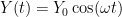
“…linear equations are usually much easier to solve than nonlinear ones. Find one or two solutions, and you’ve got lots more for free. The equation for the simple harmonic oscillator is linear; the true equation for a pendulum is not. The classic procedure is to linearize the nonlinear by throwing away all the awkward terms in the equation.
….
In classical times, lacking techniques to face up to nonlinearities, the process of linearization was carried out to such extremes that it often occurred while the equations were being set up. Heat flow is a good example: the classical heat equation is linear, even before you try to solve it. But real heat flow isn’t, and according to one expert, Clifford Truesdell, whatever good the classical heat equation has done for mathematics, it did nothing but harm to the physics of heat.”
One homework help site explains this way: “The main idea is to approximate the nonlinear system by using a linear one, hoping that the results of the one will be the same as the other one. This is called linearization of nonlinear systems.” In reality, this is a false hope.
The really important thing to remember is that these linearized formulas of dynamical systems –that are in reality nonlinear – are analogies and, like all analogies, in which one might say “Life is like a game of baseball”, they are not perfect, they are approximations, useful in some cases, maybe helpful for teaching and back-of-an-envelope calculations – but – if your parameters wander out of the system’s ‘linear regime’ your results will not just be a little off, they risk being entirely wrong — entirely wrong because the nature and behavior of nonlinear systems is strikingly different than that of linear systems.
This point bears repeating: The linearized versions of the formulas for dynamic systems used in everyday science, climate science included, are simplified versions of the true phenomena they are meant to describe – simplified to remove the nonlinearities. In the real world, these phenomena, these dynamic systems, behave nonlinearly. Why then do we use these formulas if they do not accurately reflect the real world? Simply because the formulas that do accurately describe the real world are nonlinear and far too difficult to solve – and even when solvable, produce results that are, under many common circumstances, in a word, unpredictable.
Stewart goes on to say:
“Really the whole language in which the discussion is conducted is topsy-turvy. To call a general differential equation ‘nonlinear’ is rather like calling zoology ‘nonpachydermology’.”
Or, as James Gleick reports in CHAOS, Making of a New Science:
“The mathematician Stanislaw Ulam remarked that to call the study of chaos “nonlinear science” was like calling zoology “the study of non-elephant animals.”
Amongst the dynamical systems of nature, nonlinearity is the general rule, and linearity is the rare exception.
Nonlinear system: A system in which alterations of an initial state need not produce proportional alterations in any subsequent states, one that is not linear.
When using linear systems, we expect that the result will be proportional to the input. We turn up the gas on the stove (altering the initial state) and we expect the water to boil faster (increased heating in proportion to the increased heat). Wouldn’t we be surprised though, if one day we turned up the gas and instead of heating, the water froze solid! That’s nonlinearity! (Fortunately, my wife, the once-professional cook, could count on her stoves behaving linearly, and so can you.)
What kinds of real world dynamical systems are nonlinear? Nearly all of them!
Social systems, like economics and the stock market are highly nonlinear, often reacting non-intuitively, non-proportionally, to changes in input – such as news or economic indicators.
Population dynamics; the predator-prey model; voltage and power in a resistor: P = V²2R; the radiant energy emission of a hot object depending on its temperature: R = kT4; the intensity of light transmitted through a thickness of a translucent material; common electronic distortion (think electric guitar solos); amplitude modulation (think AM radios); this list is endless. Even the heating of water, as far as the water is concerned, on a stove has a linear regime and a nonlinear regime, which begins when the water boils instead of heating further. [The temperature at which the system goes nonlinear allowed Sir Richard Burton to determine altitude with a thermometer when searching for the source of the Nile River.] Name a dynamic system and the possibility of it being truly linear is vanishing small. Nonlinearity is the rule.
What does the graph of a nonlinear system look like? Like this:

Here, a simple little formula for Population Dynamics, where the resources limit the population to a certain carrying capacity such as the number of squirrels on an idealized May Island (named for Robert May, who originated this work): xnext = rx(1-x). Some will recognize this equation as the “logistic equation”. Here we have set the carrying capacity of the island as 1 (100%) and express the population – x – in a decimal percentage of that carrying capacity. Each new year we start with the ending population of the previous year as the input for the next. r is the growth rate. So the growth rate times the population times the bit (1-x), which is the amount of the carrying capacity unused. The graph shows the results over 30 years using several different growth rates.
We can see many real life population patterns here:
1) With the relatively low growth rate of 2.7 (blue) the population rises sharply to about 0.6 of the carrying capacity of the island and after a few years, settles down to a steady state at that level.
2) Increasing the growth rate to 3 (orange) creates a situation similar to the above, except the population settles into a saw-tooth pattern which is cyclical with a period of two.
3) At 3.5 (red) we see a more pronounced saw-tooth, with a period of 4.
4) However, at growth rate 4 (green), all bets are off and chaos ensues. The slams up and down finally hitting a [near] extinction in the year 14 – if the vanishing small population survived that at all, it would rapidly increase and start all over again.
5) I have thrown in the purple line which graphs a linear formula of simply adding a little each year to the previous year’s population – xnext = x(1+(0.0005*year)) — slow steady growth of a population maturing in its environment – to contrast the difference between a formula which represents the realities of populations dynamics and a simplified linear versions of them. (Not all linear formulas produce straight lines – some, like this one, are curved, and more difficult to solve.) None of the nonlinear results look anything like the linear one.
Anyone who deals with populations in the wild will be familiar with Robert May’s work on this, it is the classic formula, along with the predator/prey formula, of population dynamics. Dr. May eventually became Princeton University’s Dean for Research. In the next essay, we will get back to looking at this same equation in a different way.
In this example, we changed the growth element of the equation gradually upwards, from 2.7 to 4 and found chaos resulting. Let’s look at one more aspect before we move on.

This image shows the results of xnext = 4x(1-x), the green line in the original, extended out to 200 years. Suppose you were an ecologist who had come to May Island to investigate the squirrel population, and spent a decade there in the period circled in red, say year 65 to 75. You’d measure and record a fairly steady population of around 0.75 of the carrying capacity of the island, with one boom year and one bust year, but otherwise fairly stable. The paper you published based on your data would fly through peer review and be a triumph of ecological science. It would also be entirely wrong. Within ten years the squirrel population would begin to wildly boom-and-bust and possibly go functionally extinct in the 81st or 82nd year. Any “cause” assigned would be a priori wrong. The true cause is the existence of chaos in the real dynamic system of populations under high growth rates.
You may think this a trick of mathematics but I assure you it is not. Ask salmon fishermen in the American Northwest and the sardine fishermen of Steinbeck’s Cannery Row. Natural populations can be steady, they can ebb and flow, and they can be truly chaotic, with wild swings, booms and busts. The chaos is built-in and no external forces are needed. In our May Island example, chaos begins to set in when the squirrels become successful, their growth factor increases above a value of three and their population begins to fluctuate, up and down. When they become too successful, too many surviving squirrel pups each year, a growth factor of 4, disaster follows on the heels of success. For real world scientific confirmation, see this paper: Nonlinear Population Dynamics: Models, Experiments and Data by Cushing et. al. (1998)
Let’s see one more example of nonlinearity. In this one, instead of doing something as obvious as changing a multiplier, we’ll simply change the starting point of a very simple little equation:

At the left of the graph, the orange line overwrites the blue, as they are close to identical. The only thing changed between the blue and orange is that the last digit of the initial value 0.543215 has been rounded up to 2, 0.54322, a change of 1/10000th, or rounded down to 0.54321, depending on the rounding rule, much as your computer, if set to use only 5 decimal places, would do, automatically, without your knowledge. In dynamical sciences, a lot of numbers are rounded up or down. All computers have a limited number of digits that they will carry in any calculation, and have their own built in rounding rules. In our example, the values begin to diverge at day 14, if these are daily results, and by day 19, even the sign of the result is different. Over the period of a month and a half, whole weeks of results are entirely different in numeric values, sign and behavior.
This is the phenomena that Edward Lorenz found in the 1960’s when he programmed the first computational models of the weather, and it shocked him to the core.
This is what I will discuss in the next essay in this series: the attributes and peculiarities of nonlinear systems.
Take Home Messages:
1. Linear systems are tame and predictable – changes in input produce proportional changes in results.
2. Nonlinear systems are not tame – changes in input do not necessarily produce proportional changes in results.
3. Nearly all real world dynamical systems are nonlinear, exceptions are vanishingly rare.
4. Linearized equations for systems that are, in fact, nonlinear, are only approximations and have limited usefulness. The results produced by these linearized equations may not even resemble the real world system results in many common circumstances.
5. Nonlinear systems can shift from orderly, predictable regimes to chaotic regimes under changing conditions.
6. In nonlinear systems, even infinitesimal changes in input can have unexpectedly large changes in the results – in numeric values, sign and behavior.
# # # # #
Author’s Comment Reply Policy:
This is a fascinating subject, with a lot of ground to cover. Let’s try to have comments about just the narrow part of the topic that is presented here in this one essay which tries to introduce readers to linearity and nonlinearity. (What this means to Climate and Climate Science will come in further essays in the series.)
I will try to answer your questions and make clarifications. If I have to repeat the same things too many times, I will post a reading list or give more precise references.
# # # # #
The climate seems chaotic, because it depends on changing conditions of space. Many of them can not predict. However DEPENDING exist.
Kip,
I would have said just a little more about linear solution spaces before making the jump to nonlinear ones. The point being that the *solutions themselves* don’t have to look like straight lines for linearity to be present (in the sense we wish to discuss it). For example, suppose that both sin(t) and e^t are solutions to some linear model. Then A sin(t) + B e^t is also a solution, for any values of A and B. I.e. if you saw the system behave like sin(t) in one circumstance, and saw the same system behaving like e^t in another circumstance, you could very easily imagine a new circumstance in which the system would behave a little like both — you could predict the existence of a third circumstance in which it would behave like A sin(t) + B e^t. Your ability to make this kind of linear extrapolation is what goes out the window when your system is nonlinear.
I don’t mean to lecture you, as you are doing a very important service, and I’m sure you know more about nonlinear systems than I do. I only want to make the simple conceptual point that we’re not just talking about *solutions that look like a line.*
Reply to Metric ==> Of course, there are always deeper nuances — linear can be curved as well. Proportionality of outputs to inputs is Lorenz’s key. This is, as explained, a kindergarten introduction 🙂
I bring it up because I can see the following frustrating situation happening. A reader comes away with the impression that “climate modeling is likely to be inaccurate because the modelers are applying a linear model to a nonlinear system.” Then they go and look at a climate model prediction and see something that is definitely not a straight line and think “oh, that criticism must be outdated — they are clearly not just doing linear extrapolations anymore.”
Reply to Metric ==> At some point, we hope that readers can, well….read…. and that giving definitions will help them.
I had trouble finding an example from a homemakers life that would produce a linear, but curved, graph that they would be familiar with.
Thanks for the help.
[Solubility of salt in water, and sugar in water as temperature goes up. .mod]
Thanks again .mod!
Also every harmonic oscillator in existence. A simple harmonic oscillator produces those solutions that are so superimposable because the equation of motion is a linear, second order, ordinary differential equation. When things get nasty/chaotic is when you add a nonlinear driving term and/or when you make the ODE itself nonlinear (which just means that it has terms in it that are powers of the solution or derivatives of powers of the solution being sought with the power in question not being “1”).

 ,
,  , and the right initial conditions. A pure harmonic solution.

 are completely general nonlinear functions of
  . Here one obviously has enormous problems right out of the bat. For one thing, demonstrating that bounded nontrivial solutions exist at all for a given
  combination is a prior chore — there is no reason to think that they will and it is easy to find combinations where they won’t. Indeed, it is probably correct to say that for nearly all combinations they won’t, but this isn’t my own mathematical forte so don’t quote me on that one as an expert.
 are themselves nontrivial functions of t and/or Y and not constants. Things get more complicated but are still linear in 2 and 3 D as well — but I’m not going to do an essay on elliptical PDEs at this particular moment. When you put a function of t in place of the 0 on the right you get inhomogeneous versions of the ODEs and a whole new solution methodology is required, searching for particular solutions to the inhomogeneous equation and adding them to solutions to the associatedc homogeneous equation to get a general solution to an initial value problem. The point is that if one takes an equation like:

 you will get nice, tame, linearized motion where the oscillator eventually oscillates pretty much at frequency
  . Then you’ll hit a regime where you see a double oscillation in steady state. Tweak and there are four oscillation ampltudes in steady state. Tweak and tweak and the system is suddenly chaotic, unpredictable, aperiodic, where teensy changes in the initial conditions lead you to final states that fill the entire phase space of energetically allowable states after the transients have died out.
is the general second order linear homogeneous ODE. Its general solutions are exponentials. For some ranges of A, B and C those solutions are real exponentials. For others they are complex exponentials. Certain linear combinations of complex exponentials are the trig functions cosine or sine. Hence a solution might look like:
for
A general nonlinear second order homogeneous ODE cannot be written down sensibly as there are an infinite number of them. Something like:
might do it, where
This is the way the mathematics of this stuff looks. Nearly all 1-D equations of motion in physics can be put into a form “like” the first equation where superposition works, even when
which describes a rigid pendulum being driven by harmonic driving torque with an arbitrary amplitude and frequency, for some values of the parameters
There are two or three other “classical” simple chaotic oscillators. I have code written for octave/matlab to demonstrate rigid penduli, or there is the double pendulum that is chaotic all on its own, or there is the “Bender bouncer” — an ordinary harmonically driven linear oscillator but with a nonlinear “‘reflection plane” where the mass “bounces” elastically and instantly reverses its momentum. I used to have code for it, and probably still do. The amazing thing is that even thought the systems are or can be quite different, the advent of chaos is the same. Period doubling to chaos, over and over again. Even in finite difference systems instead of ODE solutions, even in iterated maps. Chaos itself is not unstructured and has namable forms and similarities and patterns, at least until its close cousin complexity gets ahold of it and you have (maybe) chaos in N dimensions where N is not a small number. Hard to know exactly what you have in N dimensions.
rgb
I like your writing style.
Reminds me of reading Martin Gardner.
A question I hope you will answer in the next chapter: in a chaotic climate system like Earth, in which there is a new hypothetical man-made warming component being added to the mix (and that is the only change in conditions from before), then maybe the non-linearity of the system will make it impossible to accurately model, but does that mean it is impossible to even make some general conclusions about what will happen? i.e., can we at least say it is likely that the temperature is going to go up (at some unknown rate)? Or is it possible that the temperature could go down?
And how does the discussion of chaos affect the concept of “tipping points”?
Reply to TBraunlich ==> Thank you for the compliment. Martin’s readers of my generation miss him greatly.
I can not answer your question, neither now nor in the next chapter. Why? We simply do not know enough about how the Earth’s climate system works to make even general conclusions at the scale you ask for — will temperatures go up or down? We do not, for instance, know that “there is a new hypothetical man-made warming component being added to the mix (and that is the only change in conditions from before)”. The sun (responsible for the warmth or the Earth, is also changeable. Land use, forest growth and clearing, row farming or pastures, city building, is changeable. Cosmic rays are changeable and unpredictable. Without knowing the system itself, to some pragmatic level of accuracy, we will not be able to make predictions about the future.
“Tipping Points” are theoretical points at which a system will shift from one regime to another, or from one stable state to another stable state. Ice Ages and Inter-glacials are thought of as semi-stable states of Earth’s climate systems, based on past “experience”. Mostly “tipping points” are being used today as scare tactics in the political debate about atmospheric CO2 concentrations.
Linear behavior, in real dynamic systems, is almost always only valid over a small operational range
============
this is fundamental for bikes, cars, boats, planes. All type of vehicles. They have a stability envelop in which their behavior is near linear. Outside that envelope the behavior is non-linear. Thus, what one must master when learning to drive is to keep the vehicle inside the near linear envelop.
predictable systems can be thought of as having a single attractor. A planet orbiting a star is predictable. However, when you add a third body the system becomes chaotic, except in the case where all 3 bodies lie in the same plane.
Chaotic doesn’t mean unpredictable, but it does mean unpredictable for all practical purposes. Given infinite precision and infinite time, you can predict a chaotic system.
Reply to ferdberple ==> Yes and Yes — think of a child learning to ride a bike — pedaling fast enough to get the bike up to speed, while steering close enough to straight, will get the bike on that stable “Look at me Mom, I’d riding a bike!” point.
Thanks, Kip Hansen.
Excellent essay, I will wait for more.
Good essay, Mr. Hansen. I learned about linear functions way back when some where still trying to disprove Ohm’s Law. (Opppppsss,,,showing my age). As a PS….do you consider logarithmic functions as linear or non-linear, or is this discussed in later parts? As for chaotic….sheesh. Sometimes just waking up is chaotic!
Reply to justthinkin ==> I like the pragmatism of Lorenz’s defintion in which one can count on the output being proportional to changes in the input. As you know, graphing a logarithmic on a log scale is linear — a straight line.
Sadly, not a good answer. Linear refers to the ordinary differential equations being solved (or linearity in the difference equations or iterated map equations). Nonlinear ODEs are everything else. See my discussion, with examples, above.
rgb
Enter entropy into the discussion and see where the reality of the climate models end up.
And to Janice and Pamela….there is nothing more chaotic then a rational, logical mind trying to get a FACT across to a “believer”.
Thanks for that. I didn’t expect to follow it, but it was very clear!
Two trivial points, from my own subject.
Ohms law is not actually relevant to the potentiometer example. It’s just confusing ornamentation here. The current and resistance don’t affect the point you make.
And, P = V²2R? (The “2” should be a / . P is V squared OVER R)!
I thought you’d want to know. Typos easily hide in equations.
Cheers,
Zaphod.
Reply to Zaphod ==> Hmmm — I thought this was my Ohm’s Law quote ” As we turn the knob, the voltage increases or decreases in a direct and predictable proportion, following Ohm’s Law, V = IR, where V is the voltage, R the resistance, and I the current flow.”
Ah, found it, you are referring to “voltage and power in a resistor: P = V²2R” — I think you are right, something in the conversion superscripts and subscripts has fouled me up in this quote.
Let me get it right, you are saying it is correctly Power = Voltage squared over Resistance
Right?
[Current = I = Volts/Resistance
Power = I^2 x Resistance = V^2/R = I x V, but only for DC currents.
For AC currents you have to add in the reactance losses and phase changes.
Those are not imaginary losses, but are calculated using imaginary numbers (sq root of -1) ! .mod]
Thanks .mod!
Does this mean that outputs are usually less and never more than a linear view of the inputs would expect? I assume that waste exists, but not a free lunch.
There are two important implications of Chaos theory for this debate that are missed in this article and elsewhere, yet both were well covered by Lorenz.
The first is that it is the non-linearity of the system that often explains its stability.
This is well explained historically (and by one of the sources to this article, Ian Stewart) in the problem of the stability of the solar system. What if it gets a little bump? What about the complex influence of the other revolving planets? Newton solved the problem with the hand of God. Poincare investigated it with the 3-body problem and therein some of the beginnings of the investigation of non-linear systems. This is not equilibrium, not homeostasis, but stable disequilibrium. We do not require equilibrium for stability – this should be a great relief! Nor do we require predictability. This should be obvious with the common usage of the weather/climate distinction.
Even if the precise condition (weather) of a strange attractor at any time is entirely unpredictable by its condition at a previous time, still it is stable, within its range, against perturbation. Yes, there are tipping points, and the degree of perturbation required to push the system over can vary depending on the condition at the time. But, for the solar system, such a perturbation is very unlikely. And even if we do not fully understand the non-linearity of the system under investigation, the longevity of a system in an environment is empirical evidence of its stability. The solar system has been around for a long time and has taken a lot of knocks. Likewise, the amazing stability of the global atmosphere and the climate in terms of such parameters as temperature.
It is an interesting historical fact of this scare that the ‘tipping point’ is emphasized on the alarmist side (Wallace Broecker has a lot to answer for), but also the ‘untamed’ on the skeptic side (surely this is refuted by the old response that we may not be able to predict what the weather will be like on a particular day next summer, but, eg, with our knowledge of ENSO, we may be able to tell you something about the general climatic trend…due to some predictable linearity in the system). A similar emphasis evolved in the Gaia hypothesis. In the mid-70s Lovelock used it to explain and emphasis the stability of the atmosphere in states of disequilibrium — the hypothesis is biospheric self-regulation of a physical system on the analogy of biological systems (eg a cellular organism).
The other important implication relates to the butterfly effect, and what is seen as its teaching of the ‘sensitivity to initial conditions.’ Actually, this understanding of what is going on is very limited. The root problem is about representation of a continuous system in a discrete system. It has deep philosophical implications to do with the very idea of representation of experience. This is often explained historically with Laplace’s idea that the project of science is to strive to represent the world in a model so as to deliver its perfect predictability. Chaos theory declared Laplace’s project over. The teaching for this scare is this: with the collapse of the empirical science of ‘detection’ in the mid-1990s, and so the resort entirely to theoretical modelling (go look at the transition in the work of Barnett, Wigley, Santer etc), we have entered a realm of SiFi. What is truly remarkable historically is how this SiFi is broadly seen across an educated public as continuous with the empirical science from which it evolved.
Extinctions periods are infrequent on Earth, which proves the stability of the system. Life is fragile.
Reply to berniel ==> Yes, of course, one of the attributes of nonlinear systems is the subject called “strange attractors” or sometimes just “:attractors”. In the kindergarten-level May Island squirrel population example above, we see a nonlinear system that is stable at just above 0.6 of the carrying capacity, As long as we don’t change the growth rate, the system settles down at that value — very stable. In fact, there is a whole range of growth rates that produce stable values near 0.6.
Ordinary biology insists that the squirrel population should grow to approximate the carrying capacity — should grow to or close to 1. It does not in our example, and it does not in the real world.
Thank you for bringing up these points, quite valid, but beyond the introductory level of this essay.
Nice to see the subject introduced to give all a feeling for the insoluble problems that chaotic systems create and to make clear, we’re not talking about something rare. I don’t think nonlinearity is the right term, though. Chaotic systems follow neither linear nor nonlinear functions. For forecasting, there is little help to be gotten from any ‘species’ of math once removed from short term linear (or even nonlinear) approximations. Chaos itself would appear to be in a category all its own.
For climate and I’m sure basically all dynamical systems, we have to go with what we do know for long term changes. We do know that chaotic systems have surprisingly neat geometrical expressions – Kip’s classical paired reflected ‘jelly roll’ pattern with two centres (attractors) which seem to be out of bounds for the mad function of chaos. Moreover, the jellyrolls ‘circles’ are of a dimension, finely spaced, the outermost trace of each seeming to be the outer limit for the trace of the function as far as you take it. The space between coils is probably a function of the error of rounding in a parameter or variable. Finally (?) the traces appear to be confined to two planes in the jellyroll case. This is knowing a lot. It would be fun to see what ‘shapes’ we get in functions by rounding off the value of pi in them as we must with a few million iterations of it . Start with two decimal places and then more. Such studies of chaos are more akin to descriptive studies of biological species behavior.
Now climate’s ‘jellyrolls’ are shaped by two attractors, cold and warm and the outer bounds are +/- 5 degrees C as long as the sun is at least roughly constant. Certainly with presently known orbital dynamics, we have the limits of how much energy is being put in and the there must also be a limit to how much it is possible to “magnify” the surface heat on a water planet or how fast we can remove the heat from the system based on this received energy. The detailed weather is a problem beyond a week or so, but I think we can make somewhat confident prognostications from what we know, that we are more likely heading toward another ice age, hopefully far enough into our future to give us time to adapt or head somewhere else for some of us. We are happily being presented with an excellent opportunity for gathering solid data on the likelihood of runaway climate from CO2. Surely another 10 years of no warming will trim CO2’s effect down to insignificant and we can rely on evidence of net negative feedbacks.
The two centers are not attractors. The object itself is the attractor. And it only has this appearance when looked at from just the right angle. Given the right set of parameters and a starting value ‘close’ to the attractor this shape will result over many iterations. It is infinite in length and non-intersecting, which mean non-repeating. What chaotic means is that if you move the starting point a tiny bit (in any direction), the resulting locations after a few thousand iterations will be far apart, but not predictably far apart. And the same change in a different direction will not lead to a predictable result based on the other change. That is sensitive dependence on initial conditions. It also means that tiny errors can be magnified over time (the butterfly effect). There are patterns in chaotic behavior, but they are unusual – hence ‘strange attractor’ – not a point or group of points, but an infinite line, and the ones I have seen were bounded.
This is the kind of article that makes me keep coming back to WUWT over and over again.
Forgive me for making a comment outside of those constraints and maybe off topic.
One of the great things about WUWT is that there are so many contributors that not only know what they are talking about but they are not attempting to deceive. Honesty is refreshing.
(Carry on.)
The discussion in the article and comments is quite interesting. However, some of it gives the impression that linear systems are always approximate desciptions of the real world and in some sense unimportant. Of course, quantum mechanics and quantum field theory are important and they are, as far as we know, perfectly linear. That said, the implications of non linearity for climate predictions are very important. The modelers seem to acknowledge that they cannot predict weather on the 1 month to 10 year scale. Somehow, they think that they can deduce the basic trends on the 10 to 100 year scale. Why do they believe this? Does it have any justification by for example renormalization theory? Can one lump many of the parameters together on the long term?
“Why do they believe this? ”
Their income depends on it.
Reply to Jim Rose ==> “…quantum mechanics and quantum field theory are important and they are, as far as we know, perfectly linear.”
I’d like some quantum physicists to weight in on this idea. Is Mr. Rose’s statement literally true? Or are the equations for the theories linearized out of necessity or for convenience?
I’m a quantum physicist. Quantum mechanics appears to be perfectly linear. I.E. any sum of valid states results in another valid state. In fact, hypothetical nonlinearities in the state space allow some really crazy stuff to happen that seems like it shouldn’t be possible.
However, the time evolution of certain QFT’s is nonlinear, particularly QCD, causing no end of calculational frustrations when applied at low energy when the nonlinearities are biggest.
Metric thanks for the correction. I guess I am starting to show my age — I was thinking of QED. Its still linear isn’t it?
I suppose I should elaborate on my previous statement just a bit. There are a couple different ways you might think about linearity in QM, and it’s easy to get them confused. Let’s describe the state of 1 particle at position A and 0 particles at position B as |1,0>. Similarly, 0 particles at A and 1 particle at B would be |0,1>, and 1 particle at A and 1 particle at B would be |1,1>. Note that |0,1> + |1,0> IS NOT the same as |1,1> — it has a very different interpretation.
Let the time evolution operator be called U.
Now, when people say “quantum mechanics appears to be ABSOLUTELY linear” they mean the following:
If |0,1> and |1,0> are valid states, then so is A |0,1> + B |1,0>. Also, the time evolution of (A |0,1> + B |1,0>) is U(A |0,1> + B |1,0>) = A U |0,1> + B U|1,0>. This is the part that appears to be completely true, to the best of the knowledge of mankind (with people constantly looking for exceptions that would earn them a Nobel Prize).
However, when people say time evolution is nonlinear, they could mean a few subtly different things: They might mean that U|1,1> cannot be regarded as independent operations on the first particle and the second particle seperately — U has to know about both particles to give the right time evolution. This would be the case, for example, if the two particles are charged and applying forces on one another. They also might mean that the interaction force itself is non-linear — this would correspond to the case (as in QCD) where the force-carrying particles (gluons in QCD) also carry their own charges, and thus the exchange of a single force-mediating particle (representing a single “bump” of force) cannot be treated independently from a bunch of other charge interactions.
To Jim Rose:
You’re absolutely right in the sense described above — the state space is linear for every quantum theory we know of. QED is also said to be “linear” in the sense that the force-mediating particles involved (photons) don’t carry a charge, and thus photons can come and go without adding additional computational nightmares to a system of charges you are trying to understand (though, as you mentioned in your first post, renormalization adds yet another layer to the story). QCD is still linear in the state-space sense of the word, but is no longer linear in the force-interaction sense of the word — the mere act of a force occurring between two particles in QCD means that additional charge is introduced and must be taken into account, leading to an infinite series of equally-important terms that make calculating anything “tricky” to say the least, or “horrendous” to be more blunt.
Why do they believe this?
=================
The arguments that climate is predictable revolve around the central limit theorem, the law of large numbers, and the normal distribution.
Many people are familiar with the law of large numbers, and assume that it holds for climate. While a coin toss isn’t predictable in the short term, in the long term it should even out 50-50. However, this doesn’t work for climate. the law of large numbers works when the system under study has a constant average and deviation. like a coin or a pair of dice. this can be readily shown from the paleo records to be false for climate. the law of large numbers doesn’t apply to climate.
The central limit theorem is a more general case of the law of large numbers, and it tells us that if we sample climate randomly we should get a normal distribution. the normal distribution is quite important, because it allows us to make all sorts of statistical predictions using mathematics developed originally to try and beat the casinos. unfortunately the central limit theorem doesn’t apply for a power series distribution such as climate.
when one looks at climate it becomes apparent that temperature for example is a fractal distribution. When you look at a temperature graph, unless the scale is written underneath, you cannot tell if you are looking at 10’s, hundreds, thousands, or millions of years. When you compare this to a coin toss, you immediately see the difference. The coin toss smooths out the longer the time. Climate doesn’t.
It is the fractal distribution in climate that makes it unpredictable at scale, because we currently lack the mathematics to deal statistically with fractals. Much the same time as chaos theory, they give us a view into infinity we did not suspect existed.
http://en.wikipedia.org/wiki/Benoit_Mandelbrot#/media/File:Mandel_zoom_08_satellite_antenna.jpg
“While in the short term a coin toss isn’t predictable in the long term it should be”. The word “should” is the key word here, because in reality it isn’t. The evidence for this are the many gamblers recording the statistical anomalies on Red, Black, Odd, Even, 1-18 and 19-36 of a roulette table and betting on the option that is at 45% over thousands of spins.
The paradox is that the wheel has no memory of what it did before and the long term trend is meaningless even in this simple “coin toss” scenario. The bank accounts of the people who believe otherwise stand testament to this.
It is of course the number zero that, also paradoxically, does give the house a long term advantage. My understanding of the warmists augment is that the IR absorbtion qualities give their climate models a “house edge”. An extra input that skews the odds in favour of warming over the long term.
Reply to wickedwenchfan ==> In my experience with gamblers, it is their “magical thinking” that gives the House the edge — the “zero” and “double zero” only change the odds. I have a brother who spent years working out a “scientific system” to win at blackjack. It was real and gave him a something <1% advantage — a real statistical advantage but one that could not be taken advantage of — as the gambler can not and will not mechanically follow a system, he always gets and follows a hunch. In the normal course of play, such a small advantage leads to one losing his stake long before his advantage appears as a reality in his pile of chips.
I did know one successful gambler — I was counseling him on personal ethics. I couldn't for the life of me figure out how he managed to not only survive, but get wealthy as a professional poker player in the casinos (not like today's Professional Gambler circuit). I finally got it, "It's simple," he says "I cheat."
This gets a bit beyond my math ability, but if I understand the concept, a non-linear system need not be chaotic, but any two or more coupled non-linear systems cannot be non-chaotic. Like the three body problem. Is that correct?
No. The critical part is that a feedback must amplify distortions, i.e. shift state information to the left over system iterations (when encoding the state vector of the system as a digital representation). You can have nonlinear feedback systems that dampen disturbances, those will not show chaotic behaviour.
Thanks
It might not be possible to answer my query. I took one stats class about 25 years ago while in business school. By the second or third lecture, I realized how terribly deficient my education had been for lack of real statistics training. Alas and alack, I didn’t have the time to take more, and now it’s been quite a while since even that one class.
I’ve read Doug Keenan’s criticism of the IPCC reports, and my ignorance both forthrightly admitted and (I think) notwithstanding, it struck me as powerful and possibly even definitive. However, the rebuttals seemed to criticize Keenan for being over-linear (?) in his analysis. Can anyone here with the gift of clarity and the patience to deal with an intelligent yet sadly ignorant non-specialist post about how chaos and linearity might validate or invalidate Keenan’s work?
If you do it, please go slowly and minimize the jargon (or at least define your terms). Ignorance isn’t stupidity; with some help, I’ll get it. The alternatives are either not to ask or to pretend I know what I don’t know. Thanks in advance.
Reply to Jake J ==> I am not familiar with Keenan’s work. Perhaps one of our reader’s more involved in the issue can help you here.
from 2013 –
http://wattsupwiththat.com/2013/10/30/statistical-analyses-of-surface-temperatures-in-the-ipcc-fifth-assessment-report/
Guest essay by Douglas J. Keenan with link to his full critique (pdf)
I haven’t been all the way through it yet, but could help Jake J.
I will go through it . . .
I’ve read Keenan’s stuff, and the rebuttals. I’m trying to figure out where this article fits in. I’m just not well versed enough to know, hence my request of others here. This is a high-quality site, and I figured someone would know.
Kip, a couple links if you want to read Keenan. His stuff was some of the first anti-AGW stuff I found when I decided to re-examine the issue last year. Definitely got my attention, because it looked like he demolished the IPCC. But I always want to read both sides of an argument; this one’s hard if you’re not well versed in stats.
http://www.informath.org/media/a41.htm
http://quantpalaeo.wordpress.com/2013/05/28/testing-doug-keenans-methods/
Reply to Bubba Cow and Jake ==> Thanks for the links.
Thanks, Kip. I realize you have lots of fish to fry. You might not have the time to lead my “over the hills and through the woods to grandmother’s house.” If anyone else can, I’d be genuinely grateful.
Both the chaoticity and the complexity of the climate system argue strongly that the central equation of the current climate paradigm is not true. This is the uber-linear claim that changes in surface temperature are a linear function of changes in forcing. In particular, the temperature change is said to be the change in forcing times an imaginary constant called the “climate sensitivity”, as simple a linear relationship as one can imagine.
I have never seen any reason, either practical, observational, or theoretical, to believe that temperature is a linear function of forcing.
w.
Reply to willis ==> “I have never seen any reason, either practical, observational, or theoretical, to believe that temperature is a linear function of forcing.”
….and nor are you likely to ever see such reasons. And, yes yes and yes, it is the chaotic and the complexity of the Climate System that tells us that such a relationship does not, can not, exist.
Locally, temperature is a function of input heat (and loss) in a manner that might be appropriately linear. But what if the forcing itself is nonlinear / chaotic?
Exactly. It bothers my last living brain cell to see a climate anything graph with a linear trend. The temperature average is not linear, over time the so called average (falsely referred to by some as normal) is nonlinear.
Willis, I completely agree. Temperature rise is not the force. Especially not on the scale that warmists adhere to. Why? Because the oceanic/atmospheric conditions that lead to temperature changes are powerful entities. The energy available to drive these powerful entities this way or that just is not there in the tiny amount of temperature increase realized by additional anthropogenic CO2, thus additional anthropogenic water vapor, added to the atmosphere.
Kerry is a doofus!
…and ‘warrenlb’ might be an alias.
Thanks Kip. Doing great. I realize that you’re planning on moving into climate later and I appreciate that. Sorry I was unavailable a ways back when you were leading a discussion on accuracy, errors . . . Hope we’ll get back to that.
Still I think it may be useful to include a very general sense of data into the function discussion and a bit on the business of going beyond (and even within) the boundaries of your function –
Regardless of the function, assuming it is known (that’s a very big assumption), the information (data) we deal with are scores for that function that are measured, adjusted or modeled and that are also generally time series forms or from some other incremental variable.
There is a delta period between each datum and the next and perhaps some frequency with which the data are produced.
There have been aggressive efforts to both extrapolate and interpolate from those data. The extrapolation bit is guessing the future, of course, and completely questionable for anything including climate prediction or hind casting. Think that if you gain 10 pounds, you’ll be an inch taller.
But there have also been extremely dubious “predictions” with interpolation. Some have claimed this can produce greater “accuracy” within the data which, I recall, they were calling downscaling. No matter how you connect the consecutive dots (lines, swirls), there is no data between those dots – only a range of guesses – but no real information.
As an example that downscalers were actually trying to pull off –
Taking time series weather imagery from (I can’t remember exactly where this was in the US) say Boston and New York City and downscaling that to show what must have been the weather in Hartford. In the data, there simply is no Hartford.
So we not only have to deal with whatever math functions, but also keep a clear eye on the ball. Even if you have the right function, it takes great care to interpret those data and we have already seen many imaginative efforts to make interpretations, which usually have agendas.
Kip,
Perhaps you will appreciate what I recently wrote on a different thread.
* * * * *
Have you ever played with the logistic equation using a spreadsheet? It’s absolutely fascinating that such a simple device can produce so much interesting complexity. If you haven’t done so, I highly recommend it. (It’s awesome to share the experience with young people!)
In particular, the input points that produce intermittency are a marvel. The output graph will display rhythmic patterns that give way to chaos, and then back to rhythmic … great stuff.
I think those infected with climate rabies would do well to take a shot of the logistic equation to at least ease the symptom of frothing.
Reply to Max Photon ==> Yes, of course, that’s how one cuts one’s teeth in Chaos Theory!
Excel is a terrific tool for repeating (copy and paste down a column) the iterative formula. I use ploy.ly online plotting service to make the graphs, uploading the excel files from by machine.
More on this in the next installment.
Kip wrote:
Oh that takes me back! I would wait for eons for the tiniest portions of Julia sets to print. It was SO EXCITING to see even a little bit of ‘roughness’ appear on the paper.
It’s somewhere between sad and comical that Mandelbrot four-wheel-drove over Gaston Julia (and Pierre Fatou) to stake his claim on fractals. It’s kind of like Gore’s discovering the internet.
except gore discovered the internet only 5 years ago
Two books I would enthusiastically add to the reading list are:
The Art of Modeling Dynamic Systems: Forecasting for Chaos, Randomness and Determinism
http://www.amazon.com/The-Art-Modeling-Dynamic-Systems/dp/0486462951
and
The Self-Made Tapestry: Pattern Formation in Nature
http://www.amazon.com/Self-Made-Tapestry-Pattern-Formation-Nature/dp/0198502443/ref=sr_1_1?s=books&ie=UTF8&qid=1426455838&sr=1-1&keywords=the+self+made+tapestry
Max, have not read either. Homework accepted.
They are two of my favorite books.
Chaos knows not even itself, let alone that the universe exist due to chaos’s outputs.
Man kinds input into chaos is to small to measure by any means let alone man kinds puny input into the mix by driving a car to work.