This exercise in data analysis pins down a value of 1.8C for ECS.
Guest essay by Jeff L.
Introduction:
If the global climate debate between skeptics and alarmists were cooked down to one topic, it would be Equilibrium Climate Sensitivity to CO2 (ECS) , or how much will the atmosphere warm for a given increase in CO2 .
Temperature change as a function of CO2 concentration is a logarithmic function, so ECS is commonly expressed as X ° C per doubling of CO2. Estimates vary widely , from less than 1 ° C/ doubling to over 5 ° C / doubling. Alarmists would suggest sensitivity is on the high end and that catastrophic effects are inevitable. Skeptics would say sensitivity is on the low end and any changes will be non-catastrophic and easily adapted to.
All potential “catastrophic” consequences are based on one key assumption : High ECS ( generally > 3.0 ° C/ doubling of CO2). Without high sensitivity , there will not be large temperature changes and there will not be catastrophic consequences. As such, this is essentially the crux of the argument : if sensitivity is not high, all the “catastrophic” and destructive effects hypothesized will not happen. One could argue this makes ECS the most fundamental quantity to be understood.
In general, those who are supportive of the catastrophic hypothesis reach their conclusion based on global climate model output. As has been observed by many interested in the climate debate, over the last 15 + years, there has been a “pause” in global warming, illustrating that there are significant uncertainties in the validity of global climate models and the ECS associated with them.
There is a better alternative to using models to test the hypothesis of high ECS. We have temperature and CO2 data from pre-industrial times to present day. According to the catastrophic theory, the driver of all longer trends in modern temperature changes is CO2. As such, the catastrophic hypothesis is easily tested with the available data. We can use the CO2 record to calculate a series of synthetic temperature records using different assumed sensitivities and see what sensitivity best matches the observed temperature record.
The rest of this paper will explore testing the hypothesis of high ECS based on the observed data. I want to re-iterate the assumption of this hypothesis, which is also the assumption of the catastrophists position, that all longer term temperature change is driven by changes in CO2. I do not want to imply that I necessarily endorse this assumption, but I do want to illustrate the implications of this assumption. This is important to keep in mind as I will attribute all longer term temperature changes to CO2 in this analysis. I will comment at the end of this paper on the implications if this assumption is violated.
Data:
There are several potential datasets that could be used for the global temperature record. One of the longer and more commonly referenced datasets is HADCRUT4, which I have used for this study (plotted in fig. 1) The data may be found at the following weblink :
http://www.cru.uea.ac.uk/cru/data/temperature/HadCRUT4-gl.dat
I have used the annualized Global Average Annual Temperature anomaly from this data set. This data record starts in 1850 and goes to present, so we have 163 years of data. For the purposes on this analysis, the various adjustments that have been made to the data over the years will make very little difference to the best fit ECS. I will calculate what ECS best fits this temperature record, given the CO2 record.

Figure 1 : HADCRUT4 Global Average Annual Temperature Anomaly
The CO2 data set is from 2 sources. From 1959 to present, the Mauna Loa annual mean CO2 concentration is used. The data may be found at the following weblink :
ftp://aftp.cmdl.noaa.gov/products/trends/co2/co2_annmean_mlo.txt
For pre-1959, ice core data from Law Dome is used. The data may be found at the following weblink :
ftp://ftp.ncdc.noaa.gov/pub/data/paleo/icecore/antarctica/law/law_co2.txt
The Law Dome data record runs from 1832 to 1978. This is important for 2 reasons. First, and most importantly, it overlaps Mauna Loa data set. It can easily be seen in figure 2 that it is internally consistent with the Mauna Loa data set, thus providing higher confidence in the pre-Mauna Loa portion of the record. Second, the start of the data record pre-dates the start of the HADCRUT4 temperature record, allowing estimates of ECS to be tested against the entire HADCRUT4 temperature record. For the calculations that follow, a simple splice of the pre-1959 Law Dome data onto the Mauna Loa data was made , as the two data sets tie with little offset.

Figure 2 : Modern CO2 concentration record from Mauna Loa and Law Dome Ice Core.
Calculations:
From the above CO2 record, a set of synthetic temperature records can be constructed with various assumed ECS values. The synthetic records can then be compared to the observed data (HADCRUT4) and a determination of the best fit ECS can be made.
The equation needed for the calculation of the synthetic temperature record is as follows :
∆T = ECS* ln(C2/C1)) / ln(2)
where :
∆T = Change in temperature, ° C
ECS = Equilibrium Climate Sensitivity , ° C /doubling
C1 = CO2 concentration (PPM) at time 1
C2 = CO2 concentration (PPM) at time 2
For the purposes of this test of sensitivity, I set time 1 to 1850, the start of the HADCRUT4 temperature dataset. C1 at the same time from the Law Dome data set is 284.7 PPM. For each year from 1850 to 2013, I use the appropriate C2 value for that time and calculate ∆T with the formula above. To tie back to the HADCRUT4 data set, I use the HADCRUT4 temperature anomaly in 1850 ( -0.374 ° C) and add on the calculated ∆T value to create a synthetic temperature record.
ECS values ranging from 0.0 to 5.0 ° C /doubling were used to create a series of synthetic temperature records. Figure 3 shows the calculated synthetic records, labeled by their input ECS, as well as the observed HADCRUT4 data.

Figure 3: HADCRUT4 Observed data and synthetic temperature records for ECS values between 0.0 and 5.0 ° C / doubling. Where not labeled, synthetic records are at increments of 0.2 ° C / doubling. Warmer colors are warmer synthetic records.
From Figure 3, it is visually apparent that a ECS value somewhere close to 2.0 ° C/ doubling is a reasonable match to the observed data. This can be more specifically quantified by calculating the Mean Squared Error (MSE) of the synthetic records against the observed data. This is a “goodness of fit” measurement, with the minimum MSE representing the best fit ECS value. Figure 4 is a plot of MSE values for each ECS synthetic record.

Figure 4 : Mean Squared Error vs ECS values. A few ECS values of interest are labeled for further discussion
In plotting, the MSE values, a ECS value 1.8 ° C/ doubling is found to have the minimum MSE and thus is determined to be the best estimate of ECS based on the observed data over the last 163 years.
Discussion :
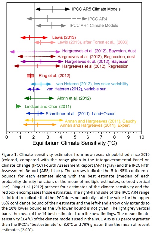
A comparison to various past estimates of ECS is made in figure 5. The base for figure 5 comes from the following weblink :
http://www.cato.org/sites/cato.org/files/wp-content/uploads/gsr_042513_fig1.jpg
See link for the original figure.

Figure 5 : Comparison of the results of this study (1.8) to other recent ECS estimates.
The estimate derived from this study agrees very closely with other recent studies. The gray line on figure 5 at a value of 2.0 represents the mean of 14 recent studies. Looking at the MSE curve in figure 4, 2.0 is essentially flat with 1.8 and would have a similar probability. This study further reinforces the conclusions of other recent studies which suggest climate sensitivity to CO2 is low relative to IPCC estimates .
The big difference with this study is that it is strictly based on the observed data. There are no models involved and only one assumption – that the longer period variation in temperature is driven by CO2 only. Given that the conclusion of a most likely sensitivity of 1.8 ° C / doubling is based on 163 years of observed data, the conclusion is likely to be quite robust.
A brief discussion of the assumption will now be made in light of the conclusion. The question to be asked is : If there are other factors affecting the long period trend of the observed temperature trend (there are many other potential factors, none of which will be discussed in this paper), what does that mean in terms of this best fit ECS curve ?
There are 2 options. If the true ECS is higher than 1.8, by definition , to match the observed data, there has to be some sort of negative forcing in the climate system pushing the temperature down from where it would be expected to be. In this scenario, CO2 forcing would be preventing the temperature trend from falling and is providing a net benefit.
The second option is the true ECS is lower than 1.8. In this scenario, also by definition, there has to be another positive forcing in the climate system pushing the temperature up to match the observed data. In this case CO2 forcing is smaller and poses no concern for detrimental effects.
For both of these options, it is hard to paint a picture where CO2 is going to be significantly detrimental to human welfare. The observed temperature and CO2 data over the last 163 years simply doesn’t allow for it.
Conclusion :
Based on data sets over the last 163 years, a most likely ECS of 1.8 ° C / doubling has been determined. This is a simple calculation based only on data , with no complicated computer models needed.
An ECS value of 1.8 is not consistent with any catastrophic warming estimates but is consistent with skeptical arguments that warming will be mild and non-catastrophic. At the current rate of increase of atmospheric CO2 (about 2.1 ppm/yr), and an ECS of 1.8, we should expect 1.0 ° C of warming by 2100. By comparison, we have experienced 0.86 ° C warming since the start of the HADCRUT4 data set. This warming is similar to what would be expected over the next ~ 100 years and has not been catastrophic by any measure.
For comparison of how unlikely the catastrophic scenario is, the IPCC AR5 estimate of 3.4 has an MSE error nearly as large as assuming that CO2 has zero effect on atmospheric temperature (see fig. 4).
There had been much discussion lately of how the climate models are diverging from the observed record over the last 15 years , due to “the pause”. All sorts of explanations have been posited by those supporting a high ECS value. The most obvious resolution is that the true ECS is lower, such as concluded in this paper. Note how “the pause” brings the observed temperature curve right to the 1.8 ECS synthetic record (see fig. 3). Given an ECS of 1.8, the global temperature is right where one would predict it should be. No convoluted explanations for “the pause” are needed with a lower ECS.
The high sensitivity values used by the IPCC , with their assumption that long term temperature trends are driven by CO2, are completely unsupportable based on the observed data. Along with that, all conclusions of “climate change” catastrophes are also completely unsupportable because they have the high ECS values the IPCC uses built into them (high ECS to get large temperature changes to get catastrophic effects).
Furthermore and most importantly, any policy changes designed to curb “climate change” are also unsupportable based on the data. It is assumed that the need for these policies is because of potential future catastrophic effects of CO2 but that is predicated on the high ECS values of the IPCC.
Files:
I have also attached a spreadsheet with all my raw data and calculations so anyone can easily replicate the work.
ECS Data (xlsx)
=============================================================
About Jeff:
I have followed the climate debate since the 90s. I was an early “skeptic” based on my geologic background – having knowledge of how climate had varied over geologic time, the fact that no one was talking about natural variation and natural cycles was an immediate red flag. The further I dug into the subject, the more I realized there were substantial scientific problems. The paper I am submitting is a paper I have wanted to write for years , as I did the basic calculations several years ago & realized there was no support in the observed data for high climate sensitivity.
cba
Well now perhaps you would like to explain (by quantifying the radiative and non-radiative energy flows) just exactly why the base of the Uranus tropsphere is about 320K (see Wikipedia “Uranus | troposphere”) even though virtually all solar radiation is absorbed near the top of the atmosphere and there is no convincing evidence of any internal heat generation or energy imbalance at TOA, and so no evidence that the 5,000K core temperature is cooling off out there – about 30 times further from the Sun than we are.
“The equilibrium climate sensitivity” and “the climate response” are loaded terms implying the existence of the corresponding constants. There is no reason to believe in the existence of these constants.
Terry says
http://wattsupwiththat.com/2014/02/13/assessment-of-equilibrium-climate-sensitivity-and-catastrophic-global-warming-potential-based-on-the-historical-data-record/#comment-1569907
Henry says
my thinking exactly
and the more we give credence to such a relationship actually exisiting the farther we move away from that what matters.
We are currently globally cooling from the top down
as my results from Alaska
http://oi40.tinypic.com/2ql5zq8.jpg
and ice from Antarctica are showing
http://wattsupwiththat.com/2013/10/22/nasa-announces-new-record-growth-of-antarctic-sea-ice-extent/#more-96133
We already SEE the results of this global cooling
As the temp. differential between the equator and the poles grow, we will have more rain around the equator (flooding in Brazil, Indonesia, Philipines) and the jets are staying further south (flooding of England). Anyone with a brain can predict what will happen next. There will simply be less moisture around to go to the higher latitudes….that means droughts. We will have serious droughts coming up soon. In fact I calculated that the dust bowl drought of 1932-1939 will be back on the Great Plains from 2021-2028.
So, if we could just get everybody off their CO2 warmed horses, we might actually prevent a greater disaster, by getting the farmers to all move south, to Africa and South America, where there is more rain and warmth during a global cooling period.
”
Alex Hamilton says:
February 16, 2014 at 7:47 pm
cba
Well now perhaps you would like to explain (by quantifying the radiative and non-radiative energy flows) just exactly why the base of the Uranus tropsphere is about 320K (see Wikipedia “Uranus | troposphere”) even though virtually all solar radiation is absorbed near the top of the atmosphere and there is no convincing evidence of any internal heat generation or energy imbalance at TOA, and so no evidence that the 5,000K core temperature is cooling off out there – about 30 times further from the Sun than we are.
”
The base of the the atmosphere (defined by how low we think we can measure – not by the presence of solid surface) is obviously 320k as compared to the 50k near the top is due to the conservation of energy and to the heat flow. A 5000k core indicates it has cooled off stupendously – as the wiki article suggests, due to the catastrophic event that flipped the pole to the side rather than perpendicular to the orbital plane like other planets. Neptune and Uranus are or were essentially twins. Checkout what Neptune is like. As for heat flow through ‘ice’ that is 9g/cm^3 at 8megabars, I wouldn’t know. Maybe you could do a lab bench measure?
Robert,
Please take a look at my (slightly unwieldy) post of 2/14/2014 10:46 am and let me know if it mostly makes sense.
Yes.
Fred, yes, the Perturbed Parameter Ensemble runs described in section 9 a) really are a meaningful statistical ensemble, as they are essentially Monte Carlo samples from a single (if complex) “randomly perturbed” process, and hence should give a meaningful picture of the variance and mean of the climate according to the model. That’s why meaningful hypothesis tests can be applied to the PPE output. It also should be something of a measure of the natural variability built into the model.
However, because it is meaningful, one needs to look at a lot more than just this, and one needs to start with a broad spectrum of hypothesis tests because if the model isn’t working in any critical dimension, there is little point in attaching too much meaning to its predictions. GCMs get away with statistical murder — never have I seen so many theoretical results that individually fail an ordinary hypothesis test used collectively to justify assertions at high confidence based on a model mean that itself badly fails an ordinary hypothesis test and has absolutely no statistically defensible meaning.
You can average 1, 10, 100 distinct quantum chemistry calculations based on the use of a Hartree model of the atoms, and they won’t ever predict the correct quantum structure either atoms or molecules. That is because the average of an incorrect model for some stochastic or deterministic process has no statistically necessary connection with the true mean/behavior of the actual process. The problem is that everybody grows up thinking that the central limit theorem, powerful as it indeed is, is universal, and it is not. It applies precisely in the domain specified by its axioms — to the averages built from independent and identically distributed samples from some underlying random ensemble. GCMs do not in any sense whatsoever constitute an ensemble; the very name “MultiModel Ensemble” to describe the collection of model results produced by the many not even independent models in CMIP5 is an abomination, and to pass off the enormous problem with using it as if it is a statistical ensemble anyway in a single paragraph buried in the middle of an enormous report when it is arguably the most important single paragraph in that report is unconscionable.
That’s because the paragraph explicitly states that MME mean results are meaningless, and lists three of the more important reasons out of a much longer list of reasons why. As a consequence one can place no confidence whatsoever in the collective predictions of CMIP5, certainly not without doing all sorts of statistical work (like exposing individual models to hypothesis testing) that this paragraph acknowledges is a necessary prior condition to any sort of meaningful analysis and that is deliberately omitted in AR5.
rgb
rgbatduke says:
February 17, 2014 at 8:36 am
[Some stuff i think I get the gist of]
————————————————————————————————————-
Robert,
As my summary above the line says, I think I get what you’re saying but, with very little statistics sinice high school and not much time to research it, can I ask if I’ve got it right?
Basically, averaging a whole load of results from models that individually may, or may not, be even remotely correct, in order to try and get a better constrained answer doesn’t work. Averaging a whole load of results from a single model to get a better constrained result can work if the model is at least broadly correct in the first place.
So, I can average my driving time over 50 trips to my parents (300 miles away in Devon) and get a reasonable idea of how long the next trip is likely to take. But taking an average of 5 trips by other drivers, in other vehicles, a few horse riders, and a couple of pedestrians thrown in for good measure, won’t tell me anything.
Is that a reasonably fair summing up?
And, if it is, am I understanding you correctly that the IPCC actually admit that’s the case but go on and do it anyway as the basis for their projections?
Dear Joe,
That’s not too bad, but let’s throw in the fact that before we can conclude that any of the models can be shown to constrain the result, they have to be shown to be broadly correct, and comparing the load of results from a single model to what actually happens is how one does this.
The point is that if you record your driving time over 50 trips and somebody tries to estimate it by averaging horse carts and airplanes, they might cancel and give a decent result even though they are neither of them individually anything like driving your car. Note that the fortuitous cancellation of errors is the best that the CMIP5 models can hope for, and because they are not really independent (many of the models are derived from a common code base and share both code and methodology) and they don’t get it because they are more like estimating your trip time using airplanes and other airplanes, or failing to allow for your weak bladder and the need for the kids to get out and run around and the fact that cars have to get fuelled and you can’t drive for more than eight hours without a good night’s sleep (that their “theoretical speed divided into the distance” omits) — they always estimate it too fast.
And even sadder, yes, they actually admit this in 9.2.2.3 of AR5.
rgb
Thanks for that. Maybe they should divert a small part of the climate research funds into investgating exactly when we all fell down the rabbit hole!
What unbeleiveable nonsence. The power in tends to an equal power out. an equilibrium power transfer is indepentent of temperature. If one does a careful measurement of Solar flux, not some average but truly the frequency dependent variance. It must be and is obvious that the variance must show a 1/f spectrum . In electrical terms this the frequency dependant “noise” caused caused by turning on the power supply or connecting the battery, a power step functiom that demands higher swings from average with increasing time. This is not a function of CO2 ppmv , but a function of turning on the Sun, again a step function. The high frequency swings can be trivial, from the average.
But like the one/10,000 years frequency, The swings with increasing time are huge. nothing a puny hairless earthling or all of them can ever influence. Perhaps your offsprouts should migrate to Nova Scotia to survive, or flip the coin, Venezuela to survive. Fortunately offsprouts never listen to parents. but do tend to survive.
It is worth remembering that data corruption also needs to be backed out, if ever we are to escape from the GIGO trap. Steve Goddard has demonstrated uni-directional retroactive official data base alterations equal to the entire supposed temperature rise in the 20th and 21st C.