This exercise in data analysis pins down a value of 1.8C for ECS.
Guest essay by Jeff L.
Introduction:
If the global climate debate between skeptics and alarmists were cooked down to one topic, it would be Equilibrium Climate Sensitivity to CO2 (ECS) , or how much will the atmosphere warm for a given increase in CO2 .
Temperature change as a function of CO2 concentration is a logarithmic function, so ECS is commonly expressed as X ° C per doubling of CO2. Estimates vary widely , from less than 1 ° C/ doubling to over 5 ° C / doubling. Alarmists would suggest sensitivity is on the high end and that catastrophic effects are inevitable. Skeptics would say sensitivity is on the low end and any changes will be non-catastrophic and easily adapted to.
All potential “catastrophic” consequences are based on one key assumption : High ECS ( generally > 3.0 ° C/ doubling of CO2). Without high sensitivity , there will not be large temperature changes and there will not be catastrophic consequences. As such, this is essentially the crux of the argument : if sensitivity is not high, all the “catastrophic” and destructive effects hypothesized will not happen. One could argue this makes ECS the most fundamental quantity to be understood.
In general, those who are supportive of the catastrophic hypothesis reach their conclusion based on global climate model output. As has been observed by many interested in the climate debate, over the last 15 + years, there has been a “pause” in global warming, illustrating that there are significant uncertainties in the validity of global climate models and the ECS associated with them.
There is a better alternative to using models to test the hypothesis of high ECS. We have temperature and CO2 data from pre-industrial times to present day. According to the catastrophic theory, the driver of all longer trends in modern temperature changes is CO2. As such, the catastrophic hypothesis is easily tested with the available data. We can use the CO2 record to calculate a series of synthetic temperature records using different assumed sensitivities and see what sensitivity best matches the observed temperature record.
The rest of this paper will explore testing the hypothesis of high ECS based on the observed data. I want to re-iterate the assumption of this hypothesis, which is also the assumption of the catastrophists position, that all longer term temperature change is driven by changes in CO2. I do not want to imply that I necessarily endorse this assumption, but I do want to illustrate the implications of this assumption. This is important to keep in mind as I will attribute all longer term temperature changes to CO2 in this analysis. I will comment at the end of this paper on the implications if this assumption is violated.
Data:
There are several potential datasets that could be used for the global temperature record. One of the longer and more commonly referenced datasets is HADCRUT4, which I have used for this study (plotted in fig. 1) The data may be found at the following weblink :
http://www.cru.uea.ac.uk/cru/data/temperature/HadCRUT4-gl.dat
I have used the annualized Global Average Annual Temperature anomaly from this data set. This data record starts in 1850 and goes to present, so we have 163 years of data. For the purposes on this analysis, the various adjustments that have been made to the data over the years will make very little difference to the best fit ECS. I will calculate what ECS best fits this temperature record, given the CO2 record.

Figure 1 : HADCRUT4 Global Average Annual Temperature Anomaly
The CO2 data set is from 2 sources. From 1959 to present, the Mauna Loa annual mean CO2 concentration is used. The data may be found at the following weblink :
ftp://aftp.cmdl.noaa.gov/products/trends/co2/co2_annmean_mlo.txt
For pre-1959, ice core data from Law Dome is used. The data may be found at the following weblink :
ftp://ftp.ncdc.noaa.gov/pub/data/paleo/icecore/antarctica/law/law_co2.txt
The Law Dome data record runs from 1832 to 1978. This is important for 2 reasons. First, and most importantly, it overlaps Mauna Loa data set. It can easily be seen in figure 2 that it is internally consistent with the Mauna Loa data set, thus providing higher confidence in the pre-Mauna Loa portion of the record. Second, the start of the data record pre-dates the start of the HADCRUT4 temperature record, allowing estimates of ECS to be tested against the entire HADCRUT4 temperature record. For the calculations that follow, a simple splice of the pre-1959 Law Dome data onto the Mauna Loa data was made , as the two data sets tie with little offset.

Figure 2 : Modern CO2 concentration record from Mauna Loa and Law Dome Ice Core.
Calculations:
From the above CO2 record, a set of synthetic temperature records can be constructed with various assumed ECS values. The synthetic records can then be compared to the observed data (HADCRUT4) and a determination of the best fit ECS can be made.
The equation needed for the calculation of the synthetic temperature record is as follows :
∆T = ECS* ln(C2/C1)) / ln(2)
where :
∆T = Change in temperature, ° C
ECS = Equilibrium Climate Sensitivity , ° C /doubling
C1 = CO2 concentration (PPM) at time 1
C2 = CO2 concentration (PPM) at time 2
For the purposes of this test of sensitivity, I set time 1 to 1850, the start of the HADCRUT4 temperature dataset. C1 at the same time from the Law Dome data set is 284.7 PPM. For each year from 1850 to 2013, I use the appropriate C2 value for that time and calculate ∆T with the formula above. To tie back to the HADCRUT4 data set, I use the HADCRUT4 temperature anomaly in 1850 ( -0.374 ° C) and add on the calculated ∆T value to create a synthetic temperature record.
ECS values ranging from 0.0 to 5.0 ° C /doubling were used to create a series of synthetic temperature records. Figure 3 shows the calculated synthetic records, labeled by their input ECS, as well as the observed HADCRUT4 data.

Figure 3: HADCRUT4 Observed data and synthetic temperature records for ECS values between 0.0 and 5.0 ° C / doubling. Where not labeled, synthetic records are at increments of 0.2 ° C / doubling. Warmer colors are warmer synthetic records.
From Figure 3, it is visually apparent that a ECS value somewhere close to 2.0 ° C/ doubling is a reasonable match to the observed data. This can be more specifically quantified by calculating the Mean Squared Error (MSE) of the synthetic records against the observed data. This is a “goodness of fit” measurement, with the minimum MSE representing the best fit ECS value. Figure 4 is a plot of MSE values for each ECS synthetic record.

Figure 4 : Mean Squared Error vs ECS values. A few ECS values of interest are labeled for further discussion
In plotting, the MSE values, a ECS value 1.8 ° C/ doubling is found to have the minimum MSE and thus is determined to be the best estimate of ECS based on the observed data over the last 163 years.
Discussion :
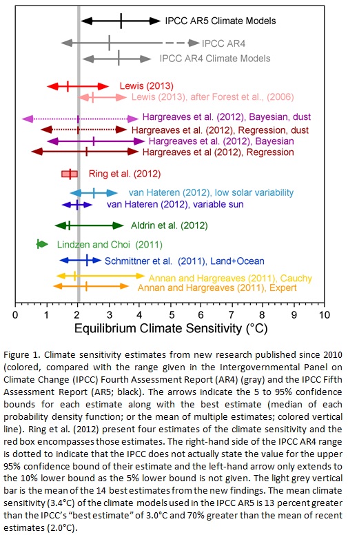
A comparison to various past estimates of ECS is made in figure 5. The base for figure 5 comes from the following weblink :
http://www.cato.org/sites/cato.org/files/wp-content/uploads/gsr_042513_fig1.jpg
See link for the original figure.

Figure 5 : Comparison of the results of this study (1.8) to other recent ECS estimates.
The estimate derived from this study agrees very closely with other recent studies. The gray line on figure 5 at a value of 2.0 represents the mean of 14 recent studies. Looking at the MSE curve in figure 4, 2.0 is essentially flat with 1.8 and would have a similar probability. This study further reinforces the conclusions of other recent studies which suggest climate sensitivity to CO2 is low relative to IPCC estimates .
The big difference with this study is that it is strictly based on the observed data. There are no models involved and only one assumption – that the longer period variation in temperature is driven by CO2 only. Given that the conclusion of a most likely sensitivity of 1.8 ° C / doubling is based on 163 years of observed data, the conclusion is likely to be quite robust.
A brief discussion of the assumption will now be made in light of the conclusion. The question to be asked is : If there are other factors affecting the long period trend of the observed temperature trend (there are many other potential factors, none of which will be discussed in this paper), what does that mean in terms of this best fit ECS curve ?
There are 2 options. If the true ECS is higher than 1.8, by definition , to match the observed data, there has to be some sort of negative forcing in the climate system pushing the temperature down from where it would be expected to be. In this scenario, CO2 forcing would be preventing the temperature trend from falling and is providing a net benefit.
The second option is the true ECS is lower than 1.8. In this scenario, also by definition, there has to be another positive forcing in the climate system pushing the temperature up to match the observed data. In this case CO2 forcing is smaller and poses no concern for detrimental effects.
For both of these options, it is hard to paint a picture where CO2 is going to be significantly detrimental to human welfare. The observed temperature and CO2 data over the last 163 years simply doesn’t allow for it.
Conclusion :
Based on data sets over the last 163 years, a most likely ECS of 1.8 ° C / doubling has been determined. This is a simple calculation based only on data , with no complicated computer models needed.
An ECS value of 1.8 is not consistent with any catastrophic warming estimates but is consistent with skeptical arguments that warming will be mild and non-catastrophic. At the current rate of increase of atmospheric CO2 (about 2.1 ppm/yr), and an ECS of 1.8, we should expect 1.0 ° C of warming by 2100. By comparison, we have experienced 0.86 ° C warming since the start of the HADCRUT4 data set. This warming is similar to what would be expected over the next ~ 100 years and has not been catastrophic by any measure.
For comparison of how unlikely the catastrophic scenario is, the IPCC AR5 estimate of 3.4 has an MSE error nearly as large as assuming that CO2 has zero effect on atmospheric temperature (see fig. 4).
There had been much discussion lately of how the climate models are diverging from the observed record over the last 15 years , due to “the pause”. All sorts of explanations have been posited by those supporting a high ECS value. The most obvious resolution is that the true ECS is lower, such as concluded in this paper. Note how “the pause” brings the observed temperature curve right to the 1.8 ECS synthetic record (see fig. 3). Given an ECS of 1.8, the global temperature is right where one would predict it should be. No convoluted explanations for “the pause” are needed with a lower ECS.
The high sensitivity values used by the IPCC , with their assumption that long term temperature trends are driven by CO2, are completely unsupportable based on the observed data. Along with that, all conclusions of “climate change” catastrophes are also completely unsupportable because they have the high ECS values the IPCC uses built into them (high ECS to get large temperature changes to get catastrophic effects).
Furthermore and most importantly, any policy changes designed to curb “climate change” are also unsupportable based on the data. It is assumed that the need for these policies is because of potential future catastrophic effects of CO2 but that is predicated on the high ECS values of the IPCC.
Files:
I have also attached a spreadsheet with all my raw data and calculations so anyone can easily replicate the work.
ECS Data (xlsx)
=============================================================
About Jeff:
I have followed the climate debate since the 90s. I was an early “skeptic” based on my geologic background – having knowledge of how climate had varied over geologic time, the fact that no one was talking about natural variation and natural cycles was an immediate red flag. The further I dug into the subject, the more I realized there were substantial scientific problems. The paper I am submitting is a paper I have wanted to write for years , as I did the basic calculations several years ago & realized there was no support in the observed data for high climate sensitivity.
ferdberple says:
February 15, 2014 at 7:41 am
“The IPCC says CO2 is responsible for about 1/2 the warming. The author shows 1.8C under the assumption that CO2 is 100% responsible. Which means the author has set an upper limit for TCR below 1.8C*1/2 = 0.9C based on observed data.”
And if the IPCC has got that wrong as well? I pitch it below 0.5C based on the work I have done.
rgbatduke says:
February 14, 2014 at 11:02 am
Perturbed parameter ensemble runs of the various CMIP5 models fairly clearly indicate that the future 100 year integrations of climate are highly “sensitive” to tiny perturbations of the initial conditions
==============
To the extent the models describe the climate system, doesn’t this high sensitivity to initial condition provide some measure of natural variability?
For example, say you had a model that showed 2C variability between runs. Now the IPCC says you can average this out and the average is your forecast. This is statistical nonsense. The future is not an average. It is a probability function, like a throw of the dice.
When you throw the dice, you might get 2, you might get 12. You are most likely to get 7, which is the average, but this doesn’t mean you will get 7. This difference between 2 and 12; 10 gives a measure of the natural variability that can result from a throw of the dice.
So the 2C variability in the model is telling us something useful about the future. That we might see as much as a 2C swing in temperature without any change in forcings. So when we look at the IPCC spaghetti graph, it is showing something very informative that seems to have been largely over looked, perhaps because it runs contrary to the IPCC position of low natural variability.
The IPCC spaghetti graph shows a wide variability between model runs. And this graph is itself is composed of averages, so the raw data must show even more variability. And to the degree that the models describe reality, what the variability in the model runs is showing us is the natural variability that will result without any change in forcings. Thus, the models are showing us that natural variability is high.
ferdberple:
At February 15, 2014 at 9:56 am you conclude
Sorry, but no.
The models only indicate how the models operate. They are not validated as being representative of the climate system.
Hence, the models are only showing us that variability of model behaviour is high.
Richard
RichardLH says
And if the IPCC has got that wrong as well? I pitch it below 0.5C based on the work I have done.
Henry says
I am not sure if you know, but by taking part in photosythesis, carbondioxide extracts energy from the atmosphere, to make greenery and higher carbohydrates and sugars (food).
So, do you have any figures on this (note that the biosphere has been increasing) (e.g. -0.?) and if not, how do you know for sure that the net effect of more CO2 is warming rather than cooling?
Alex Hamilton says:
February 15, 2014 at 4:25 am
John Finn
I have a far better and more accurate understanding of thermodynamics than Dr Roy Spencer.
——————————————————————————————————-
And I have a full understanding of both special and general relativity, including one-paragraph proofs of both which I worked out in some spare time a while back.
Like you, I won’t bother to back that assertion up in any way.
ferdberple says:
“doesn’t that assume the the climate was in equilibrium at the start of the temperature record?
Excellent point! Yes, it does sort of assume that. If we assumed it was equaly distant from equilibrium at the beginning and end (unlikely, but more likely than the condition of closest to equilibrium at the beginning and furthest at the end) then it would be equilibrium sensitivity.
So, we can say with even greater confidence that given the data CO2 isn’t a problem.
HenryP says:
February 15, 2014 at 10:13 am
“So, do you have any figures on this (note that the biosphere has been increasing) (e.g. -0.?) and if not, how do you know for sure that the net effect of more CO2 is warming rather than cooling?”
Observation and logic has it that the system remains within an overall stability despite other factors coming that could possibly deflect it.
This would appear to be a sign that there are many, opportunistic, feed back loops that keep the overall picture stable.
How much any individual, tiny, details matter is a great puzzle.
richardscourtney says:
February 15, 2014 at 10:07 am
“Hence, the models are only showing us that variability of model behaviour is high.”
and the probably that “The Wisdom of Crowds” can apply equally to deluded idiots as well as ordinary people. The challenge is in finding which group it is that you are studying.
RichardLH:
At February 15, 2014 at 11:47 am you write
I said nothing about “idiots”, “ordinary people” or any “group” of such.
I was commenting on climate models.
Richard
RichardLH says
How much any individual, tiny, details matter is a great puzzle.
Henry says
The problem is that you claim to know that it lies between 0 and 0.5
(we are talking of a difference of 0.01% in the composition of the atmosphere over 100 years)
Taking also radiative cooling into account, what if it is negative?
Betterfor you is to say that you don’t know if it has any influnce at all (on warming)
http://wattsupwiththat.com/2014/02/13/assessment-of-equilibrium-climate-sensitivity-and-catastrophic-global-warming-potential-based-on-the-historical-data-record/#comment-1567510
and start at the beginning
http://blogs.24.com/henryp/2011/08/11/the-greenhouse-effect-and-the-principle-of-re-radiation-11-aug-2011/
This simple and elegant analysis, based on the data (as good or as bad as it is) it is showing that even assuming that CO_2 would be the only knob affecting the temperature there is no reason for alarmism.
Even if the data sets would be right, with all those adjustments always cooling the past and warming the recent temperatures,
http://stevengoddard.wordpress.com/2014/02/13/a-closer-look-at-ushcn-tobs-adjustments/
http://wattsupwiththat.com/2013/07/15/central-park-in-ushcnv2-5-october-2012-magically-becomes-cooler-in-july-in-the-dust-bowl-years/
ignoring the UHI, assuming everything was caused by anthropogenic CO_2, even in such case, there is no reason for panic.
The only certified effect of the added CO_2 in the atmosphere so far is the increase in the biosphere.
http://www.co2science.org/data/plant_growth/plantgrowth.php
So enjoying the further beneficial CO_2 effect, we can concentrate on improving human life and ignore the prophets of doom.
Thank you for this Jeff L., I almost can hear the relief in the very stressed warmist camp, come on boys and girls, we will be ok stop doing this to you:
http://notrickszone.com/2013/10/31/green-psychologists-confirm-climate-alarmists-are-making-themselves-mentally-sick-doomer-depression/
richardscourtney says:
February 15, 2014 at 11:57 am
“I said nothing about “idiots”, “ordinary people” or any “group” of such.
I was commenting on climate models.”
Allegory.
I was observing that “The Wisdom of Crowds” which applies to the statistics assessing questions posed to a group of people of unknown origin as well as a well selected group by using an average to deduce an accurate result from a group of widely disparate choices has also been used to derive a conclusion from Climate Models.
It was a wry observation that an average so produced may well be wrong as well as right.
HenryP says:
February 15, 2014 at 12:01 pm
“The problem is that you claim to know that it lies between 0 and 0.5”
Please do not re-phrase what I said.
I said the data indicates that it lies between 0 and 0.5 assuming a reasonable distribution into the other factors that have to be taken into account.
I’m starting to see a series of instant replays of the typical arguments – in particular those involving the Dean of “Science is Settled U.” – James Hansen. Without casting any aspersions on the AGWer’s can anyone who is happy to quote politically loaded pronouncements from James Hansen — quote anything which Dr. Hansen has written and which has been found to be scientifically reliable and valid when tested — I presume that he published a dissertation — has anyone ever read it?
To put this discussion in simple terms ==> You Can’t !!
1) To try to unravel the onion — let’s see if there are things which we can agree on:
a. The earth-sun system is fiendishly complex. Nevertheless, It is relatively easy to make reasonably well characterized measurements which are local in-time and space of various parameters — such as the current temperature of the air at human height near to my house in a suburb of Boston. I have up to 6 wired, wireless and the old fashioned optically monitored thermometers located at various heights, distances from the structure, cardinal directions, amounts of shade, etc.. To a general level they agree with interesting variability depending on the seasons, time of day, weather, etc.
b. However, Its considerably more difficult to develop a well characterized spatially averaged value for a given parameter
c. and even more difficult to develop meaningful time series of these global values.
Why — because things change beyond our control such as the immediate surroundings of a monitoring station; instrumentation used; or the protocols used to make the measurements and calibrate.. Corrections can be applied to the individual datums or various aggregates — but they can never be verified without access to the Proverbial Time Machine. So what we have to work with is poorly characterized time series of data which we even less reliably attempt to average.
2) From now on I’m assuming that some of us will not agree with the following:
a. Now to try to characterize the behavior of one such difficult to quantify parameter — e.g. the earth’s surface temperature measurements in terms of any one other parameter, e.g. global CO2 conentration in the atmosphere is a fools errand
b. The vaunted models are even worse as we don’t know which elements of the overall physics has been omitted from the model let alone the relevant weighting factor to apply to each scalar or vector parameter —
c. The above results in the despicable practice of fitting the model with an abundance of guestimated weighting factors which seem to change as needed to meet the political requirements.
3) Hope now that most will be tuned back in a agree with the following:
a. The only thing that we can say with reasonable certainty is that whatever we [people the rest of the biosphere and even the geology] do here will have no noticeable impact on the behavior of the sun.
b. Almost nothing can be categorically excluded with respect to the influence of the Sun on the behavior of the overall system.
4) To then use the results of these hopelessly incompletely constructed models as the basis for public policy which has the potential to disadvantage millions and possibly destroy the most productive global economy in history is far beyond insanity — its criminal insanity.
5) Instead of wasting Billions on Solyndria, Ivanophahotep? and CapeWind – here’s a policy every country on the planet can contribute to in a meaningful way:
a. Fund as yet uncorrupted students to:
i. Design good, long MTBF easily, fabricated, easily deployed and maintained automated instrumentation with cloud-based global access to the raw data
ii. Design web-based experimental protocols and data analysis tools — as if we were planning a Voyager-type mission to planet earth – 15 years should suffice
b. “Launch” and collect good data for the next 50+ years
c. Fund students to challenge the accepted and orthodox interpretation of the real-time data and any paleo, proxy, etc.
d. Somewhere around 2080 we can revisit the question of APG or not and if so how much.
e. Meantime we can always build a few seawalls to adapt to the changes as we always have adapted to a changing climate in the past.
richardscourtney says:
February 15, 2014 at 10:07 am
They are not validated as being representative of the climate system.
============
I agree. My argument is that the IPCC believes the models are representative. If you accept this belief as correct, then the models are telling us that natural variability is high.
The IPCC argument in support of CO2 warming is largely based on the position that natural variability is low, and could not have caused the late 20th century warming. But the models themselves are saying that variability is high, which is consistent with the “pause”.
”
Alex Hamilton says:
February 15, 2014 at 2:37 am
Monckton of Brenchley
I refer to your comment pertaining to climate sensitivity and I am of course aware of your efforts in the field. I respect your knowledge of the history of all this, but, when it comes to science,the only thing I respect is the truth based on valid science and empirical data.
There is a whole new paradigm emerging, Sir, which I believe you need to heed and which I have outlined in my comments on this thread. The greenhouse radiative forcing conjecture can be shown to be incorrect with valid physics. There is no “33 degrees of warrming” supposedly caused by back radiation from the cold atmosphere. Radiation doesn’t raise the temperature of a warmer body. Thus you cannot calculate sensitivity to radiating gases because the underlying assumption is false.
”
Sorry alex but your paradigm results in the conclusion that wearing a coat doesn’t help when you’re out in the cold. There’s so much energy coming to the Earth’s surface, mostly from the Sun, a little from the planet’s interior and a pittance from man using energy. To quantify, we get an average power input of around 240 W/m^2. We enjoy a global average temperature of around 288 kelvins. The surface radiates about 390 W/m^2 on average. Notice that we do not have enough incoming power (240 W/m^2) to compensate for the 390 W/m^2 power radiated. There’s about 150 W/m^2 discrepancy here – enough to cause the Earth to cool off by about33 deg C before the outgoing power is balanced again by the incoming.
When it comes to matter, everything above absolute zero is going to radiate power. When something is the same temperature as its surroundings, it will still continue to radiate the same amount of power – based upon its own temperature. This object will stay at the same temperature as its surroundings and that means also that there can be no net flow of energy into or out of the object. It it were not this way, then an object that behaves this way could be placed into a box of the same temperature and this object would change temperature away from its original temperature. If you can come up with this, you’ve just solved the energy problem of mankind forever because you have just invented the perpetual motion heat engine – no additional energy sources needed. Better go secure your patent before the Japanese figure it out and beat you to it.
WestHighlander says:
February 15, 2014 at 1:47 pm
Actually I can sum it up in two words. (for the measurements anyway)
Nyquist Rate.
If you wish to accurately determine a field and its evolution in time then you need to sample at better than twice the expected maximum spacial trend curve (2D grid if at a fixed potion above the ground – say 2 meters) and better that twice the expected maximum rate of change – preferably below hourly at the very least in this case.
Now if we had that number of continuously recording thermometers…..
Otherwise it is just a glorified guess/estimate with error bounds you could drive all sorts of things through.
Shame on all of you from both sides of the AGW issue who are so critical of Jeff L’s reasoning and work. Especially you Willis E. who I somewhat admired before your rants in your comments here to Jeff L. He made it clear he was looking to bound the possible effects of CO2 and he did.
The important lags you are harping on are incorporated into the HadCRUT data for CO2 rise in previous years…..and read on before you reply. I endorse the supportive comments from Jim Cripwell and Doc Martyn.
And to all of you who beat up on Jeff about ECS, if he didn’t understand completely the differences between ECS and TCR, then he had the same problem I did until about 9 months ago, because it isn’t talked about that much in the peer-reviewed literature. You want proof? Ask yourself why our EPA is focused on ECS and not TCR in trying to predict global warming over the next couple of centuries, while writing their CO2 emissions control regulations focused on that period of time. ECS is a purely academic concept that can’t be verified by actual physical data. The IPCC’s other climate sensitivity metric, TCR, also theoretically can’t be verified by physical data. What climate sensitivity metric does the IPCC utilize that could actually be verified by actual physical data? That they don’t demonstrates their ill-advised dependence on un-validated climate models. Focusing on ECS that is such the impractical darling of peer-reviewed research, is a waste of resources for many reasons too numerous to list here, if one is really trying to understand what will happen with AGW over the next couple of centuries. The ECS forcing scenario is preposterous, unrealistic and a total waste of computer time.
Jeff L has extracted from the HadCRUT4 data an upper bound for what I define as Total Radiative Force (TRF) Transient Climate Sensitivity (TCS). That is the global average surface temperature achieved in the year CO2 doubles in the atmosphere from the actual slowly rising TRF. The TRF involved is from CO2, other GHG, and primarily Total Solar Irradiance (TSI) changes referenced to 1850 levels. Natural climate cycles in play can skew the results either way. If the internal dynamics of the climate system provides surface warming over the data analysis period, then Jeff L’s approach is conservative in identifying TCS TCR. If there is something cooling it (and there is very some slow cooling from the Milankovic’ cycle) then his analysis may underestimate climate sensitivity to CO2, but we can bound that possibility also in trying to figure out how much AGW we can possibly get before we run out of all fossil fuels on the planet to burn within 125 years. One has to be aware of the approx. 60 year internal climate cycles and what effect they may have on Jeff’s straightforward analysis method. If you pick a time period that goes from one peak in this cycle to a peak several cycles later then you can minimize the effects of this natural climate cycle on the accuracy of his analysis method.
For all of you who beat Jeff up about equilibrium conditions, I submit that the climate is approximately in equilibrium for the average total radiative force in any year, if the radiative forcing applied is very gradually like it actually is in the real world. Don’t believe me? Consider a simple spring-mass-damper system in a 1G gravity field and that initially you are holding the mass in place by pushing upward on the mass with a constant force = 1/4 the tension force in the spring and the mass is at rest. If you slowly start to increase the upward force by pushing up with your finger to a new equilibrium position such that the final increased force you apply to the mass is twice the initial force (equal to 1/2 the original tension force in the spring) and then you stop pushing and hold the mass in place with this final force, the mass is in a new equilibrium position with twice the initial upward force and you just hold it there. If you take care to push the mass very slowly upward so you don’t excite any oscillatory behavior, the mass undergoes a gradually changing equilibrium condition that can be assumed to be constant in any one year. So when the CO2 reaches a doubled value in the atmosphere, because of non-linearities in the climate system, some CO2 transfers to the atmosphere from warming oceans and land masses, but when the CO2 in the atmosphere reaches a doubled value, some injected and some from the earth’s surface, the climate will be in a new quasi-steady equilibrium point for that Total Radiative Force level.
Once an upper bound for the TRF TCS value is extracted from the data using Jeff’ approach, it can be corrected for any TSI changes that occurred over the data analysis period. When considering the actual slow gradual radiative force rise when CO2 and TSI are both increasing over a long period of time, thinking about the simple dynamics problem above will lead you to understand that TCS as defined here, is approximately equal to TCR. The average of TCR and ECS values in Table 8.2 of the IPCC AR4 report provide an average ratio of ECS/TCR = 1.8. Therefore, if TCS = TCR, then ECS = (Jeff L’s 1.8 deg C value)(1.8) = 3.2 deg C. However, Jeff L’s 1.8 deg C value extracted from the data can be lowered to 1.6 deg C by correcting for about 0.4 W/m^2 TSI rise from 1850 to 2010. Also his sensitivity value is for all GHG effects since 1850, not just CO2, but germane to bounding the AGW threat Throwing out some spurious “out of family” HadCrut4 data points like the 1998 data point we know is associated with a naturally occurring El Nino event that yea,r could get his upper bound value a little lower to my least upper bound value for ECS = 2.5 deg C. But, he has performed a very simple and easy to understand analysis that is much, much better than the IPCC AR5 report’s new climate sensitivity uncertainty range of 1.5 < ECS < 4.5 deg C. And he did it simply and inexpensively.
All of you take notice because more of us are going to join his bandwagon to rigorously lower the IPCC ECS uncertainty range using similar reasoning. The upper bound for ECS buried in the HadCRUT4 data is below the mid-point of the official IPCC uncertainty range. But we shouldn't be bothering with ECS to predict climate over the next 200 years. TCS as extracted from the data, is a more appropriate measure of climate sensitivity we really need to be worried about. If you use methods similar to Jeff's to bound all-GHG TCS and consider the remaining economically recoverable fossil fuels on the planet, we can only get about 1 deg C more of AGW warming before we have to be completely transitioned to alternative fuels that do not emit CO2.
To other critics that pointed out the hadCRUT4 Global Average Temperature Anomaly (GATA) is not global average surface temperature (GAST), what else are you going to use to cut through all the BS from the IPCC and get them to get real about a useful climate sensitivity metric that could be used to accurately assess the maximum possible "heat pulse" we might get from AGW over the next 200 years? Its time to cut off all of the alarm bells, agree that climate sensitivity of importance is not ECS and closer to TCS = TCR and work the problem.
The peer-reviewed literature on climate science is voluminous and full of useless claims. Amateurs like Jeff and myself don't have time to wade through all of this mostly useless literature. What reputable journal would even publish results of a study based only on results of un-validated climate models. Those of us who have to solve critical problems quickly in the real world can do something simple to try to bound the problem and Jeff L. did. Please congratulate him for his interesting effort and help him to get closer to the truth. Don't bully and discourage him with your nasty and pompous remarks.
@Dale Rainwater Burns, rgbatduke –
I think your comments cut to the real issues – both the lag of CO2 to temperature, and the range of natural variation, which together blow ANY definitive claims of significant warming effect from CO2, let alone from human emission of CO2 (and let’s don’t forget that human BREATHING emits a major fraction of what burning coal does! and animal respiration many times more) out of the water. If you consider the entire historical record and paleo record, the lack of correlation between CO2 concentrations and temps is incontrovertible.
If you are going to plot climate response to influencing factors realistically, you have to consider a lot more than CO2, which is actually minuscule compared to the Sun, the Earth’s orbital motions and the behavior of ocean currents. It’s actually a very minor factor in the overall climate picture, demonstrably much less even than the variation or noise in the actual major drivers of climate. If you don’t do it that way, you repeat the error of alarmists who fixate on CO2.
Harold H Doiron, PhD says:
February 15, 2014 at 6:29 pm
Oh, please, stop your pearl-clutching. Many people pointed out mistakes Jeff made, myself included. Because of the mistakes he made, he didn’t even come close to being able to “bound the possible effects of CO2”.
If he listens to the scientific objections various people made to his work, he could actually get much closer to what he’s trying to do. For example, I said:
If he does that, his understanding will be greater and his future work will be stronger … what’s not to like?
On the other hand, if he listens to you whine and bitch about all the mean, krool people like myself who pointed out his mistakes, he’ll never get anywhere.
Science is a blood sport, Harold. You put your ideas out there, hand around the hammers, and invite people to see if they can break it. You don’t bitch when they do just that, you invite them to do just that.
You don’t complain about peoples’ objections. You learn from them. That’s science.
w.
PS—I am as even-handed as I can be, in that I make every effort to apply the same standards to skeptics as to activists. I’m sorry if that offends you, but bad science is bad science on either side of the aisle.
I do love it, however, when folks agree with my standards when I apply them to activists, but suddenly I’m an idiot and a bad person when I apply them to skeptics …
RichardLH says
http://wattsupwiththat.com/2014/02/13/assessment-of-equilibrium-climate-sensitivity-and-catastrophic-global-warming-potential-based-on-the-historical-data-record/#comment-1568811
Henry says
you were challenged to bring a balance sheet showing me how much cooling and how much warming is caused by an increase of 0.01% of CO2.
If you cannot bring any proof, how can you make any claim that it must have some warming effect?
I, OTOH, showed you that minimum temps. have been falling faster than means and therefore the CO2 warming mantra is false and utter scientific nonsense.
There is no global warming and there is no man made global warming. There has not been global warming for a long time, period. My results clearly showed that there is only global cooling,
http://www.woodfortrees.org/plot/hadcrut4gl/from:1987/to:2015/plot/hadcrut4gl/from:2002/to:2015/trend/plot/hadcrut3gl/from:1987/to:2015/plot/hadcrut3gl/from:2002/to:2015/trend/plot/rss/from:1987/to:2015/plot/rss/from:2002/to:2015/trend/plot/hadsst2gl/from:1987/to:2015/plot/hadsst2gl/from:2002/to:2015/trend/plot/hadcrut4gl/from:1987/to:2002/trend/plot/hadcrut3gl/from:1987/to:2002/trend/plot/hadsst2gl/from:1987/to:2002/trend/plot/rss/from:1987/to:2002/trend
and this this will go for the next 2-3 decades.
Note that there are going to be a few problems due to this global cooling
e.g. the jets stay further south, flooding England
At the higher latitudes >[40] it will become progressively drier, from now onward, ultimately culminating in a big drought period similar to the dust bowl drought 1932-1939. My various calculations all bring me to believe that this main drought period on the Great Plains will be from 2021-2028. It looks like we have only 7 “fat” years left…..
The sooner we get everybody off their CO2 warmed horsebacks , the better we can plan for the bleak future coming up ahead.
Willis Eschenbach says:
February 16, 2014 at 12:03 am
Oh, please, stop your pearl-clutching. Many people pointed out mistakes Jeff made, myself included. Because of the mistakes he made, he didn’t even come close to being able to “bound the possible effects of CO2″.
[…]
——————————————————————————————————————–
Willis, while your suggestion for testing the OP out of sample has a lot of merit, I can’t help feeling that you’re falling nto the same mistake as others of reading more into the post than was ever intended. That’s maybe not surprising seeing as most people on both sides of the climate debate seem to be forever looking for a “smoking gun” or silver bullet. But that’s not what the Op was ever offering.
Let’s say I want to get a feel for the Sun’s energy output.
I could set out a few solar panels in my back yard in the UK and measure the energy they capture. I find that I capture about 125 W / m^2. From that it would be madness to back-calcuate and claim I had an accurate figure for the Great Fireball’s output but I would be perfectly entitled to calculate back and say something like:
“Assuming the solar energy per area falling on the uk equals the average energy falling across the Earth’s surface, the total output of the Sun is at least the value I’ve calculated.
That statement takes no account of factors such as the efficiency of my panels, their response to different wavelengths, the atmosphere or anything else intercepting the incoming radiation but it would still be valid statement if I took my measurements using a selenium cell under cloudy skies during a total eclipse!
The complaints about TCS / ECS are more or less irrelevant because (a) the climate is never in equilibrium and (b) they’re both defined in terms of an instantaneous doubling of CO2 which is a physical absurdity. Unless the lag to ECS is several centuries the actual rate of increase is slow enough for thde climate to keep up.
The complaints about factors he’s ignored are irrelevant because (a) he’s openly stated that he’s ignored them, (b) they will ALL tend to reduce, rather than increase, the observed direct response to CO2 under the “CO2 does it all” assumption, so they will ALL lead to a lower figure in reality and (c) he’s (briefly) considered what the implications of including any other factors would be, regardless of the “direction” in which they operate.
Incidentally, that final point is where your suggestion of looking out of sample falters a little. It would be an interesting exercise in its own right but unless the assumption that “it’s all CO2” is actually true we would expect a model that ignores lots of known factors to fail out of sample. If it didn’t then it would be telling us that it really IS “all CO2”, which would be an incredible result
You’re quite right that science progresses by inviting people to knock holes in your ideas, but that’s only true when the people with the hammers actually aim at your ideas, rather than what they imagine your ideas to be!
wbrozek says:
Are you sure this is the right way around? See the following where lower temperatures occurred after CO2 reached its peak.
http://motls.blogspot.ca/2006/07/carbon-dioxide-and-temperatures-ice.html
-yes, I know it is a common misunderstanding that some people have that climate scientists assert that CO2 changes caused the milankovitch cycles (ice age cycles). What climate scientists actually say is that the CO2 changes respond to the changes in the temperatures caused by the solar cycle, that the changes in CO2 produces a positive feedback (CO2 goes down when temps go down slightly, water vapor goes down even more, then temperatures go down even further). . . and vice versa during a warming period, warming causes more CO2 due to carbon cycle feedbacks, more warming ensues producing more water vapor, etc.
The climate scientists know that this is true because they can precisely measure the difference in the amount of heat energy produced by the solar cycles and the understand that it simply isn’t enough by itself to cause the changes in temperature that have been observed.
Alex Hamilton says:
“I have a far better and more accurate understanding of thermodynamics than Dr Roy Spencer.”
I think not.
+++++++++++++++++++
jai mitchell says:
“…the amount of heat energy produced by the solar cycles and the understand that it simply isn’t enough by itself to cause the changes in temperature that have been observed.”
The implication is that CO2 is the culprit. How do I know this? I know, because it is jai mitchell’s comment. ☺
But as Pat Frank notes above, there is still zero hard evidence that any of the warming since 1880 is due to increased atmospheric CO2.
Almost all of the effect from CO2 happened in the first few dozen parts per million of atmospheric concentration. Since then, all added CO2 has been, in effect, ‘painting the window’ again. The first coat of paint had by far the greatest effect. But now, the effect of any additional CO2 is so small that it is not even measurable.
There is no catastrophic global warming. There isn’t even any hint of such. All of the many alarmist predictions of catastrophic AGW have come to nothing. The only remaining question is: why would jai mitchell or anyone else still believe in that debunked nonsense?
One additional comment:
jai mitchell says is that: “…CO2 changes respond to the changes in the temperatures…”
If mitchell stops there, we are in agreement. Because there is verifiable, measurable scientific evidence showing that comment is correct [while there are no verifiable, testable measurements showing that ∆CO2 causes ∆T].
Beyond stating that ∆T causes ∆CO2, there is no measurable, testable evidence that the rest is so. It is merely an assertion; a conjecture. An opinion.
Baseless assertions are good enough at SkS, tamino, realclimate, etc. But they aren’t good enough here at the internet’s “Best Science & Technology” site. Here, we need verifiable measurements.