This exercise in data analysis pins down a value of 1.8C for ECS.
Guest essay by Jeff L.
Introduction:
If the global climate debate between skeptics and alarmists were cooked down to one topic, it would be Equilibrium Climate Sensitivity to CO2 (ECS) , or how much will the atmosphere warm for a given increase in CO2 .
Temperature change as a function of CO2 concentration is a logarithmic function, so ECS is commonly expressed as X ° C per doubling of CO2. Estimates vary widely , from less than 1 ° C/ doubling to over 5 ° C / doubling. Alarmists would suggest sensitivity is on the high end and that catastrophic effects are inevitable. Skeptics would say sensitivity is on the low end and any changes will be non-catastrophic and easily adapted to.
All potential “catastrophic” consequences are based on one key assumption : High ECS ( generally > 3.0 ° C/ doubling of CO2). Without high sensitivity , there will not be large temperature changes and there will not be catastrophic consequences. As such, this is essentially the crux of the argument : if sensitivity is not high, all the “catastrophic” and destructive effects hypothesized will not happen. One could argue this makes ECS the most fundamental quantity to be understood.
In general, those who are supportive of the catastrophic hypothesis reach their conclusion based on global climate model output. As has been observed by many interested in the climate debate, over the last 15 + years, there has been a “pause” in global warming, illustrating that there are significant uncertainties in the validity of global climate models and the ECS associated with them.
There is a better alternative to using models to test the hypothesis of high ECS. We have temperature and CO2 data from pre-industrial times to present day. According to the catastrophic theory, the driver of all longer trends in modern temperature changes is CO2. As such, the catastrophic hypothesis is easily tested with the available data. We can use the CO2 record to calculate a series of synthetic temperature records using different assumed sensitivities and see what sensitivity best matches the observed temperature record.
The rest of this paper will explore testing the hypothesis of high ECS based on the observed data. I want to re-iterate the assumption of this hypothesis, which is also the assumption of the catastrophists position, that all longer term temperature change is driven by changes in CO2. I do not want to imply that I necessarily endorse this assumption, but I do want to illustrate the implications of this assumption. This is important to keep in mind as I will attribute all longer term temperature changes to CO2 in this analysis. I will comment at the end of this paper on the implications if this assumption is violated.
Data:
There are several potential datasets that could be used for the global temperature record. One of the longer and more commonly referenced datasets is HADCRUT4, which I have used for this study (plotted in fig. 1) The data may be found at the following weblink :
http://www.cru.uea.ac.uk/cru/data/temperature/HadCRUT4-gl.dat
I have used the annualized Global Average Annual Temperature anomaly from this data set. This data record starts in 1850 and goes to present, so we have 163 years of data. For the purposes on this analysis, the various adjustments that have been made to the data over the years will make very little difference to the best fit ECS. I will calculate what ECS best fits this temperature record, given the CO2 record.

Figure 1 : HADCRUT4 Global Average Annual Temperature Anomaly
The CO2 data set is from 2 sources. From 1959 to present, the Mauna Loa annual mean CO2 concentration is used. The data may be found at the following weblink :
ftp://aftp.cmdl.noaa.gov/products/trends/co2/co2_annmean_mlo.txt
For pre-1959, ice core data from Law Dome is used. The data may be found at the following weblink :
ftp://ftp.ncdc.noaa.gov/pub/data/paleo/icecore/antarctica/law/law_co2.txt
The Law Dome data record runs from 1832 to 1978. This is important for 2 reasons. First, and most importantly, it overlaps Mauna Loa data set. It can easily be seen in figure 2 that it is internally consistent with the Mauna Loa data set, thus providing higher confidence in the pre-Mauna Loa portion of the record. Second, the start of the data record pre-dates the start of the HADCRUT4 temperature record, allowing estimates of ECS to be tested against the entire HADCRUT4 temperature record. For the calculations that follow, a simple splice of the pre-1959 Law Dome data onto the Mauna Loa data was made , as the two data sets tie with little offset.

Figure 2 : Modern CO2 concentration record from Mauna Loa and Law Dome Ice Core.
Calculations:
From the above CO2 record, a set of synthetic temperature records can be constructed with various assumed ECS values. The synthetic records can then be compared to the observed data (HADCRUT4) and a determination of the best fit ECS can be made.
The equation needed for the calculation of the synthetic temperature record is as follows :
∆T = ECS* ln(C2/C1)) / ln(2)
where :
∆T = Change in temperature, ° C
ECS = Equilibrium Climate Sensitivity , ° C /doubling
C1 = CO2 concentration (PPM) at time 1
C2 = CO2 concentration (PPM) at time 2
For the purposes of this test of sensitivity, I set time 1 to 1850, the start of the HADCRUT4 temperature dataset. C1 at the same time from the Law Dome data set is 284.7 PPM. For each year from 1850 to 2013, I use the appropriate C2 value for that time and calculate ∆T with the formula above. To tie back to the HADCRUT4 data set, I use the HADCRUT4 temperature anomaly in 1850 ( -0.374 ° C) and add on the calculated ∆T value to create a synthetic temperature record.
ECS values ranging from 0.0 to 5.0 ° C /doubling were used to create a series of synthetic temperature records. Figure 3 shows the calculated synthetic records, labeled by their input ECS, as well as the observed HADCRUT4 data.

Figure 3: HADCRUT4 Observed data and synthetic temperature records for ECS values between 0.0 and 5.0 ° C / doubling. Where not labeled, synthetic records are at increments of 0.2 ° C / doubling. Warmer colors are warmer synthetic records.
From Figure 3, it is visually apparent that a ECS value somewhere close to 2.0 ° C/ doubling is a reasonable match to the observed data. This can be more specifically quantified by calculating the Mean Squared Error (MSE) of the synthetic records against the observed data. This is a “goodness of fit” measurement, with the minimum MSE representing the best fit ECS value. Figure 4 is a plot of MSE values for each ECS synthetic record.

Figure 4 : Mean Squared Error vs ECS values. A few ECS values of interest are labeled for further discussion
In plotting, the MSE values, a ECS value 1.8 ° C/ doubling is found to have the minimum MSE and thus is determined to be the best estimate of ECS based on the observed data over the last 163 years.
Discussion :
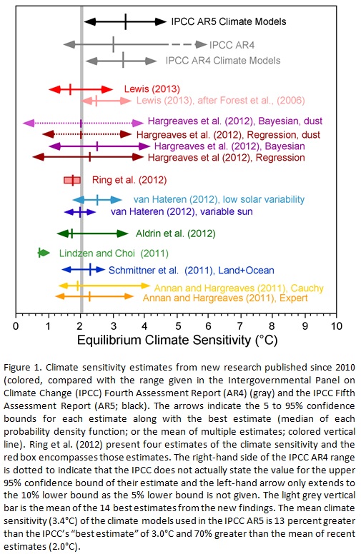
A comparison to various past estimates of ECS is made in figure 5. The base for figure 5 comes from the following weblink :
http://www.cato.org/sites/cato.org/files/wp-content/uploads/gsr_042513_fig1.jpg
See link for the original figure.

Figure 5 : Comparison of the results of this study (1.8) to other recent ECS estimates.
The estimate derived from this study agrees very closely with other recent studies. The gray line on figure 5 at a value of 2.0 represents the mean of 14 recent studies. Looking at the MSE curve in figure 4, 2.0 is essentially flat with 1.8 and would have a similar probability. This study further reinforces the conclusions of other recent studies which suggest climate sensitivity to CO2 is low relative to IPCC estimates .
The big difference with this study is that it is strictly based on the observed data. There are no models involved and only one assumption – that the longer period variation in temperature is driven by CO2 only. Given that the conclusion of a most likely sensitivity of 1.8 ° C / doubling is based on 163 years of observed data, the conclusion is likely to be quite robust.
A brief discussion of the assumption will now be made in light of the conclusion. The question to be asked is : If there are other factors affecting the long period trend of the observed temperature trend (there are many other potential factors, none of which will be discussed in this paper), what does that mean in terms of this best fit ECS curve ?
There are 2 options. If the true ECS is higher than 1.8, by definition , to match the observed data, there has to be some sort of negative forcing in the climate system pushing the temperature down from where it would be expected to be. In this scenario, CO2 forcing would be preventing the temperature trend from falling and is providing a net benefit.
The second option is the true ECS is lower than 1.8. In this scenario, also by definition, there has to be another positive forcing in the climate system pushing the temperature up to match the observed data. In this case CO2 forcing is smaller and poses no concern for detrimental effects.
For both of these options, it is hard to paint a picture where CO2 is going to be significantly detrimental to human welfare. The observed temperature and CO2 data over the last 163 years simply doesn’t allow for it.
Conclusion :
Based on data sets over the last 163 years, a most likely ECS of 1.8 ° C / doubling has been determined. This is a simple calculation based only on data , with no complicated computer models needed.
An ECS value of 1.8 is not consistent with any catastrophic warming estimates but is consistent with skeptical arguments that warming will be mild and non-catastrophic. At the current rate of increase of atmospheric CO2 (about 2.1 ppm/yr), and an ECS of 1.8, we should expect 1.0 ° C of warming by 2100. By comparison, we have experienced 0.86 ° C warming since the start of the HADCRUT4 data set. This warming is similar to what would be expected over the next ~ 100 years and has not been catastrophic by any measure.
For comparison of how unlikely the catastrophic scenario is, the IPCC AR5 estimate of 3.4 has an MSE error nearly as large as assuming that CO2 has zero effect on atmospheric temperature (see fig. 4).
There had been much discussion lately of how the climate models are diverging from the observed record over the last 15 years , due to “the pause”. All sorts of explanations have been posited by those supporting a high ECS value. The most obvious resolution is that the true ECS is lower, such as concluded in this paper. Note how “the pause” brings the observed temperature curve right to the 1.8 ECS synthetic record (see fig. 3). Given an ECS of 1.8, the global temperature is right where one would predict it should be. No convoluted explanations for “the pause” are needed with a lower ECS.
The high sensitivity values used by the IPCC , with their assumption that long term temperature trends are driven by CO2, are completely unsupportable based on the observed data. Along with that, all conclusions of “climate change” catastrophes are also completely unsupportable because they have the high ECS values the IPCC uses built into them (high ECS to get large temperature changes to get catastrophic effects).
Furthermore and most importantly, any policy changes designed to curb “climate change” are also unsupportable based on the data. It is assumed that the need for these policies is because of potential future catastrophic effects of CO2 but that is predicated on the high ECS values of the IPCC.
Files:
I have also attached a spreadsheet with all my raw data and calculations so anyone can easily replicate the work.
ECS Data (xlsx)
=============================================================
About Jeff:
I have followed the climate debate since the 90s. I was an early “skeptic” based on my geologic background – having knowledge of how climate had varied over geologic time, the fact that no one was talking about natural variation and natural cycles was an immediate red flag. The further I dug into the subject, the more I realized there were substantial scientific problems. The paper I am submitting is a paper I have wanted to write for years , as I did the basic calculations several years ago & realized there was no support in the observed data for high climate sensitivity.
Alex Hamilton, I agree with you. The whole AGW/GHE thing is not even wrong.
HenryP says:
February 14, 2014 at 12:22 pm
“I know what will happen next: global cooling until around 2040…I don’t think I can give you more clues.”
I do understand that you genuinely believe that you know what will happen next. I too am fairly sure that the immediate trend will be downwards. What I do not know for sure is the depth and length of that period.
The data (and reasonable projections based on that data) do not allow for me to come to a firmer conclusion. IMHO.
Sorry, I am going to sleep now,
I will check you guys tomorrow again
just try to understand me
I even do give an accurate prediction by how much the global temperature will fall
http://blogs.24.com/henryp/2013/04/29/the-climate-is-changing/
it is really fairly simple
by 2040 the temp. will be as it was in 1950.
Don’t confuse energy out with energy in
Good night you all
Jeff L – Although you do comment about your assumption that CO2 is the only significant variable in the temperature rise across the dataset, that still is a classic example of omitted-variable bias.
To start, if you were to include the effect of the ~60 year cycle, you would note it would be near bottom in 1850, 1910, 1970 and top roughly in 1880, 1940 and 2000. The peak to trough swing is about 0.3 C. Because your calculation starts at the bottom of a trough and finishes at the top of a later cycle the swing is overegging the ECS calc. If you remove the 0.3 C as an artefact, it drops your ECS calc to 1.1 C/doubling. It may be less than the full 0.3 C, but it is still highly significant.
The IPCC ensemble modellers are doing exactly the same thing, but are starting one cycle later. Their century is 1906-2005, with the ~60 year cycle being at bottom in 1906.
Including a solar effect would probably also drop the ECS a bit more, but I suspect not much, since 1850 was near solar max of SC9. On the data it looks like 1850 may have been similar to 2005 in combined solar effect. On the other hand there are several papers around finding that solar activity was at a multimillenial peak in 2005 or so.
The third omitted variable is UHIE, which appears to be worth about 0.4 out of the remaining 1.1 C/doubling. That is based on a cross comparison of HadCET and HadCRUT using the same methodology. This is not a perfect like with like comparison, but gives an idea of how much residual UHIE contamination may remain in the HadCRUT dataset. My estimate based on 250 years of HadCET is an ECS of about 0.7 C/doubling with solar (based on BJ1996) and the ~60 year cycle included, but with volcanoes and UHIE excluded.
So, yes, the method may be reasonable, but unless all the significant variables are included you are quite massively overestimating ECS – exactly as the IPCC ensemble modellers are doing.
george e. smith says:
February 14, 2014 at 12:45 pm
George!
I am disappointed in your multiple poor assumptions of:
A perfectly clear sky (seriously -> NO attenuation in the world’s “clear-sky” atmosphere?)
At noon, on the equator on the equinox, is not every other hour of the day at the the rest of the latitudes on the rest of the days of the year.
You used NASA’s “joke” of a yearly average TSI rather than the daily TOA values.
No declination corrction for axial polar tilt for other days of the year.
Regardless, on your “perfectly clear day” on the equinox on the equator, here is the rest of the world’s latitudes. Attenuation factor = 0.85 – adequate for a very clear low humidity polar sky with no clouds, air masses from NOAA and Bason.
Day-of-Year=> 267 1361 <=TSI-this-Year (Average Radiation) Today=> 23-Sep 1353 <=TOA Today (Actual Radiation) Theoretical Clear Day, 0.85 Att. Coef. (Artic, Low Humidity) Direct Direct Direct Direct Direct Direct Direct Direct SEA SEA Air Rad Rad. Rad. Cos Ocean Rad. Rad. Rad. Rad. Lat_W Hour HRA Radian Degree Mass Attenu. Perp. Hori. (SZA) Albedo Ocean Ocean Ice Ice Factor Surf Surf Absorb Refl Absorb Refl 80 12.0 0.0000 0.1721 9.9 5.658 0.399 540 92 0.171 0.343 61 32 19 74 70 12.0 0.0000 0.3467 19.9 2.922 0.622 842 286 0.340 0.143 245 41 57 229 67.5 12.0 0.0000 0.3903 22.4 2.614 0.654 885 337 0.380 0.121 296 41 68 269 60 12.0 0.0000 0.5212 29.9 2.003 0.722 977 487 0.498 0.078 448 38 98 389 50 12.0 0.0000 0.6957 39.9 1.558 0.776 1051 673 0.641 0.048 641 33 135 538 40 12.0 0.0000 0.8703 49.9 1.307 0.809 1094 837 0.765 0.033 809 28 168 669 30 12.0 0.0000 1.0448 59.9 1.156 0.829 1121 970 0.865 0.027 944 26 195 775 23.5 12.0 0.0000 1.1582 66.4 1.091 0.838 1133 1038 0.916 0.025 1012 26 208 830 20 12.0 0.0000 1.2193 69.9 1.065 0.841 1138 1069 0.939 0.025 1042 26 214 854 10 12.0 0.0000 1.3939 79.9 1.016 0.848 1147 1129 0.984 0.025 1101 28 227 903 0 12.0 0.0000 1.5684 89.9 1.000 0.850 1150 1150 1.000 0.025 1121 29 231 920 -10 12.0 0.0000 1.3987 80.1 1.015 0.848 1147 1131 0.985 0.025 1102 28 227 904 -20 12.0 0.0000 1.2241 70.1 1.063 0.841 1139 1071 0.941 0.025 1044 26 215 856 -23.5 12.0 0.0000 1.1630 66.6 1.089 0.838 1134 1041 0.918 0.025 1015 26 209 832 -30 12.0 0.0000 1.0496 60.1 1.152 0.829 1122 973 0.867 0.026 947 26 195 778 -45 12.0 0.0000 0.7878 45.1 1.409 0.795 1076 763 0.709 0.039 733 30 153 610 -60 12.0 0.0000 0.5260 30.1 1.986 0.724 980 492 0.502 0.077 454 38 99 393 -67.5 12.0 0.0000 0.3951 22.6 2.584 0.657 889 342 0.385 0.119 301 41 69 274 -70 12.0 0.0000 0.3515 20.1 2.884 0.626 847 292 0.344 0.141 250 41 58 233 -80 12.0 0.0000 0.1769 10.1 5.516 0.408 552 97 0.176 0.333 65 32 19 78Bruce of Newcastle says:
February 14, 2014 at 1:56 pm
“To start, if you were to include the effect of the ~60 year cycle, you would note it would be near bottom in 1850, 1910, 1970 and top roughly in 1880, 1940 and 2000.”
Interestingly you don’t need to curve fit to get the ~60 year signal.
http://i29.photobucket.com/albums/c274/richardlinsleyhood/Fig8HadCrutGISSRSSandUAHGlobalAnnualAnomalies-Aligned1979-2013withGaussianlowpassandSavitzky-Golay15yearfilters_zps670ad950.png
Is a simple 15 year low pass on HadCrut4,etc. which say the same thing as you are saying. That is the DATA saying it – not me.
Gail Combs says:
February 14, 2014 at 11:44 am
Bill Illis says: @ur momisugly February 13, 2014 at 4:05 pm
Mosher says “Hansen for example relies on Paleo data.”
Let’s take the last glacial maximum and Hansen’s estimates based on that (and he actually wrote a paper on it). Temps were -5.0C lower, CO2 was at 185 ppm….
>>>>>>>>>>>>>>>>>>
If the CO2 was really 185 ppm during the last glacial maximum then … plants in environments with inadequate CO2 levels of below 200 ppm will generally cease to grow or produce…
————-
In the deepest parts of the ice ages, C4 bushes and trees only grew in a few places. Southeast US, the current topical rainforest regions at 50% of the extent of today.
The planet was a C3 grassland, tundra and desert planet other than the ice and snow-covered regions and the occasional region which had lots of rainfall having trees and bushes.
Richard – Our esteemed host did a nice Morelet wavelet analysis once – you can see the ~60 year signal clearly. More at this link.
The irony is that IPCC consensus climate scientists are now starting to mention the AMO and PDO in conjunction with the “pause”. Which is quite true – except they never mention their contribution of half or more of the temperature rise from 1970 to 2000.
(Apologies to Bob Tisdale, I am using AMO and PDO in respect to their combined and hemispheric effect on average temperature anomaly. Please don’t hit me!)
A lot of discussion of Hansen’s opinions above. I do have a download of the slides and notes from one of his lectures, fwiw. Here a couple of highlights:
Climate Threat to the Planet:* Implications for Energy Policy and Intergenerational Justice
Jim Hansen
December 17, 2008
Bjerknes Lecture, American Geophysical Union
San Francisco, California
*Any Policy-Related Statements are Personal Opinion
Our understanding of climate change, our expectation of human-made global warming comes principally from the history of the Earth, from increasingly detailed knowledge of how the Earth responded in the past to changes of boundary conditions, including atmospheric composition.
Our second most important source of understanding comes from global observations of what is happening now, in response to perturbations of the past century, especially the rapid warming of the past three decades.
Climate models, used with understanding of their limitations, are useful, especially for extrapolating into the future, but they are clearly number three on the list.
Empirical Climate Sensitivity
3 ± 0.5C for 2XCO 2
1. Includes all fast-feedbacks*
*water vapor, clouds, aerosols, surface albedo
(Note: aerosol feedback included)
2. Paleo yields precise result
3. Relevant to today’s climate sensitivity generally depends on climate state
Notes:
(1) It is unwise to attempt to treat glacial-interglacial aerosol changes as a specified boundary condition (as per Hansen et al. 1984), because aerosols are inhomogeneously distributed, and their forcing depends strongly on aerosol altitude and aerosol absorbtivity, all poorly known. But why even attempt that? Human-made aerosol changes are a forcing, but aerosol changes in response to climate change are a fast feedback.
(2) The accuracy of our knowledge of climate sensitivity is set by our best source of information, not by bad sources. Estimates of climate sensitivity based on the last 100 years of climate change are practically worthless, because we do not know the net climate forcing. Also, transient change is much less sensitive than the equilibrium response and the transient response is affected by uncertainty in ocean mixing.
(3) Although, in general, climate sensitivity is a function of the climate state, the fast feedback sensitivity is just as great going toward warmer climate as it is going toward colder climate. Slow feedbacks (ice sheet changes, greenhouse gas changes) are more sensitive to the climate state.
jai mitchell says:
February 14, 2014 at 7:28 am
but we know that there is over a 100 year time lag to increased emissions.
Are you sure this is the right way around? See the following where lower temperatures occurred after CO2 reached its peak.
http://motls.blogspot.ca/2006/07/carbon-dioxide-and-temperatures-ice.html
Monckton of Brenchley
I refer to your comment pertaining to climate sensitivity and I am of course aware of your efforts in the field. I respect your knowledge of the history of all this, but, when it comes to science,the only thing I respect is the truth based on valid science and empirical data.
There is a whole new paradigm emerging, Sir, which I believe you need to heed and which I have outlined in my comments on this thread. The greenhouse radiative forcing conjecture can be shown to be incorrect with valid physics. There is no “33 degrees of warrming” supposedly caused by back radiation from the cold atmosphere. Radiation doesn’t raise the temperature of a warmer body. Thus you cannot calculate sensitivity to radiating gases because the underlying assumption is false.
The reality is that there is indeed a lapse rate (or thermal gradient) but this evolves autonomously not only in Earth’s atmosphere but also that of any planet, with or without a surface, with or without any significant direct solar radiation reaching to the depths of the planet’s troposphere. the
(continued)
The first comment to which I referred is
http://wattsupwiththat.com/2014/02/13/assessment-of-equilibrium-climate-sensitivity-and-catastrophic-global-warming-potential-based-on-the-historical-data-record/#comment-1566978
This nonsense is becoming tedious. Can you point to a single scientific paper which provides compelling evidence that the basic GHE theory is wrong. Your post suggests that you don’t understand the mechanism by which “greenhouse gases” in the atmosphere keep the earth’s surface and lower atmosphere warmer than it would otherwise be. You appear to be stuck in a place many of us were initially but, after a few minutes reading and a bit of thought, we manage to reconcile any apparent paradoxes.
Take a look at this post by Roy Spencer for an insight into the interaction between the GHE and lapse rate.
http://www.drroyspencer.com/2009/12/what-if-there-was-no-greenhouse-effect/
John Finn
I have a far better and more accurate understanding of thermodynamics than Dr Roy Spencer.
When you can explain how the necessary energy gets into the surface of Venus in order to cause its temperature to rise by just over one degree for each of the four months of the Venus sunlit day, I will be interested to see if you are using valid physics. I am not interested in mere repetition of propaganda promulgated by climatologists who probably cannot even recite the Second Law of Thermodynamics in its modern entropy form. But I am not here to teach you such physics. I get paid for doing that.
Then you need to publish your own scientific paper .. or, as I asked in my previous post, direct me to papers which provide evidence for your viewpoint. Lindzen, Spencer, Paltridge and Jack Barrett are all notable sceptics who have argued against the IPCC case – but none of them denies that the greenhouse effect exists.
I also like looking at the Paleo for possible signs of the future. No matter how hard I try I can’t see the destruction of our beloved biosphere. Even today I find scientists claiming they have seen recent greening over the decades. This can’t be a good sign.
I did a similar regression – the difference being I overlaid a 60 year cycle fitted by eye to historical peaks and troughs in HadCRUT4 data. (You might call that the PDO, but I didn’t assume any causative explanation – just the cycle itself.)
I ended up with a similar 1.8C as the climate sensitivity. Of course, due to the pre-existing post-LIA temp trend, this may well be spurious and I consider it an UPPER bound rather than a best estimate. The reality is it can’t be any more than that (barring a completely unknown Ice Age factor that happened to start just as we opened coal generators en masse), but it could be close to zero.
The warmies are very angry when I show my analysis.
@ur momisugly Alex Hamilton
there are several ways to prove that a GH effect does exist. Moving out from a cubicle where you just showered is an example (it is cooler around the cubicle where you just showered even after the flow of water had stopped a long time ago?)
On a winters’ night it is warmer when there are clouds in the sky? or is it different where you live?
However, as far as CO2 is concerned, we must consider all the factors, including radiative cooling and the fact that photosynthesis employing CO2 extracts energy from its surroundings…
My best advice to you is to study my findings here
http://blogs.24.com/henryp/2011/08/11/the-greenhouse-effect-and-the-principle-of-re-radiation-11-aug-2011/
Steven Mosher says:
February 13, 2014 at 3:08 pm
TCR is roughly 1.3 to 2.2 so your estimate is in line with this
==========
The IPCC says CO2 is responsible for about 1/2 the warming. The author shows 1.8C under the assumption that CO2 is 100% responsible. Which means the author has set an upper limit for TCR below 1.8C*1/2 = 0.9C based on observed data.
ferdberple:
At February 15, 2014 at 7:41 am you say
Yes, and I have been making the same argument repeatedly for years.
For example, I used it in response to an especially egregious troll a few weeks ago. My pertinent two posts are
here
and
here
I copy to this post the latter of those two posts.
Richard
————————–
James Abbott:
In your post at January 25, 2014 at 3:39 pm you say to me
Firstly, what the Dickens do you mean by “catastrophic warming”.
Secondly, it is only arithmetic, not maths.
And I did it to maximise the possible warming by doubling from the present ~400 ppmv to ~800 ppmv.
But you want me to lower the estimate. OK.
Double the pre-industrial level of ~280 ppmv takes us to 560 ppmv. Let us exagerate it to 600 ppmv.
We are now at ~400 ppmv. So, the doubling you are considering is an exaggerated rise of 200 ppmv.
But 280 ppmv to 400 ppmv (i.e. a rise of 120 ppmv) caused at most 0.8°C.
Forget that the effect is logarithmic because we are trying to exaggerate the possible future temperature rise as much as possible. So, to increase the exaggeration of future warming even more, let us assume the effect is linear.
The rise of 200 ppmv from present level to the exaggerated 600 ppmv gives an exaggerated linear effect rise in temperature of
(0.8/120) * 200 = 1.3°C
That is much less than 2°C.
There is no reason for concern so cool out.
Richard
John West says:
February 14, 2014 at 6:59 am
However, I do have to agree with many of the comments that it’s really transient sensitivity rather than equilibrium sensitivity that is applicable to the conclusion.
==========
doesn’t that assume the the climate was in equilibrium at the start of the temperature record?
Chris Wright says:
February 14, 2014 at 4:02 am
But the assumption is clearly nonsense, and almost certainly the figure of 1.8 degrees is also nonsense.
===============
As an upper limit for TCS, under the assumption that warming is 100% due to CO2, the method appears quite reasonable. As an upper limit for ECS, it is perhaps arguable that there is some room for error.
Steven Mosher says:
February 13, 2014 at 9:31 pm
“The HIGHEST ESTIMATES do not come from models. The LOWEST estimates do not come from models.. in short models do very little to constrain the estimate.”
As the models also do not provide the MOST ACCURATE ESTIMATES either I am not sure what the point of them is either 🙂
Bruce of Newcastle says:
February 14, 2014 at 3:23 pm
“Richard – Our esteemed host did a nice Morelet wavelet analysis once – you can see the ~60 year signal clearly. More at this link.”
There have been analysis done over time (pun) What I find surprising is that a high quality low pass shows that it is there also.
That methodology has the great advantage of making no assumptions at all. It is just the data and summaries/averages of that data. Nothing more. No higher maths, No windows. No curve matching.
Just averages.