This exercise in data analysis pins down a value of 1.8C for ECS.
Guest essay by Jeff L.
Introduction:
If the global climate debate between skeptics and alarmists were cooked down to one topic, it would be Equilibrium Climate Sensitivity to CO2 (ECS) , or how much will the atmosphere warm for a given increase in CO2 .
Temperature change as a function of CO2 concentration is a logarithmic function, so ECS is commonly expressed as X ° C per doubling of CO2. Estimates vary widely , from less than 1 ° C/ doubling to over 5 ° C / doubling. Alarmists would suggest sensitivity is on the high end and that catastrophic effects are inevitable. Skeptics would say sensitivity is on the low end and any changes will be non-catastrophic and easily adapted to.
All potential “catastrophic” consequences are based on one key assumption : High ECS ( generally > 3.0 ° C/ doubling of CO2). Without high sensitivity , there will not be large temperature changes and there will not be catastrophic consequences. As such, this is essentially the crux of the argument : if sensitivity is not high, all the “catastrophic” and destructive effects hypothesized will not happen. One could argue this makes ECS the most fundamental quantity to be understood.
In general, those who are supportive of the catastrophic hypothesis reach their conclusion based on global climate model output. As has been observed by many interested in the climate debate, over the last 15 + years, there has been a “pause” in global warming, illustrating that there are significant uncertainties in the validity of global climate models and the ECS associated with them.
There is a better alternative to using models to test the hypothesis of high ECS. We have temperature and CO2 data from pre-industrial times to present day. According to the catastrophic theory, the driver of all longer trends in modern temperature changes is CO2. As such, the catastrophic hypothesis is easily tested with the available data. We can use the CO2 record to calculate a series of synthetic temperature records using different assumed sensitivities and see what sensitivity best matches the observed temperature record.
The rest of this paper will explore testing the hypothesis of high ECS based on the observed data. I want to re-iterate the assumption of this hypothesis, which is also the assumption of the catastrophists position, that all longer term temperature change is driven by changes in CO2. I do not want to imply that I necessarily endorse this assumption, but I do want to illustrate the implications of this assumption. This is important to keep in mind as I will attribute all longer term temperature changes to CO2 in this analysis. I will comment at the end of this paper on the implications if this assumption is violated.
Data:
There are several potential datasets that could be used for the global temperature record. One of the longer and more commonly referenced datasets is HADCRUT4, which I have used for this study (plotted in fig. 1) The data may be found at the following weblink :
http://www.cru.uea.ac.uk/cru/data/temperature/HadCRUT4-gl.dat
I have used the annualized Global Average Annual Temperature anomaly from this data set. This data record starts in 1850 and goes to present, so we have 163 years of data. For the purposes on this analysis, the various adjustments that have been made to the data over the years will make very little difference to the best fit ECS. I will calculate what ECS best fits this temperature record, given the CO2 record.

Figure 1 : HADCRUT4 Global Average Annual Temperature Anomaly
The CO2 data set is from 2 sources. From 1959 to present, the Mauna Loa annual mean CO2 concentration is used. The data may be found at the following weblink :
ftp://aftp.cmdl.noaa.gov/products/trends/co2/co2_annmean_mlo.txt
For pre-1959, ice core data from Law Dome is used. The data may be found at the following weblink :
ftp://ftp.ncdc.noaa.gov/pub/data/paleo/icecore/antarctica/law/law_co2.txt
The Law Dome data record runs from 1832 to 1978. This is important for 2 reasons. First, and most importantly, it overlaps Mauna Loa data set. It can easily be seen in figure 2 that it is internally consistent with the Mauna Loa data set, thus providing higher confidence in the pre-Mauna Loa portion of the record. Second, the start of the data record pre-dates the start of the HADCRUT4 temperature record, allowing estimates of ECS to be tested against the entire HADCRUT4 temperature record. For the calculations that follow, a simple splice of the pre-1959 Law Dome data onto the Mauna Loa data was made , as the two data sets tie with little offset.

Figure 2 : Modern CO2 concentration record from Mauna Loa and Law Dome Ice Core.
Calculations:
From the above CO2 record, a set of synthetic temperature records can be constructed with various assumed ECS values. The synthetic records can then be compared to the observed data (HADCRUT4) and a determination of the best fit ECS can be made.
The equation needed for the calculation of the synthetic temperature record is as follows :
∆T = ECS* ln(C2/C1)) / ln(2)
where :
∆T = Change in temperature, ° C
ECS = Equilibrium Climate Sensitivity , ° C /doubling
C1 = CO2 concentration (PPM) at time 1
C2 = CO2 concentration (PPM) at time 2
For the purposes of this test of sensitivity, I set time 1 to 1850, the start of the HADCRUT4 temperature dataset. C1 at the same time from the Law Dome data set is 284.7 PPM. For each year from 1850 to 2013, I use the appropriate C2 value for that time and calculate ∆T with the formula above. To tie back to the HADCRUT4 data set, I use the HADCRUT4 temperature anomaly in 1850 ( -0.374 ° C) and add on the calculated ∆T value to create a synthetic temperature record.
ECS values ranging from 0.0 to 5.0 ° C /doubling were used to create a series of synthetic temperature records. Figure 3 shows the calculated synthetic records, labeled by their input ECS, as well as the observed HADCRUT4 data.

Figure 3: HADCRUT4 Observed data and synthetic temperature records for ECS values between 0.0 and 5.0 ° C / doubling. Where not labeled, synthetic records are at increments of 0.2 ° C / doubling. Warmer colors are warmer synthetic records.
From Figure 3, it is visually apparent that a ECS value somewhere close to 2.0 ° C/ doubling is a reasonable match to the observed data. This can be more specifically quantified by calculating the Mean Squared Error (MSE) of the synthetic records against the observed data. This is a “goodness of fit” measurement, with the minimum MSE representing the best fit ECS value. Figure 4 is a plot of MSE values for each ECS synthetic record.

Figure 4 : Mean Squared Error vs ECS values. A few ECS values of interest are labeled for further discussion
In plotting, the MSE values, a ECS value 1.8 ° C/ doubling is found to have the minimum MSE and thus is determined to be the best estimate of ECS based on the observed data over the last 163 years.
Discussion :
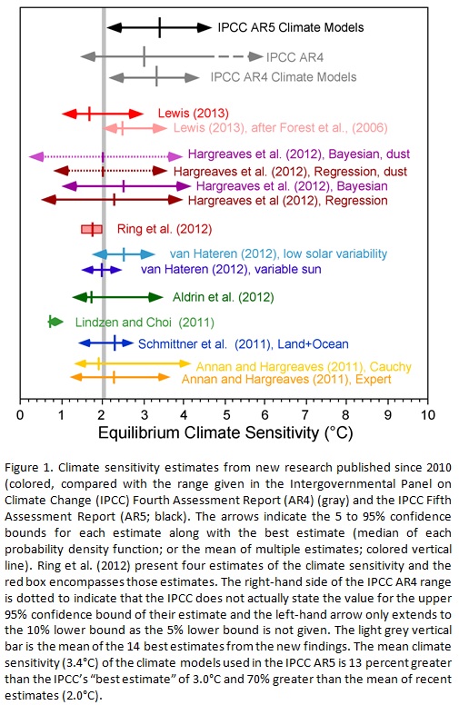
A comparison to various past estimates of ECS is made in figure 5. The base for figure 5 comes from the following weblink :
http://www.cato.org/sites/cato.org/files/wp-content/uploads/gsr_042513_fig1.jpg
See link for the original figure.

Figure 5 : Comparison of the results of this study (1.8) to other recent ECS estimates.
The estimate derived from this study agrees very closely with other recent studies. The gray line on figure 5 at a value of 2.0 represents the mean of 14 recent studies. Looking at the MSE curve in figure 4, 2.0 is essentially flat with 1.8 and would have a similar probability. This study further reinforces the conclusions of other recent studies which suggest climate sensitivity to CO2 is low relative to IPCC estimates .
The big difference with this study is that it is strictly based on the observed data. There are no models involved and only one assumption – that the longer period variation in temperature is driven by CO2 only. Given that the conclusion of a most likely sensitivity of 1.8 ° C / doubling is based on 163 years of observed data, the conclusion is likely to be quite robust.
A brief discussion of the assumption will now be made in light of the conclusion. The question to be asked is : If there are other factors affecting the long period trend of the observed temperature trend (there are many other potential factors, none of which will be discussed in this paper), what does that mean in terms of this best fit ECS curve ?
There are 2 options. If the true ECS is higher than 1.8, by definition , to match the observed data, there has to be some sort of negative forcing in the climate system pushing the temperature down from where it would be expected to be. In this scenario, CO2 forcing would be preventing the temperature trend from falling and is providing a net benefit.
The second option is the true ECS is lower than 1.8. In this scenario, also by definition, there has to be another positive forcing in the climate system pushing the temperature up to match the observed data. In this case CO2 forcing is smaller and poses no concern for detrimental effects.
For both of these options, it is hard to paint a picture where CO2 is going to be significantly detrimental to human welfare. The observed temperature and CO2 data over the last 163 years simply doesn’t allow for it.
Conclusion :
Based on data sets over the last 163 years, a most likely ECS of 1.8 ° C / doubling has been determined. This is a simple calculation based only on data , with no complicated computer models needed.
An ECS value of 1.8 is not consistent with any catastrophic warming estimates but is consistent with skeptical arguments that warming will be mild and non-catastrophic. At the current rate of increase of atmospheric CO2 (about 2.1 ppm/yr), and an ECS of 1.8, we should expect 1.0 ° C of warming by 2100. By comparison, we have experienced 0.86 ° C warming since the start of the HADCRUT4 data set. This warming is similar to what would be expected over the next ~ 100 years and has not been catastrophic by any measure.
For comparison of how unlikely the catastrophic scenario is, the IPCC AR5 estimate of 3.4 has an MSE error nearly as large as assuming that CO2 has zero effect on atmospheric temperature (see fig. 4).
There had been much discussion lately of how the climate models are diverging from the observed record over the last 15 years , due to “the pause”. All sorts of explanations have been posited by those supporting a high ECS value. The most obvious resolution is that the true ECS is lower, such as concluded in this paper. Note how “the pause” brings the observed temperature curve right to the 1.8 ECS synthetic record (see fig. 3). Given an ECS of 1.8, the global temperature is right where one would predict it should be. No convoluted explanations for “the pause” are needed with a lower ECS.
The high sensitivity values used by the IPCC , with their assumption that long term temperature trends are driven by CO2, are completely unsupportable based on the observed data. Along with that, all conclusions of “climate change” catastrophes are also completely unsupportable because they have the high ECS values the IPCC uses built into them (high ECS to get large temperature changes to get catastrophic effects).
Furthermore and most importantly, any policy changes designed to curb “climate change” are also unsupportable based on the data. It is assumed that the need for these policies is because of potential future catastrophic effects of CO2 but that is predicated on the high ECS values of the IPCC.
Files:
I have also attached a spreadsheet with all my raw data and calculations so anyone can easily replicate the work.
ECS Data (xlsx)
=============================================================
About Jeff:
I have followed the climate debate since the 90s. I was an early “skeptic” based on my geologic background – having knowledge of how climate had varied over geologic time, the fact that no one was talking about natural variation and natural cycles was an immediate red flag. The further I dug into the subject, the more I realized there were substantial scientific problems. The paper I am submitting is a paper I have wanted to write for years , as I did the basic calculations several years ago & realized there was no support in the observed data for high climate sensitivity.
“Temperature change as a function of CO2 concentration is a logarithmic function”
May be approximated by a log function over some range, but logarithms are unbounded, whereas energy absorption by CO2 must be bounded. At some point doublings should produce less increase in temp, eventually down to none.
Alex Hamilton.
I’ve been saying much the same thing about the lapse rate for some time.
@RichardLH
Correct curve fitting depends on high the correlation coefficient is. Anything below 0.5 is not significant and might be meaningless.
If it is higher than 0.99 you know that you have got it right. The binomial for the drop in maxima was 0.995 but still I decided that that was not the best fit….although I could use that fit to determine that 1972 was the turning point.
Somebody mentioned that it must be an a-c curve
I agreed, as otherwise we will all freeze to death….soon.
perhaps you should try to capture what I said before my tables begin?
Linear curve fitting is done to show a direction, from what we know is chaotic system, but most probably dependant on cycles. The slope shows the average change over time.
Would you agree with me that it is cooling in Alaska?
http://oi40.tinypic.com/2ql5zq8.jpg
(from 1998 it is cooling in Alaska at an average rate of -0.55 degrees C /decade)
Given that the temperature record seems to be continually adjusted (some may say tampered with) to effectively cool the past and warm the present, then this estimate of climate sensitivity to CO2 is likely to be an over-estimate.
Moreover, other work published on this site: http://wattsupwiththat.com/2010/03/08/the-logarithmic-effect-of-carbon-dioxide/
would also suggest that the ealier years of the graph would skew the result towards a higher estimate of sensitivity, given we might expect any further impact of increased CO2 emissions to be lower than for say 1850 to 2014.
In addition, we should expect US financial markets to relate more to temp than CO2 because of the heat island effect and agriculture affecting land temperature. The very near surface GHG concentrations probably also relate to economic activity (water vapor). I bet the relationship is stronger with surface station data than satellite.
Jeff,
How does your analysis and assumptions jive with what we do know about climate sensitivity?
We know that we get about 340 W/m^2 average power coming into the atmosphere and that about 30% is reflected/scattered away, leaving 70% to be absorbed which leaves us with 239 W/m^2 average that does get absorbed and must be balanced with what is radiated away from Earth. The average T of Earth is about 288.2K which leads to a surface emission of about 390 W/m^2 (stefan’s law).
Since what is radiated must be about 239 and what leaves the surface is 390, the atmosphere must absorb 390-239 =~ 150 W/m^2 over and above what it emits to space. Also, if we had an albedo of 0.30 without an atmosphere blocking any outgoing surface radiation, our mean surface temperature would have to be ~ 255K. That gives us an average sensitivity of (288-255) / 150 W/m^2 = 33/150 = 0.22 Deg C per W/m^2. Also, having an atmosphere ‘block’ 150 W/m^2 out of 390 W/m^2 means that about 62% of surface radiation (including what the atmosphere radiates beyond what it absorbs) actually makes it into space through the atmosphere.
Analysis of CO2 absorption in the standard atmosphere (clear skies only) results in about 3.7 W/m^2 increased atmospheric absorption for a doubling from around 370 ppm. This leads to a co2 doubling sensitivity of about 0.8 deg C.
Doing a small perturbation to T – increasing the surface T to compensate for the added co2 absorption we’d need 3.7/62% = 6 W/m^2 additional leaving the surface. This corresponds to 289.7 K average T versus 288.2 K or a rise of ~ 1.5 deg C. This is using Stefan’s law and the amount of power increase (assuming clear skies again) needed to balance a slightly more opaque atmosphere. If we apply the 0.22 sensitivity number, we see that 6W/m^2 would only need an increase of 1.3 deg C. The difference suggests a negative feedback. However, the 3.7 W/m^2 co2 factor is only valid for clear skies and less than half of the sky is clear as cloud cover tends to run close to 62%.
The catastrophic gw bunk comes from hansen and his pals. While they like to claim their fancy global coupled models are showing us the warming, reading the fine print shows something a bit different. Turns out they are using one dimensional modelling and assumptions, some perhaps dubious, about the details of clouds. Essentially, they exaggerate the results and assumptions always in the direction of more warming. Their warming comes from the resulting conclusion that added co2 and warmer conditions will result in more water vapor in the air but fewer clouds being formed. This means that since cloud cover drops with lower T, it must also drop with higher T and that means that Earth can never have 100% h2o vapor cloud cover if you are to believe hansen and his pal lacis, the 1-d modeling guy.
BTW, water vapor is quite similar to co2 in effect – both are virtually log factors with h2o being about twice the total effect and twice the effect of doubling. That means slight increases in h2o vapor content have very little effect and the shift of RH over small temperature ranges is also quite small. That is doubling does get you around 2 – 2 1/2 times the effect of co2 but a 5 deg C rise in atmospheric column temperature doesn’t get you beyond a 30% increase in absolute humidity (what counts) keeping the RH constant. Consequently, h2o cannot provide the killer positive feedback needed to raise the T.
Meanwhile, back at the ranch – we have no acceptable record of Earth’s albedo to come close to comparing with the TSI records. However, the factor that really counts is power absorbed, TSI * (1 – albedo), not TSI. Even more unfortunate is unlike Mars or the Moon, our albedo is 75% dependent on clouds and atmospheric factors and only around 25% dependent upon the surface – which is over 2/3 water. You can tell where these CAGW clowns are from when they spout off about albedo variations mostly being caused by human induced land use changes.
Paul_K says:
February 13, 2014 at 10:47 pm
@Michael D Smith says:
February 13, 2014 at 9:35 pm
Michael, whatever it is that you are doing, you are doing it incorrectly or you are using some very funny data. The net flux balance definitionally for a cumulative forcing, F(t), is given by:
Net flux imbalance = N(t) = F(t) – lambda*T
where lambda = the total feedback term = the inverse of the unit climate sensitivity
The common assumption is that all of the accumulated energy ends up in the oceans so the integral of the LHS (or RHS )= ocean heat
You can’t just integrate the forcing and assume that it all goes in as ocean heat, which I suspect is what you are doing. Many people, including respected sceptical scientists have used this equation to estimate lambda using data from the period you reference. Typically it yields a value of lambda of around 2.2 Watts/m2/deg C, equivalent to a unit climate sensitivity of 1/2.2 = 0.4 deg C/W/m2, equivalent to an ECS of around 1.6 deg C. If you use low forcing data or high ocean heat estimates, you can get to 2 deg C for a doubling. You can’t get to the numbers you are suggesting without using funny data or a funny governing equation.
I didn’t assume that it all went in as ocean heat. I determined that only 66.4% of it went in as ocean heat, as measured by temperature changes since 1957. This means that 33.6% did not. This means that 33.6% of the direct forcing was not absorbed by the system, which means it did not enter the system, (it was probably reflected / radiated by the increased cloud cover needed to reject the heat), or it has already left.
We have the direct forcing as 3.7W/m^2 per doubling of CO2 http://www.ipcc.ch/publications_and_data/ar4/wg1/en/ch2s2-3.html . 1.24W/m^2 of that since 1957 is not accounted for, and it’s a travesty™ that it isn’t. That is negative feedback. The imbalance right now, as measured by the accumulation of energy in the oceans, is only 0.5W/m^2. 0.5W/m^2, by anyone’s wildest estimate, is not enough to present a threat.
Unless perhaps you can show me that the imbalance that produces accumulation of energy in the system at 0.5W/m^2 is somehow not 0.5W/m^2.
I disagree. That is not where the real argument is.
The CAGW theory assumes that humidity and clouds amplify the warming due to CO2 by a factor of three: extra CO2 warms the ocean surface, causing more evaporation and extra humidity. Water vapor, or humidity, is the main greenhouse gas, so this causes even more surface warming. You can also add in the energy transport from latent heat of evaporation and convection too. So all these effects are bundled up and shoved under the rug called CO2 effect.
It is clearly stated by Rich Green a physical chemist:
This thinking is backed up by NASA:
Two of the most important drivers of the earth’s climate are the sun and water, yet the backa$$wards thinking of these CAGW modelers is that a miniscule addition to the amount of CO2 in the atmosphere (~40ppm) is DRIVING 1,386,000,000 cubic kilometers (332,519,000 cubic miles) of water.
RichardLH says:
February 14, 2014 at 2:47 am
Michael D Smith says:
February 13, 2014 at 9:35 pm
“…”
You want to estimate how close to the required Nyquist sampling intervals (time and space) that you are for that “Ocean Heat Measurement” figure you plugged into the spreadsheet?
Just a rough estimate will do. Or was that just a wild guess?
Well, I don’t think we’re going to resolve MHz signals in it. Did you think I was going to go and measure ocean heat myself?
But I would be very interested to hear why you think it will make a material difference over 55 years.
Here is a lesson. If you want to argue that sensitivity as a metric makes no sense or makes unwarranted assumptions.. nobody is going to listen to you. Thats voice in the wilderness stuff. You are outside the tent pissing in.
Steve, sadly, sensitivity as a metric makes no sense and makes unwarranted assumptions, whether or not anybody listens to me.
What sensitivity “should” be is the partial integral of the partial derivative of the global average temperature with respect to the carbon dioxide concentration. What sensitivity “is” is the voodoo-estimated global average temperature anomaly expected in the year 2100 from all causes. It is, in other words, completely misnamed, and for all practical purposes not computable.
Not computable? Did I say that? Sure I did. First of all, one cannot compute the global average temperature anomaly, not even with GCMs. One can only compute the global average (surface or otherwise) temperature, in degrees Kelvin. None of the physics — the Navier-Stokes equation, the various full-spectrum radiation formulae, phase transitions and albedo, latent heat, cloud dynamics — runs on any sort of “anomaly”. It requires initialization from and subsequently computes the temperature field, in depth, for every (silly) latitude/longitude pseudocartesian cell on the extremely non-flat surface of the globe for as many layers/slabs as the model descends into the ocean and into the atmosphere in addition to the “surface”.
The problem is, we do not know the temperature field. We do not know the actual average surface temperature of the planet within one whole degree Kelvin either way, and our knowledge of the surface temperature is better than our knowledge of the temperature field in depth. Perturbed parameter ensemble runs of the various CMIP5 models fairly clearly indicate that the future 100 year integrations of climate are highly “sensitive” to tiny perturbations of the initial conditions in degrees Kelvin, ones that more or less preserve some assumed starting temperature. They don’t even begin to explore the true range of uncertainty in just the initial temperature field, and one imagines that differences in the average of a degree might make major differences in 2100 absolute temperature prediction.
Finally, we have no way if “separating” the so-called sensitivity in the anomaly into natural vs anthropogenic components, because we do not know how to hindcast even the last 155 years with the models of CMIP5. They collectively fail to hindcast HADCRUT4 (with many of them failing worse than others, but none of them doing particularly well). CMIP5 completely misses the entire mostly natural cooling/warming pattern of the early 20th century, so it is not really that surprising that it overattributes the nearly identical warming of the late 20th century to anthropogenic cases.
Maybe. We really don’t know. The errors in HADCRUT4 or the other surface temperature measures are substantial and grow rapidly as one goes back in the past. Perhaps the CMIP5 MME mean is — inexplicably, given its complete lack of theoretical statistical foundation — dead on the money and it is HADCRUT, GISS, and so on that are wrong. Eventually the future will play out and maybe we will learn, just as we’ve been learning from the entire interval after the CMIP5 reference period (and before the reference period) that the CMIP5 models are failing badly — so far.
However, model by model, the prediction of the mean global average surface temperature in 2100 is not sensitivity to anthropogenic CO_2 because it contains an unknown admixture of natural warming and, in general, the models one at a time are doing a terrible job at predicting almost the entire climate period outside of their reference (training) set. The models themselves tell us that they cannot be trusted to the extent that we can compare their predictions to actual data. At this time we Do Not Know if the climate is very insensitive to additional CO_2, with natural feedbacks largely cancelling, or if The Hansen Story is true, and natural feedbacks strongly augment the warming due to additional CO_2. We don’t even know if either scenario is written in stone, or if one or the other are equally possible due to vagrant random fluctuations or unknown internal dynamics associated with e.g. decadal oscillations or in the event that there really is some sort of connection between solar state and climate outside of the small variation in direct forcing.
We do know that Hansen’s oft-and-highly-publicly-stated beliefs in extreme “sensitivity” (or total warming from all sources and causes) are probably wrong at this point — the actual climate is way off the tracks that any of the models that come close to this extreme sensitivity produce when their initial conditions are perturbed. We even know that the CMIP5 MME mean is probably wrong at this point, and that the total warming from all sources is going to end up being less than the 2.7ish degrees C it produces, understandably since it still contains all of the egregiously failed CMIP5 models in its equally weighted average. AR5, chapter 9, admits all of this — while carefully omitting any mention of the uncertainties in the SPM and “magically” transforming a mean that has no meaning whatsoever derived from the theory of statistics into “confidence” in the SPM.
In the end, as a matter of fact, we don’t know what the climate will do in/by 2100. We don’t even have a good idea.
rgb
Windchasers says:
February 14, 2014 at 8:14 am
IF (CPI is the only driver of temperature) THEN (sensitivity [to CPI] is low)
IF (CPI is not the only driver [or not one at all] of temperature) THEN (CPI isn’t harmful [wrt GAST])
Except it’s not right. Say the natural variations (or other forcings) were in the downward direction, so that the CO2 sensitivity is higher than expected.
Does this mean that future CO2 emissions won’t be harmful? No. That’s true only if you think that the downward variations are going to strengthen to compensate for the increased CO2. IOW, all that Joe showed is that the past CO2 emissions may have been helpful or neutral, not that future emissions will also be.
———————————————————————————————————————-
That’s a fair point but the past 17 years of the observational record suggest otherwise.
If the correct situation is that “other factors cool” then, for about 2 decades up to 1997, they were having less of an effect than the increase in CO2 because the overall trend was upwards. Since then they’ve (at least) matched the effect of further CO2 increase which would mean that, for the moment at least, they’re increasingly quite alarmingly in the strength of their cooling.
Natural cycles tend not to “switch” instantly, so having had 17 years of “the other” factors increasing their cooling effect it would be likely that we’d be facing at least a similar period of continued cooling even if they’d started to relent.
Dr Burns says: @ur momisugly February 13, 2014 at 2:53 pm
…..I wouldn’t be surprised if Law Dome has also been faked.
>>>>>>>>>>>>>>>
The CO2 data is as manipulated as the temperature data:
An example of present day manipulation, note the cherry picking of values, is outlined by Mauna Loa Obs. The Lab sits on top of an active volcano (fumes) near an ocean full of living things.
It is a very nice way to get a small standard deviation in your data and get rid of any pesky results that do not fit the ‘Cause’
This reminds me of the same manipulation we see in the temperature data where the temperature from the few and far between truly rural stations is adjusted UP to match the more plentiful airport and city stations.
HenryP Thanks, I copied your Alaska temp graph
HenryP, do you have temp graphs from other land masses bordering the Arctic Ocean?
I understand that the poles have less accurate measurements, including by satellite for various reasons. Although I think Ocean oscillations, in particular the Pacific are most significant contributors to ice melt and freezing, it would be interesting to see if there is a consistent lag between land temps and Arctic melt and freeze.
” rgbatduke says:
February 14, 2014 at 11:02 am
”
Robert,
Please take a look at my (slightly unwieldy) post of 2/14/2014 10:46 am and let me know if it mostly makes sense.
Bill Illis says: @ur momisugly February 13, 2014 at 4:05 pm
Mosher says “Hansen for example relies on Paleo data.”
Let’s take the last glacial maximum and Hansen’s estimates based on that (and he actually wrote a paper on it). Temps were -5.0C lower, CO2 was at 185 ppm….
>>>>>>>>>>>>>>>>>>
If the CO2 was really 185 ppm during the ast glacial maximum then we would not be here. (Based on the ASSumption of CO2 is uniform throughout the atmosphere.)
Bill Illis says: @ur momisugly February 13, 2014 at 4:05 pm
Here are plants at different CO2 levels:
http://i32.tinypic.com/nwix4x.png
http://wattsupwiththat.files.wordpress.com/2012/06/image_thumb4.png?w=625&h=389
(Remember a plant has to have enough CO2 to support seed production and not just to survive.)
“Does this mean that future CO2 emissions won’t be harmful? No. That’s true only if you think that the downward variations are going to strengthen to compensate for the increased CO2. IOW, all that Joe showed is that the past CO2 emissions may have been helpful or neutral, not that future emissions will also be.”
This is true but you need to consider what its likely to mean in the context of the next century or two. There’s a plank to CGW that is often missed- not only does it have to be caused by man-made carbon, and harmful, and catastrophic.. it needs to be so in a timeframe whereby heavy CO2 production both remains essential to human society, and technology hasnt advanced enough to either neutralize or mitigate the CO2 or its effects. IE- even a 1:1 ECS would be catastrophic over a long enough time frame (for that matter cotton candy production would be catastrophic over a long enough time frame). What a manageable ECS tells us is that there won’t likely be catastrophic (or even harmful) results in the timeframe such that it matters. Even without considering the advance of technology, fossil fuels would eventually diminish thereby diminishing CO2 production. That tells us that there is a finite volume of CO2 production in our future. The only thing relevant is if some concentration in the next century or two is truly dangerous. But the idea that we’ll be burning coal in 200 years is hard to swallow… barring some bigger catastrophe that sets civilization back (or perhaps some economic lunacy). The analogy of shutting down 18th century NYC out of concern for mounting piles of horse dung given population projections is always cogent.
With warmists, you always have to keep your eye on the ball. Catastrophic global warming is the only warming that means anything to anyone but climate scientists.
HenryP says:
February 14, 2014 at 9:57 am
“RichardLH
Correct curve fitting depends on high the correlation coefficient is. Anything below 0.5 is not significant and might be meaningless.
If it is higher than 0.99 you know that you have got it right. The binomial for the drop in maxima was 0.995 but still I decided that that was not the best fit….although I could use that fit to determine that 1972 was the turning point.”
Assuming you have any clue as to what the underlying period functions and the min and max that apply to their frequencies are – sure. But you don’t so you can’t.
“Would you agree with me that it is cooling in Alaska?”
I would agree that it has cooled in Alaska over the period in question. However that says nothing at all about what will happen next. It could go 45 degree upwards from now on!
Linear functions are only valid over the range they are drawn from. All the rest is illusion.
Michael D Smith says:
February 14, 2014 at 10:58 am
“Well, I don’t think we’re going to resolve MHz signals in it. Did you think I was going to go and measure ocean heat myself?”
Not really, but you shouldn’t assume that others have done it to the required accuracy for you either. Nyquist applies to all fields and sampling distances in time and space, from MHz to Millennia, and from mm to 1000’s km.
If you want to determine a field and the changes in that field (which is what you need) then you have to sample that field above the Nyquist rate or it is all just guesswork.
“But I would be very interested to hear why you think it will make a material difference over 55 years.”
Because if you do not know the field and how it has changed in time you cannot derive an average that says how much heat has moved and in which direction over, say, 55 years.
richardLH says
I would agree that it has cooled in Alaska over the period in question. However that says nothing at all about what will happen next.
Henry say
I know what will happen next: global cooling until around 2040
http://blogs.24.com/henryp/2012/10/02/best-sine-wave-fit-for-the-drop-in-global-maximum-temperatures/
I don’t think I can give you more clues.
@darrylb
darryl, we are cooling from the top [90] latitude down, as my results from Alsaka clearly show,
and also from the other side, e.g.
http://wattsupwiththat.com/2013/10/22/nasa-announces-new-record-growth-of-antarctic-sea-ice-extent/#more-96133
I only have the results of the stations reported in my tables, and it only shows the slopes (the linear trend) over the specific periods mentioned, that is the speed of change over the specific period observed.
Basiccally I only trust my own data, as I can provide proof of tampering of the results coming from Gibraltar. Since then, I distrust anglo saxon stations, generally…
Whatever you do to data (measurement results) you do not “correct” them..
The satelites data sets also worry me. I don’t understand how they calibrate and I suspect that the temp.(“zero”) in our solar system might not be unmovable (is it about 0.285 K?). It might shift. So I don’t know how they figured that problem out.
As I always say in science, don’t trust anyone but yourself.
Assuming the formula for deltaT is ok , there’s nothing wrong with the ECS curves. I’m not sure the observed ‘curve’ provides a valid comparison, though, since it is that which is measuring the instantaneous response to CO2 at ~400 ppm.
I don’t have any reason to criticize Jeff’s analysis; he explains what he did.
I have a basic distrust of particularly the HadCRUT data set, that is I don’t believe the data itself. John Christy et al showed that ocean water and ocean air temperatures are not the same and are not correlated (why would they be, given ocean currents and wind speeds).
So I don’t believe any data earlier than about 1980 when the Ocean floating buoys were put out there, or thereabouts.
And I also believe that the ocean evap / vapor / cloud /precip water cycle is in full negative feedback control of the whole system; which doesn’t mean there is no variation; just no catastrophic consequence. The system forward amplifier gain (if any) cannot be very high, so we can’t expect the stability common with electronic feedback systems.
Peter Humbug did an experiment on his play station where he removed ALL of the water from the atmosphere; so no vapor, and no clouds, and then let his gizmo run. He got all the water back in three months. As I recall he reported this in a peer reviewed paper in SCIENCE, but I may have the wrong journal. (I actually read his paper in the Journal). I think he would have had the same result if he had removed all of the CO2 as well.
I don’t believe that the earth would be a frozen ice ball if it had no atmospheric CO2.
My reason is that the solar blow torch that warms the earth is 1366 W/m^2, NOT 342 W/m^2, and at the surface, that becomes maybe 1,000 W/m^2, not 250 W/m^2.
Maybe after sunset, the dark earth is radiation all the time at whatever Trenberth’s number is, but during the daylit hours, when the surface is being cooked by 1,000-1366 W/m^2, it is also hotter and simultaneously radiating much more than 390 W/m^2 for a 288 K black body rate.
Take ALL of the GHG out of the atmosphere and the ground level TSI, would be closer to 1366 W/m^2, (less blues sky scattered), and we would get bags of water in the atmosphere in a big hurry; even if you started with a frozen ice ball.
You seem remarkably confident. Why don’t you try and make a bit of money from your predictions. There are plenty of warmers who are happy to bet on future temperature change over various timescales. Unfortunately , too few sceptics are prepared to take them on. I am sceptical of catastrophic global warming but I still expect modest warming over the next few decades.