This exercise in data analysis pins down a value of 1.8C for ECS.
Guest essay by Jeff L.
Introduction:
If the global climate debate between skeptics and alarmists were cooked down to one topic, it would be Equilibrium Climate Sensitivity to CO2 (ECS) , or how much will the atmosphere warm for a given increase in CO2 .
Temperature change as a function of CO2 concentration is a logarithmic function, so ECS is commonly expressed as X ° C per doubling of CO2. Estimates vary widely , from less than 1 ° C/ doubling to over 5 ° C / doubling. Alarmists would suggest sensitivity is on the high end and that catastrophic effects are inevitable. Skeptics would say sensitivity is on the low end and any changes will be non-catastrophic and easily adapted to.
All potential “catastrophic” consequences are based on one key assumption : High ECS ( generally > 3.0 ° C/ doubling of CO2). Without high sensitivity , there will not be large temperature changes and there will not be catastrophic consequences. As such, this is essentially the crux of the argument : if sensitivity is not high, all the “catastrophic” and destructive effects hypothesized will not happen. One could argue this makes ECS the most fundamental quantity to be understood.
In general, those who are supportive of the catastrophic hypothesis reach their conclusion based on global climate model output. As has been observed by many interested in the climate debate, over the last 15 + years, there has been a “pause” in global warming, illustrating that there are significant uncertainties in the validity of global climate models and the ECS associated with them.
There is a better alternative to using models to test the hypothesis of high ECS. We have temperature and CO2 data from pre-industrial times to present day. According to the catastrophic theory, the driver of all longer trends in modern temperature changes is CO2. As such, the catastrophic hypothesis is easily tested with the available data. We can use the CO2 record to calculate a series of synthetic temperature records using different assumed sensitivities and see what sensitivity best matches the observed temperature record.
The rest of this paper will explore testing the hypothesis of high ECS based on the observed data. I want to re-iterate the assumption of this hypothesis, which is also the assumption of the catastrophists position, that all longer term temperature change is driven by changes in CO2. I do not want to imply that I necessarily endorse this assumption, but I do want to illustrate the implications of this assumption. This is important to keep in mind as I will attribute all longer term temperature changes to CO2 in this analysis. I will comment at the end of this paper on the implications if this assumption is violated.
Data:
There are several potential datasets that could be used for the global temperature record. One of the longer and more commonly referenced datasets is HADCRUT4, which I have used for this study (plotted in fig. 1) The data may be found at the following weblink :
http://www.cru.uea.ac.uk/cru/data/temperature/HadCRUT4-gl.dat
I have used the annualized Global Average Annual Temperature anomaly from this data set. This data record starts in 1850 and goes to present, so we have 163 years of data. For the purposes on this analysis, the various adjustments that have been made to the data over the years will make very little difference to the best fit ECS. I will calculate what ECS best fits this temperature record, given the CO2 record.

Figure 1 : HADCRUT4 Global Average Annual Temperature Anomaly
The CO2 data set is from 2 sources. From 1959 to present, the Mauna Loa annual mean CO2 concentration is used. The data may be found at the following weblink :
ftp://aftp.cmdl.noaa.gov/products/trends/co2/co2_annmean_mlo.txt
For pre-1959, ice core data from Law Dome is used. The data may be found at the following weblink :
ftp://ftp.ncdc.noaa.gov/pub/data/paleo/icecore/antarctica/law/law_co2.txt
The Law Dome data record runs from 1832 to 1978. This is important for 2 reasons. First, and most importantly, it overlaps Mauna Loa data set. It can easily be seen in figure 2 that it is internally consistent with the Mauna Loa data set, thus providing higher confidence in the pre-Mauna Loa portion of the record. Second, the start of the data record pre-dates the start of the HADCRUT4 temperature record, allowing estimates of ECS to be tested against the entire HADCRUT4 temperature record. For the calculations that follow, a simple splice of the pre-1959 Law Dome data onto the Mauna Loa data was made , as the two data sets tie with little offset.

Figure 2 : Modern CO2 concentration record from Mauna Loa and Law Dome Ice Core.
Calculations:
From the above CO2 record, a set of synthetic temperature records can be constructed with various assumed ECS values. The synthetic records can then be compared to the observed data (HADCRUT4) and a determination of the best fit ECS can be made.
The equation needed for the calculation of the synthetic temperature record is as follows :
∆T = ECS* ln(C2/C1)) / ln(2)
where :
∆T = Change in temperature, ° C
ECS = Equilibrium Climate Sensitivity , ° C /doubling
C1 = CO2 concentration (PPM) at time 1
C2 = CO2 concentration (PPM) at time 2
For the purposes of this test of sensitivity, I set time 1 to 1850, the start of the HADCRUT4 temperature dataset. C1 at the same time from the Law Dome data set is 284.7 PPM. For each year from 1850 to 2013, I use the appropriate C2 value for that time and calculate ∆T with the formula above. To tie back to the HADCRUT4 data set, I use the HADCRUT4 temperature anomaly in 1850 ( -0.374 ° C) and add on the calculated ∆T value to create a synthetic temperature record.
ECS values ranging from 0.0 to 5.0 ° C /doubling were used to create a series of synthetic temperature records. Figure 3 shows the calculated synthetic records, labeled by their input ECS, as well as the observed HADCRUT4 data.

Figure 3: HADCRUT4 Observed data and synthetic temperature records for ECS values between 0.0 and 5.0 ° C / doubling. Where not labeled, synthetic records are at increments of 0.2 ° C / doubling. Warmer colors are warmer synthetic records.
From Figure 3, it is visually apparent that a ECS value somewhere close to 2.0 ° C/ doubling is a reasonable match to the observed data. This can be more specifically quantified by calculating the Mean Squared Error (MSE) of the synthetic records against the observed data. This is a “goodness of fit” measurement, with the minimum MSE representing the best fit ECS value. Figure 4 is a plot of MSE values for each ECS synthetic record.

Figure 4 : Mean Squared Error vs ECS values. A few ECS values of interest are labeled for further discussion
In plotting, the MSE values, a ECS value 1.8 ° C/ doubling is found to have the minimum MSE and thus is determined to be the best estimate of ECS based on the observed data over the last 163 years.
Discussion :
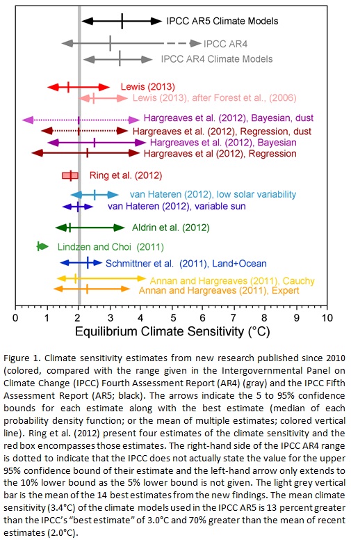
A comparison to various past estimates of ECS is made in figure 5. The base for figure 5 comes from the following weblink :
http://www.cato.org/sites/cato.org/files/wp-content/uploads/gsr_042513_fig1.jpg
See link for the original figure.

Figure 5 : Comparison of the results of this study (1.8) to other recent ECS estimates.
The estimate derived from this study agrees very closely with other recent studies. The gray line on figure 5 at a value of 2.0 represents the mean of 14 recent studies. Looking at the MSE curve in figure 4, 2.0 is essentially flat with 1.8 and would have a similar probability. This study further reinforces the conclusions of other recent studies which suggest climate sensitivity to CO2 is low relative to IPCC estimates .
The big difference with this study is that it is strictly based on the observed data. There are no models involved and only one assumption – that the longer period variation in temperature is driven by CO2 only. Given that the conclusion of a most likely sensitivity of 1.8 ° C / doubling is based on 163 years of observed data, the conclusion is likely to be quite robust.
A brief discussion of the assumption will now be made in light of the conclusion. The question to be asked is : If there are other factors affecting the long period trend of the observed temperature trend (there are many other potential factors, none of which will be discussed in this paper), what does that mean in terms of this best fit ECS curve ?
There are 2 options. If the true ECS is higher than 1.8, by definition , to match the observed data, there has to be some sort of negative forcing in the climate system pushing the temperature down from where it would be expected to be. In this scenario, CO2 forcing would be preventing the temperature trend from falling and is providing a net benefit.
The second option is the true ECS is lower than 1.8. In this scenario, also by definition, there has to be another positive forcing in the climate system pushing the temperature up to match the observed data. In this case CO2 forcing is smaller and poses no concern for detrimental effects.
For both of these options, it is hard to paint a picture where CO2 is going to be significantly detrimental to human welfare. The observed temperature and CO2 data over the last 163 years simply doesn’t allow for it.
Conclusion :
Based on data sets over the last 163 years, a most likely ECS of 1.8 ° C / doubling has been determined. This is a simple calculation based only on data , with no complicated computer models needed.
An ECS value of 1.8 is not consistent with any catastrophic warming estimates but is consistent with skeptical arguments that warming will be mild and non-catastrophic. At the current rate of increase of atmospheric CO2 (about 2.1 ppm/yr), and an ECS of 1.8, we should expect 1.0 ° C of warming by 2100. By comparison, we have experienced 0.86 ° C warming since the start of the HADCRUT4 data set. This warming is similar to what would be expected over the next ~ 100 years and has not been catastrophic by any measure.
For comparison of how unlikely the catastrophic scenario is, the IPCC AR5 estimate of 3.4 has an MSE error nearly as large as assuming that CO2 has zero effect on atmospheric temperature (see fig. 4).
There had been much discussion lately of how the climate models are diverging from the observed record over the last 15 years , due to “the pause”. All sorts of explanations have been posited by those supporting a high ECS value. The most obvious resolution is that the true ECS is lower, such as concluded in this paper. Note how “the pause” brings the observed temperature curve right to the 1.8 ECS synthetic record (see fig. 3). Given an ECS of 1.8, the global temperature is right where one would predict it should be. No convoluted explanations for “the pause” are needed with a lower ECS.
The high sensitivity values used by the IPCC , with their assumption that long term temperature trends are driven by CO2, are completely unsupportable based on the observed data. Along with that, all conclusions of “climate change” catastrophes are also completely unsupportable because they have the high ECS values the IPCC uses built into them (high ECS to get large temperature changes to get catastrophic effects).
Furthermore and most importantly, any policy changes designed to curb “climate change” are also unsupportable based on the data. It is assumed that the need for these policies is because of potential future catastrophic effects of CO2 but that is predicated on the high ECS values of the IPCC.
Files:
I have also attached a spreadsheet with all my raw data and calculations so anyone can easily replicate the work.
ECS Data (xlsx)
=============================================================
About Jeff:
I have followed the climate debate since the 90s. I was an early “skeptic” based on my geologic background – having knowledge of how climate had varied over geologic time, the fact that no one was talking about natural variation and natural cycles was an immediate red flag. The further I dug into the subject, the more I realized there were substantial scientific problems. The paper I am submitting is a paper I have wanted to write for years , as I did the basic calculations several years ago & realized there was no support in the observed data for high climate sensitivity.
According to the IPCC’s understanding of the failed models, the climate sensitivity parameter (the quantity in Kelvin per Watt per square meter by which the CO2 radiative forcing is multiplied to give the resultant global warming) has an instantaneous value 0.31 K/W/m2, rising to 0.44 K/W/m2 after 100 years, 0.5 K/W/m2 after 200 years and 0.88 K/W/m2 at equilibrium (after 1000-3000 years).
It is not clear to me what account the head posting takes of these imagined (and largely imaginary) variations in the climate-sensitivity parameter that are thought to be caused by the evolution of net-positive temperature feedbacks.
The feedbacks approximately triple the direct warming from CO2 or from any other cause, if the models are right, but the tripling occurs only after milllennia. None of the feedbacks can be directly measured; none can be indirectly determined by any theoretical method; and, even if they could, it is not possible clearly to distinguish the anthropogenic from the natural component in past global warming. And I do mean “past”: there has been no warming for 13 years, on the average of all five global temperature datasets.
I did not see any comments from the poster (correct me if I am wrong), but all he has done is to prove that which we already know: more heat causes more carbondioxide.
Any first year chemistry student knows that to make a water based standard solution you have to remove the carbondioxide by boiling.
Any (good) chemist knows that there are giga tons and giga tons of bi-carbonates dissolved in the oceans and that (any type of) warming would cause it to be released:
HCO3- + (more) heat => (more) CO2 (g) + OH-.
This is the actual reason we are alive today. Cause and effect, get it? There is a causal relationship. More warming naturally causes more CO2. It is not the other way around, as Al Gore alleges in his movie. Without warmth and carbon dioxide there would be nothing, really. To make that what we dearly want, i.e. more crops, more trees, lawns and animals and people, nature uses water and carbon dioxide and warmth, mostly. The fact that humanity adds a bit of carbon dioxide to the atmosphere is purely co-incidental, and appears to be beneficial, if you want to have a green world.
If you want to prove that, in its turn, more carbondioxide also “produces” or “retains” more heat, you could follow the procedure that I have done, namely,
I first studied the mechanism by which AGW is supposed to work. I will spare you all the scientific details. However, if you are interested you can read some of my musings here:
http://blogs.24.com/henryp/2011/08/11/the-greenhouse-effect-and-the-principle-of-re-radiation-11-aug-2011/
I quickly figured that the proposed mechanism implies that more GHG would cause a delay in radiation being able to escape from earth, which then causes a delay in cooling, from earth to space, resulting in a warming effect.
It followed naturally, that if more carbon dioxide (CO2) or more water (H2O) or more other GHG’s were to be blamed for extra warming we should see minimum temperatures (minima) rising faster, pushing up the average temperature (means) on earth.
I subsequently took a sample of 47 weather stations, analysed all daily data, and determined the ratio of the speed in the increase of the maximum temperature (maxima), means and minima. I have reported my results here many times
You will find that if we take the speed of warming over the longest period (i.e. from 1973/1974) for which we have very reliable records,
we find the results of the speed of warming, maxima : means: minima
0.036 : 0.014 : 0.006 in degrees C/annum.
That is ca. 6:2:1. So it was maxima pushing up minima and means and not the other way around. Anyone can duplicate this experiment and check this trend in their own backyard or at the weather station nearest to you.
Interestingly enough, plotted against time, in places on earth where they chopped the trees (e.g. Argentina) I found minima dropping even further, below average. Where more green was planted (e.g. Las Vegas) I did find minima rising somewhat more than average.
So, what it showed me is that (more) nature naturally traps some (more) heat.
In so far as this can be termed “AGW”
perhaps yes, then,
if you mean with that people want more trees, more crops, more lawns, etc
then indeed this does trap some heat.
There is also clear eveidence that the biosphere has been booming since 1950.
But, please, please, don’t blame the poor carbon dioxide for the warming.
Nobody. Really. This is just so silliy, so wrong and unscientific. Tell me you agree.
HenryP says:
February 14, 2014 at 3:23 am
“But, please, please, don’t blame the poor carbon dioxide for the warming.
Nobody. Really. This is just so silliy, so wrong and unscientific. Tell me you agree.”
There are no current measurements of temperatures on a Global, historical, basis that allows the claim that CO2 is the cause of the warming to be proven beyond doubt.
That cuts both ways unfortunately.
As has been pointed out, this analysis assumes that the warming was caused entirely by CO2. So, based on this assumption, which warmists would certainly agree to, the warming over the rest of this century will be modest.
But the assumption is clearly nonsense, and almost certainly the figure of 1.8 degrees is also nonsense.
Despite increasing CO2 levels there has been no warming in this century. This strongly suggests that some natural processes are more significant than CO2, at least over this time period.
But the most damning evidence comes from the ice cores. They show that the CO2 follows the temperature, and not the other way around. As far as I’m aware, the ice cores do not provide the slightest evidence that CO2 can control the global temperature. If the sensitivity is around 2 degrees, why doesn’t it show up clearly in the ice core data?
So, here’s a challenge to anyone who believes the sensitivity is 1.8 degrees or higher: show me some historical data from before the 20th century that shows a change in CO2 that was followed by a corresponding change in temperature.
Chris
The Paleoclimate sensitivity as expressed in K/W/m2 is actually 0.0 K/W/m2 +/- 40.0 K/W/m2
… which would normally be thought of as a “null” or random result.
http://s15.postimg.org/4e2xjsjmj/Temp_C_Wm2_Making_Sense2012.png
I’m in the process of updating this to 2,500 datapoints but it is very computational intensive, I can only do about 30 datapoints at a time before the PC says it is overtaxed. Essentially back-fitting the high-res temperature line to the exact time that reliable CO2 estimates are available.
@RichardLH
1) but we don’t see minimum temperatures rising?
all three tables
http://blogs.24.com/henryp/2013/02/21/henrys-pool-tables-on-global-warmingcooling/
showed that the big cooler has come on, a few years before the end of the last milennium.
We must get the world off the CO2 horse now, and boldly announce that global cooling will rule in the next two to three decades.
2) I have thought long if one would be able to do an experiment to prove if the net effect of more CO2 is that of warming or cooling. Obviously you cannot use a closed box.
You have to assess both the cooling of the gas (by measuring deflected sunlight to space) and the warming of the gas (by deflecting earthshine to earth).
It seems impossible.
3) CO2 also causes cooling by taking part in the life cycle. Plants and trees need warmth and CO2 to grow – which is why you don’t see trees at high latitudes and – altitudes. It appears no one has any figures on how much this cooling effect might be. There is clear evidence that there has been a big increase in greenery on earth in the past 4 decades.
http://wattsupwiththat.com/2011/03/24/the-earths-biosphere-is-booming-data-suggests-that-co2-is-the-cause-part-2/
It seems that an awful lot of posters are trying to read far more into this than the author intended, despite his clear (to me, at least) explanation in a later post.
He is not trying to obtain a “correct” figure for the ECS. Nor is he claiming to acount for the myriad factors needed to do so, even if such a figure is meaningful (and static) in the first place.
His argument is really a very simple and logical one, based on two assumptions that he admits openly are likely to be invalid:
(1) CO2 concentration affects global average temperature by a simple logarithmic function
(2) No other factors affect global average temperature..
He also makes the common, implied, assumption that “global average temperature” has any sensible physical meaning or consequence. Unfortunately, that’s one that we all have to make if we’re to take an interest in questions of climate because the whole world and his dog has been told how vital it is. Just saying “it’s meaningless”may well be true, but it’s a truth that no-one’s going to hear no matter how loud you shout it.
Given those (admittedly faulty) assumtions, it’s entirely reasonable to “curve fit” because the assumptions themselves define global average temperature as a function of CO2:
(CO2 affects temperature) & (nothing else changes temperature) -> temperature = f(CO2)
is perfectly valid logic.
So, given those assumptions, a curve fit of CO2 against Temp will allow us to obtain an ECS that is valid within the assumptions . The figure he arrives at is 1.8 deg C per doubling.
He also then comments about the logical inferences possible if the main assumptions are incorrect, and other factors do also affect temperature:
(a) If the net effect of “other factors” is to reduce temperature then the global average temperature must be more sensitive to CO2 than calculated .but, without the CO2 increase to offset the other factors the world would now be cooling,l which makes CO2 very important unless we all want to freeze.
(b) If the net effect of “other factors” is to increase temperature then the global average temperature must be less sensitive to CO2 than calculated, which makes CO2 unimportant other than as plant food.
Note that, in (b), any simple feedbacks that might amplify the resulting small effect of CO2 to dangerous levels will similarly amplify the “other factors” so you can’t invoke feedbacks to make CO2 dangerous without also making the “other factors” dangerous.
The beauty of logic is that it often allows you to reach sound conclusions, very simply, and without sheaves of statistical manipulations that are prone to mistakes, abuse and general incompetence. In this case the conclusions are simple:
IF (CO2 is the only driver of temperature) THEN (sensitivity is low)
IF (CO2 is not the only driver of temperature) THEN (CO2 isn’t harmful)
Joe says:
February 14, 2014 at 5:24 am
“IF (CO2 is the only driver of temperature) THEN (sensitivity is low)
IF (CO2 is not the only driver of temperature) THEN (CO2 isn’t harmful)”
———————–
Summarized very nicely and spot on with the point I was trying to make & evidently didn’t communicate effectively given the myriad of posts thinking I was trying to make some larger point.
And why make this point at all ??
Because how many times have you heard warmist / catastrophists try to argue their point using this logic ? And how many times have you seen policy makers base their decisions essentially using the same logic ??? All the time on both accounts. This essay was put together only to show that by their own logic, there would be no problem. Most of the criticisms of the essay were about faulty logic, which was clearly stated & acknowledged at the beginning of the essay :
“I want to re-iterate the assumption of this hypothesis, which is also the assumption of the catastrophists position, that all longer term temperature change is driven by changes in CO2. I do not want to imply that I necessarily endorse this assumption, but I do want to illustrate the implications of this assumption.”
I don’t think I could have made that point much clearer.
And of course I do bring it full circle at the end indicating policy changes based on this logic are unwarranted….. because by their own logic, it doesn’t compute !
The reason I haven’t commented further on all the myriad of posts about faulty logic was that it was that those posters had missed the entire point of the paper & were talking about issues that I never intended to address BUT I want to assure you, I was readily aware of.
HenryP says:
February 14, 2014 at 5:11 am
“We must get the world off the CO2 horse now, and boldly announce that global cooling will rule in the next two to three decades.”
I would agree that the data appears to support your conclusion on a Global scale as well.
http://i29.photobucket.com/albums/c274/richardlinsleyhood/Fig8HadCrutGISSRSSandUAHGlobalAnnualAnomalies-Aligned1979-2013withGaussianlowpassandSavitzky-Golay15yearfilters_zps670ad950.png
though the data seems to suggest a more recent turning point. This is a S-G curve (similar to LOWESS) so it could change with new data but I do not think it will be a sharper curve than currently displayed. YMMV.
Joe says:
February 14, 2014 at 5:24 am
“It seems that an awful lot of posters are trying to read far more into this than the author intended, despite his clear (to me, at least) explanation in a later post.
…
IF (CO2 is the only driver of temperature) THEN (sensitivity is low)
IF (CO2 is not the only driver of temperature) THEN (CO2 isn’t harmful)”
Agreed. This is a UPPER level for sensitivity – not a central value.
Joe says:
February 14, 2014 at 5:24 am
It seems that an awful lot of posters are trying to read far more into this than the author intended
========
Agreed. The analysis is reasonable within the assumptions. Catastrophic warming is not supported by the data.
Steven Mosher writes-
“Hansen for example relies on Paleo data.”
As with all of his work product, Hansen cherry picks the bits he likes, adjusts everything within his reach, and poo-poo’s the rest.
Hansen’s use of Paleo data to support a high climate sensitivity was slammed almost 15 years ago.
As reported here by Anthony and friends-
http://wattsupwiththat.com/2011/11/28/senior-ncar-scientist-admits-quantifying-climate-sensitivity-from-real-world-data-cannot-even-be-done-using-present-day-data/
“date: Fri, 30 Jun 2000 12:30:43 -0600 (MDT)
from: Tom Wigley…
subject: Re: …
to: Keith Briffa…
Keith and Simon (and no-one else),
Paleo data cannot inform us *directly* about how the climate sensitivity
(as climate sensitivity is defined). Note the stressed word. The whole
point here is that the text cannot afford to make statements that are
manifestly incorrect. This is *not* mere pedantry. If you can tell me
where or why the above statement is wrong, then please do so.
Quantifying climate sensitivity from real world data cannot even be done
using present-day data, including satellite data. If you think that one
could do better with paleo data, then you’re fooling yourself. This is
fine, but there is no need to try to fool others by making extravagant
claims.”
Hansen also claims a TOA electromagnetic intensity imbalance by cherry picking his climate model, because the satellite observations do not provide the resolution needed to support his pre-ordained imbalance.
Hansen is a first rate activist of opportunity.
The atmosphere is gas.
Gas is the simplest phase of matter.
If you don’t have your gas mechanics down
you’re going to be a failure anywhere energy and matter
are discussed.
CO2 sensitivity people were wrong.
The only thing keeping it alive is the same bad judgement
that got them believing it was anything but a canard fronting a scam in the first place.
Nice summary Henry P-
IF (CO2 is the only driver of temperature) THEN (sensitivity is low)
IF (CO2 is not the only driver of temperature) THEN (CO2 isn’t harmful)
The exception, not noted, is if the unaccounted for, other drivers are negative and temporary.
The PDO is an example that we understand better than most. It’s in its negative phase and probably, IMO, masking the GHG forcing. We can look at the 1942-1978 and earlier time periods when the negative phase of the PDO, presumably, forced temporary global cooling. Jeff L. provides a simple semi-empirical model with just one variable, CO2. Fair enough. If you add a second variable, the PDO, you actually get a similar climate sensitivity. Anyone care to do the math. I can’t find the napkin where i did it. Yes, as always, one makes plenty of assumptions.
Willis E. Yes, in my mostly tongue-in-cheek post, I actually referred to your post “It’s Not About The Feedbacks” and remember it well.
Now to something important. Didn’t Naomi Oreskes recently say- shut up, we need 50-100 years to evaluate the Hansen and IPCC models? Maybe I dreamed that?
Anyway I wrote the following letter-
My dear Oreskes,
The world is no longer 6000 years old. Haven’t you noticed? Some say we’ve had billions of years of climate change. And you trifle with 50-100 year evaluations. These marvelous models deserve time. Do right by them. Don’t have the perspective of a fruit fly. One thousand years isn’t too little time to evaluate models that are “very likely” to be correct.
With warm regards,
Doug Allen
yep the atmosphere works like my bath, I like my bath at a certain temp, running the hot water whilst making my cup of tea, darn it too hot- the bath not the tea, like the tea steaming hot. running the cold, darn too cold, running the hot – darn to hot, a few minutes later, perfect, getting in , darn needs a top up of hot water,
Simple, it’s just this with the atmosphere only on such a scale that it takes decades to keep correcting – bugger the co2 – a blanket my a…, be like having a roof with 99.6 percent of the roof missing.
Ok, only joking having some fun, it is valentines day.
BTW my tea was a perfect temp.
Joe says:
”IF (CO2 is the only driver of temperature) THEN (sensitivity is low)
IF (CO2 is not the only driver of temperature) THEN (CO2 isn’t harmful)”
After reading the post and then the comments I was beginning to wonder if anyone got it at all. Nice job of explaining it, Joe. The conclusion is as “robust” as the data and works with Willis’ example above as well:
IF (CPI is the only driver of temperature) THEN (sensitivity [to CPI] is low)
IF (CPI is not the only driver [or not one at all] of temperature) THEN (CPI isn’t harmful [wrt GAST])
However, I do have to agree with many of the comments that it’s really transient sensitivity rather than equilibrium sensitivity that is applicable to the conclusion. This is not controversial as pointed out by Mosher (please take a valium).
RichardLH makes an excellent point about Hansen’s scenario “C” which has essentially no additional CO2 “forcing” from late 20th century and yet that is what observations match rather closely, suggesting that either 1) CO2 sensitivity is very low @ur momisugly circa current concentrations, 2) other “forcings” or phenomena counteracted CO2’s effects, 3) the lag time involved between TS and ES is larger than Hansen realized, or 4) TS is closer to ES in magnitude than Hansen realized; considering CO2 emissions and atmospheric concentration increased over the time period.
In your graphic of ECS values compared to HADCRUT4 temperature data you show the expected temperature response to multiple ECS values. Here
1. how do you reconcile the fact that the ECS value is not an instantaneous value?
in other words, you plotted the ECS curves as though the earth’s temperature changed instantly to CO2 but we know that there is over a 100 year time lag to increased emissions.
2. The temperature curve you showed also includes negative (cooling) effects of stratospheric volcano and SO2 emissions. Currently, the calculated amount of SO2 cooling is approximately equal to the total amount of warming produced by the CO2 component of GHG warming.
How do you reconcile that the temperature response curve reflects these short-term SO2 values, that, absent the short-term SO2 in the atmosphere, the temperatures would warm more rapidly?
If you take 1 and 2 above together, the temperature response curve is responding much more rapidly than even the 5 ECS value.
@RichardLH
you have energy-in (maxima) and energy-out (means)
Looking at energy-in the descend began in somewhere in 1995
http://blogs.24.com/henryp/2012/10/02/best-sine-wave-fit-for-the-drop-in-global-maximum-temperatures/
looking at energy out it seems more like 2002
http://www.woodfortrees.org/plot/hadcrut4gl/from:1987/to:2015/plot/hadcrut4gl/from:2002/to:2015/trend/plot/hadcrut3gl/from:1987/to:2015/plot/hadcrut3gl/from:2002/to:2015/trend/plot/rss/from:1987/to:2015/plot/rss/from:2002/to:2015/trend/plot/hadsst2gl/from:1987/to:2015/plot/hadsst2gl/from:2002/to:2015/trend/plot/hadcrut4gl/from:1987/to:2002/trend/plot/hadcrut3gl/from:1987/to:2002/trend/plot/hadsst2gl/from:1987/to:2002/trend/plot/rss/from:1987/to:2002/trend
Earth has an intricate way of storing energy in the oceans. There is also earth’s own volcanic action, lunar interaction, the turning of Earth’s inner iron core, electromagnetic force changes, etc. It seems to me that a delay of about 5-7 years from energy-in to energy-out is quite normal. That would place the half cycle time as observed from earth at around 50 years, on average. 50 years of warming followed by 50 years of cooling. It seems to me the ancients knew this. Remember 7 x 7 years + 1 Jubilee year?
@all
I concur with the sentiments of AaronL
The more you make people believe or justify their belief that CO2 is or could be a factor, at all, the more they are not going to worry about the global cooling that is coming up.
It really was very cold in 1940′s….The Dust Bowl drought 1932-1939 was one of the worst environmental disasters of the Twentieth Century anywhere in the world. Three million people left their farms on the Great Plains during the drought and half a million migrated to other states, almost all to the West. http://www.ldeo.columbia.edu/res/div/ocp/drought/dust_storms.shtml
I find that as we are moving back, up, from the deep end of the 88 year sine wave, there will be standstill in the change of the speed of cooling, neither accelerating nor decelerating, on the bottom of the wave; therefore naturally, there will also be a lull in pressure difference at that > [40 latitude], where the Dust Bowl drought took place, meaning: no wind and no weather (read: rain). However, one would apparently note this from an earlier change in direction of wind, as was the case in Joseph’s time. According to my calculations, this will start around 2020 or 2021…..i.e. 1927=2016 (projected, by myself and the planets…)> add 5 years and we are in 2021.
Danger from global cooling is documented and provable. It looks we have only ca. 7 “fat” years left……
WHAT MUST WE DO?
We urgently need to develop and encourage more agriculture at lower latitudes, like in Africa and/or South America. This is where we can expect to find warmth and more rain during a global cooling period.
We need to warn the farmers living at the higher latitudes (>40) who already suffered poor crops due to the droughts that things are not going to get better there for the next few decades. It will only get worse as time goes by.
We also have to provide more protection against more precipitation at certain places of lower latitudes (FLOODS!), <[30] latitude, especially around the equator.
jai mitchell says:
February 14, 2014 at 7:28 am
There have been NO stratospheric volcanic influences ..NONE AT ALL – since 1992-93-94. Those “cooling” forcings you are trying to claim from volcanoes?
THEY ARE NOT PRESENT.
That calculation of course follows the simplistic idea that CO2 is the one and only regulatory factor in climate. Which, for obvious reasons of system complexity, is wrong.
Willis, financial activity is a good proxy for economic activity, which drives CO2 emissions.
Except it’s not right. Say the natural variations (or other forcings) were in the downward direction, so that the CO2 sensitivity is higher than expected.
Does this mean that future CO2 emissions won’t be harmful? No. That’s true only if you think that the downward variations are going to strengthen to compensate for the increased CO2. IOW, all that Joe showed is that the past CO2 emissions may have been helpful or neutral, not that future emissions will also be.
In reality, we need a full, comprehensive picture, of what CO2 contributes, what the Sun contributes, and so on for aerosols, methane, and everything else. You might disagree with their results or methods, but that’s what climate scientists are trying to get. A simplistic analysis is a fine starting place, but it doesn’t really tell you that much, and we should have moved on by now.
HenryP says:
February 14, 2014 at 7:48 am
“@RichardLH
you have energy-in (maxima) and energy-out (means)
Looking at energy-in the descend began in somewhere in 1995
http://blogs.24.com/henryp/2012/10/02/best-sine-wave-fit-for-the-drop-in-global-maximum-temperatures/”
Never, ever do curve fits to data. You can draw almost any curve and make it fit if you try hard enough. Let the data tell you what is there as I do. If you see a curve, it is because the data drew it, not me.
“looking at energy out it seems more like 2002
http://www.woodfortrees.org/plot/hadcrut4gl/from:1987/to:2015/plot/hadcrut4gl/from:2002/to:2015/trend/plot/hadcrut3gl/from”
Never, ever use straight lines to fit to the data either.
Linear Trend = Tangent to the curve = Flat Earth
Use a continuous function, such as a filter, then you do not get to ‘cherry pick’ what you think you see.
That is what I attempting to show. The data says there is something worth looking at ~60 years.
Great exercise in inductive reasoning, based upon certain premises. From my perspective the conclusion offers an upper level bracket on ECS values…….. If the premise can be articulated and parsed over time to show there are no other significant factors effecting the results, (BIG IF!) it may still exhibit skill.. This is the examination of a truly stochastic system so it is unlikely that there will be a unifying formula. It seems that as long as a 1.8 sensitivity provides a reliable skill in prediction why not use it while it is useful and there is nothing better? We can use this number even though the IPC models have failed. BECAUSE it is inductive and we understand the limitations.
“There are 2 options. ”
There is a dynamic 3rd option and that is that whatever warming occurs, it will be pushed back bynegative “forcings” CREATED by the warming, not just an independent negative factor – the thermostat hypothesis of Willis. The pause may well be a lagged correction by the thermostat which will get some support if things turn cooler.